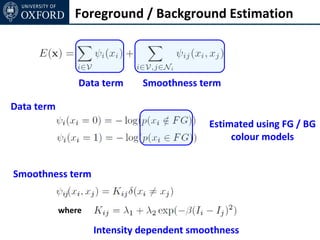
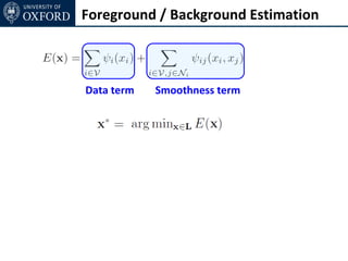
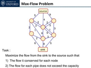
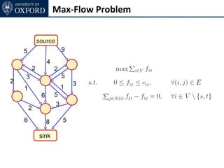
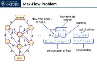
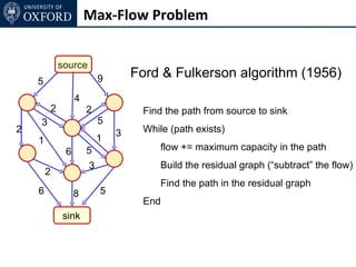
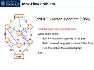
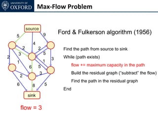
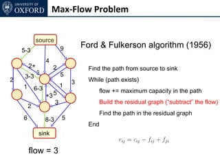
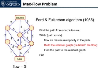
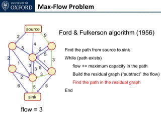
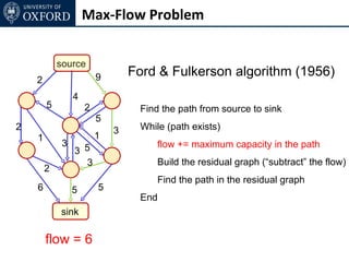
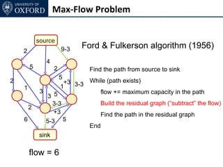
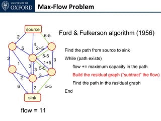
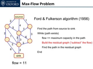
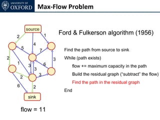
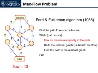
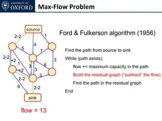
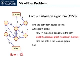
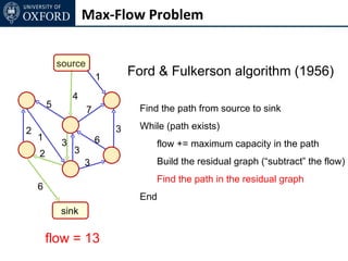
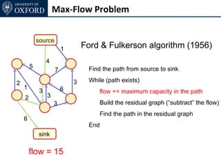
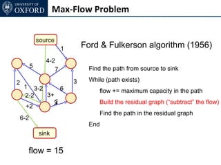
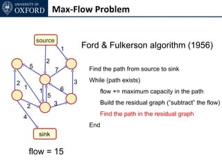
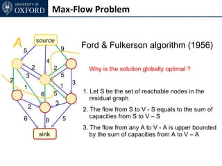
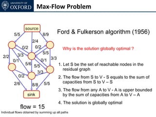
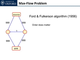
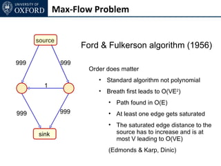
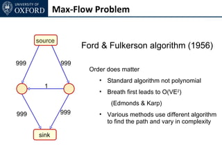
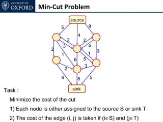
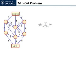
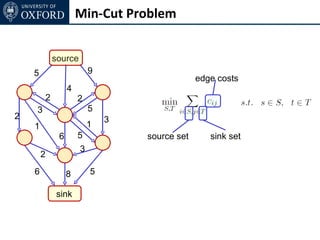
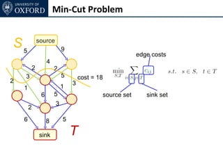
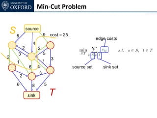
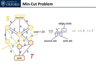
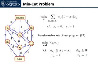
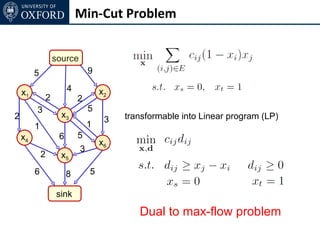
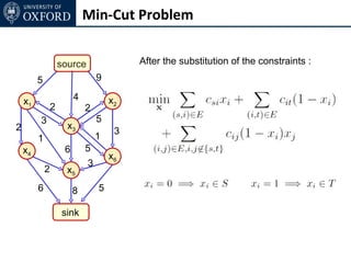
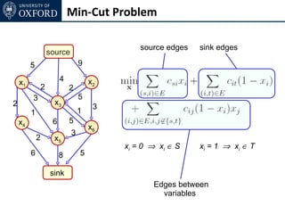
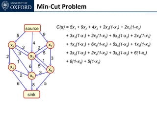
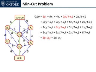
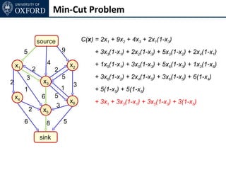
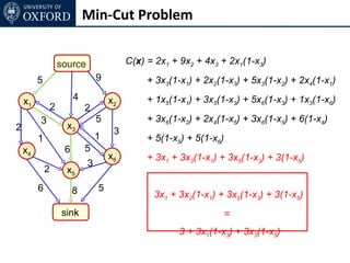
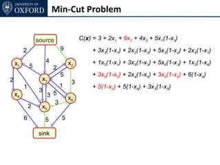
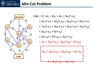
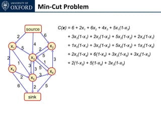
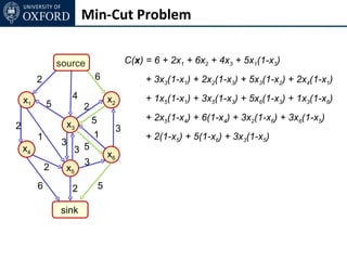
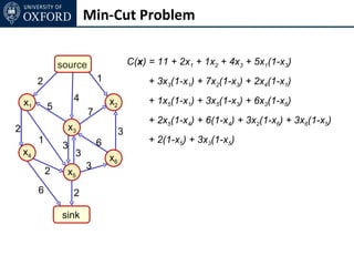
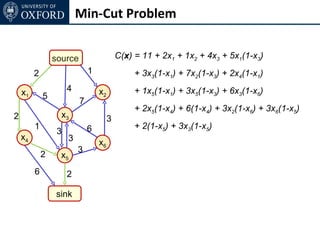
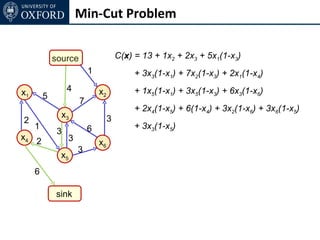
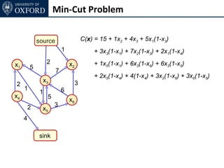
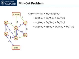
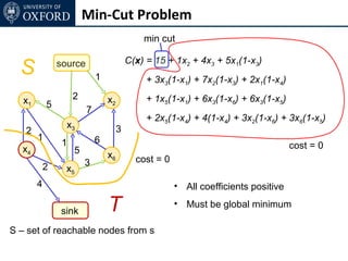
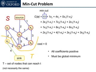
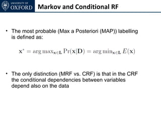
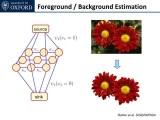
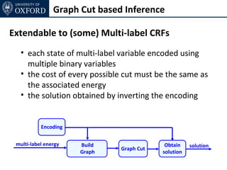
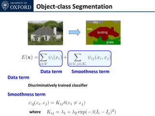
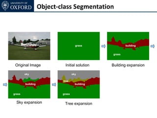
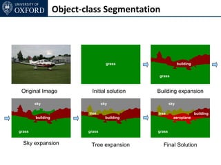
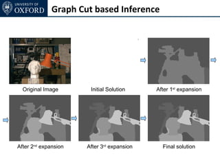
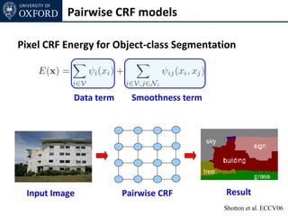
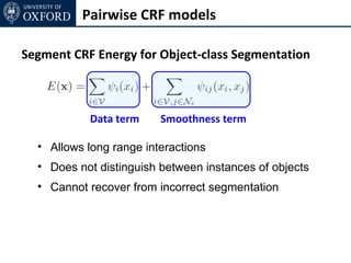
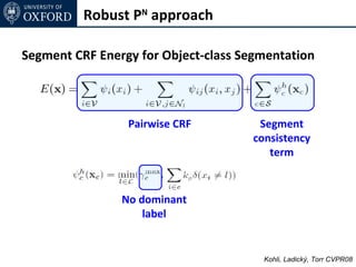
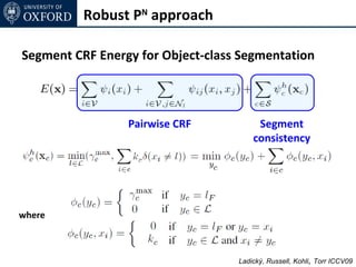
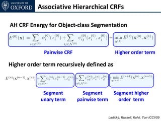
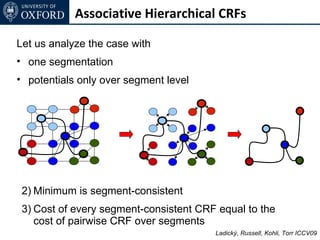
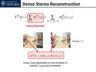
The document discusses graph cut-based optimization techniques for computer vision problems. It describes how image labelling problems can be formulated as energy minimization problems over random fields with complex dependencies between labels. Solving such problems directly is difficult, so the document proposes transforming them into equivalent maximum flow problems on graphs, which can then be solved efficiently using the Ford-Fulkerson algorithm. This allows exploiting graph cuts to optimize random fields for applications like foreground/background segmentation.
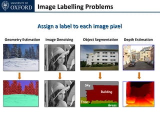


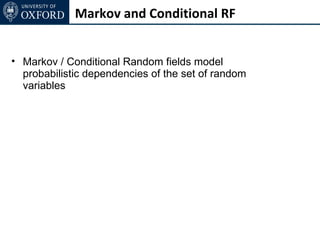


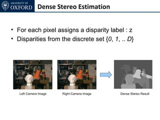
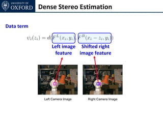
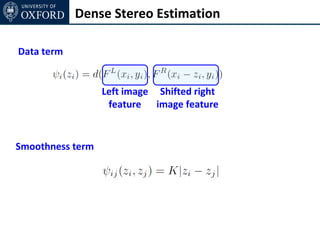
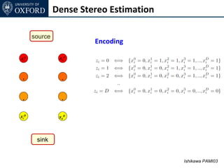

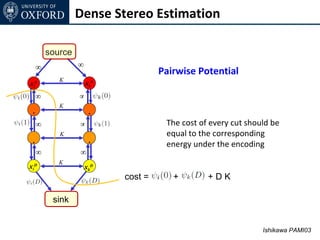
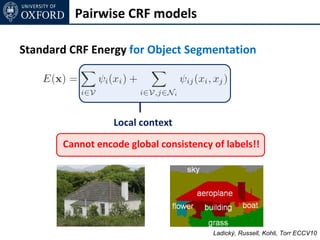
![Dense Stereo Estimation
source
sour
ce ∞ Extendable to any convex cost
∞
xi0 xk0
∞ ∞ xk1 xk2 Convex function
. .
∞ ∞
. .
∞ ∞
xiD xkD See [Ishikawa PAMI03] for more details
sink](https://image.slidesharecdn.com/graphcut-120305013549-phpapp01/85/CVPR2012-Tutorial-Graphcut-based-Optimisation-for-Computer-Vision-117-320.jpg)
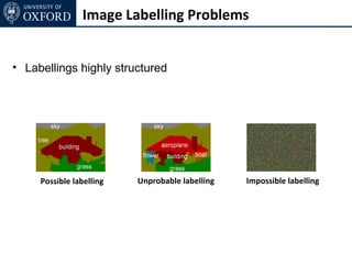
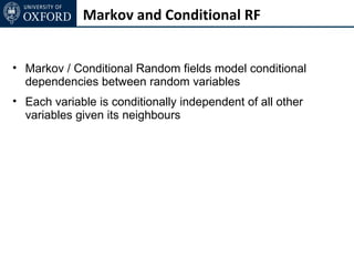
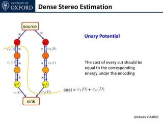
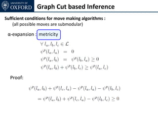
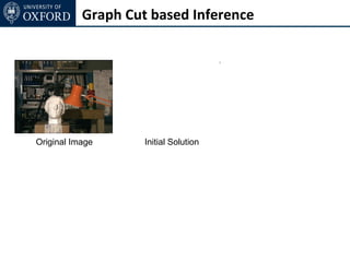
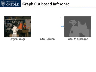
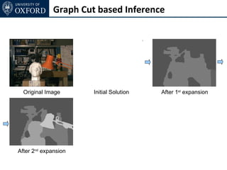
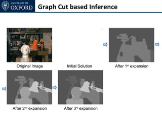
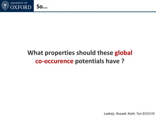
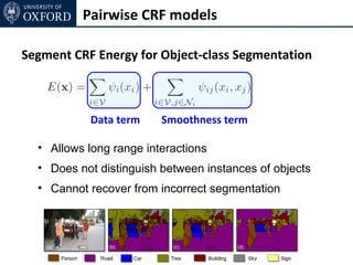
![Graph Cut based Inference
Example : [Boykov et al. 01]
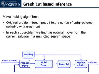
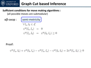
αβ-swap
– each variable taking label α or β can change its label to α or β
– all αβ-moves are iteratively performed till convergence
α-expansion
– each variable either keeps its old label or changes to α
– all α-moves are iteratively performed till convergence
Transformation function :](https://image.slidesharecdn.com/graphcut-120305013549-phpapp01/85/CVPR2012-Tutorial-Graphcut-based-Optimisation-for-Computer-Vision-119-320.jpg)
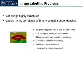
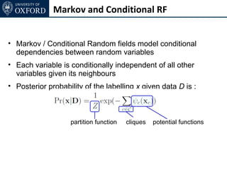
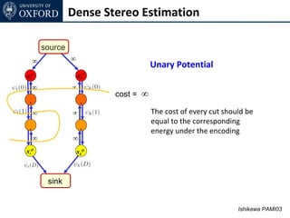
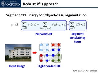
![Graph Cut based Inference
Range-(swap) moves [Veksler 07]
– Each variable in the convex range can change its label to any
other label in the convex range
– all range-moves are iteratively performed till convergence
Range-expansion [Kumar, Veksler & Torr 1]
– Expansion version of range swap moves
– Each varibale can change its label to any label in a convex
range or keep its old label](https://image.slidesharecdn.com/graphcut-120305013549-phpapp01/85/CVPR2012-Tutorial-Graphcut-based-Optimisation-for-Computer-Vision-128-320.jpg)
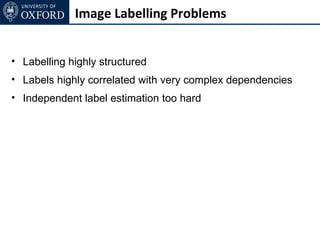
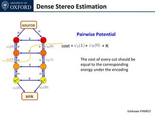
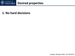
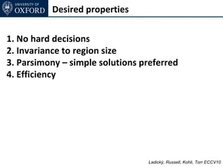
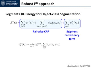
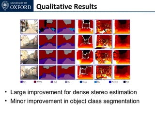
![Encoding Co-occurrence
[Heitz et al. '08]
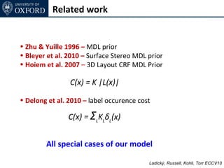
Co-occurrence is a powerful cue [Rabinovich et al. ‘07]
• Thing – Thing
• Stuff - Stuff
• Stuff - Thing
[ Images from Rabinovich et al. 07 ] Ladický, Russell, Kohli, Torr ECCV10](https://image.slidesharecdn.com/graphcut-120305013549-phpapp01/85/CVPR2012-Tutorial-Graphcut-based-Optimisation-for-Computer-Vision-148-320.jpg)
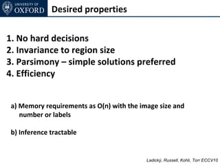
![Encoding Co-occurrence
[Heitz et al. '08]
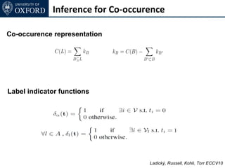
Co-occurrence is a powerful cue [Rabinovich et al. ‘07]
• Thing – Thing
• Stuff - Stuff
• Stuff - Thing
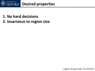
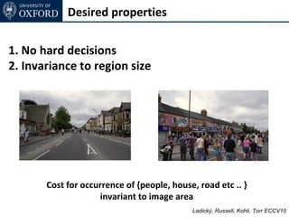
Proposed solutions :
1. Csurka et al. 08 - Hard decision for label estimation
2. Torralba et al. 03 - GIST based unary potential
3. Rabinovich et al. 07 - Full-connected CRF
[ Images from Rabinovich et al. 07 ] Ladický, Russell, Kohli, Torr ECCV10](https://image.slidesharecdn.com/graphcut-120305013549-phpapp01/85/CVPR2012-Tutorial-Graphcut-based-Optimisation-for-Computer-Vision-149-320.jpg)
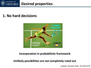
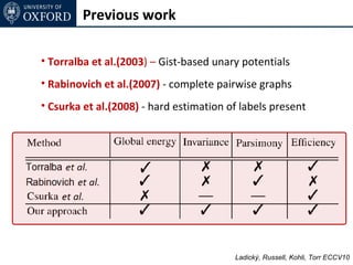
![Inference for Co-occurence
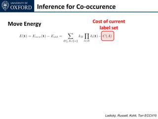
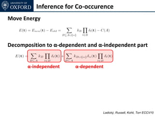
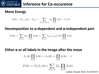
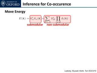
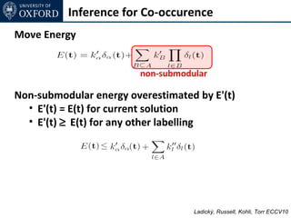
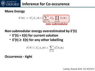
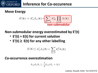
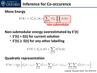
Move Energy
non-submodular
Non-submodular energy overestimated by E'(t)
• E'(t) = E(t) for current solution
• E'(t) ≥ E(t) for any other labelling
General case
[See the paper]
Ladický, Russell, Kohli, Torr ECCV10](https://image.slidesharecdn.com/graphcut-120305013549-phpapp01/85/CVPR2012-Tutorial-Graphcut-based-Optimisation-for-Computer-Vision-170-320.jpg)
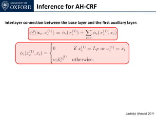
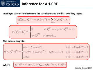
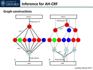
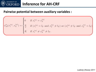
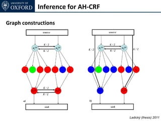
![Inference for AH-CRF
Graph Cut based move making algorithms [Boykov et al. 01]
α-expansion transformation function for base layer
Ladický (thesis) 2011](https://image.slidesharecdn.com/graphcut-120305013549-phpapp01/85/CVPR2012-Tutorial-Graphcut-based-Optimisation-for-Computer-Vision-197-320.jpg)
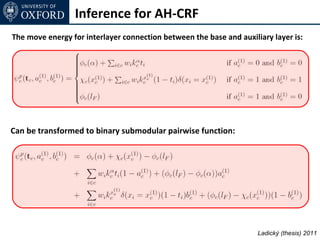
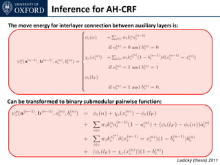
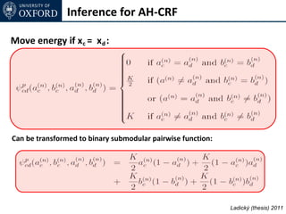
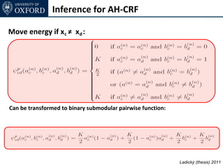
![Inference for AH-CRF
Graph Cut based move making algorithms [Boykov et al. 01]
α-expansion transformation function for base layer
α-expansion transformation function for auxiliary layer
(2 binary variables per node)
Ladický (thesis) 2011](https://image.slidesharecdn.com/graphcut-120305013549-phpapp01/85/CVPR2012-Tutorial-Graphcut-based-Optimisation-for-Computer-Vision-198-320.jpg)


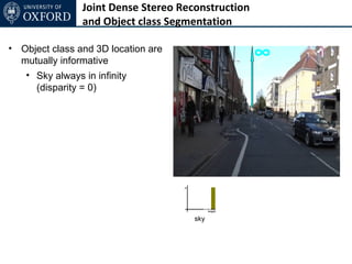
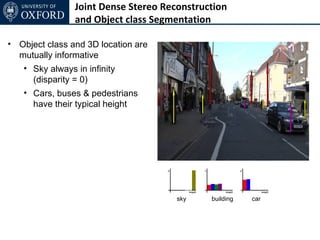
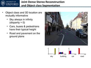

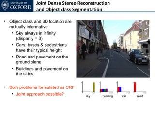
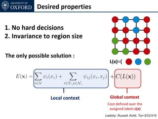
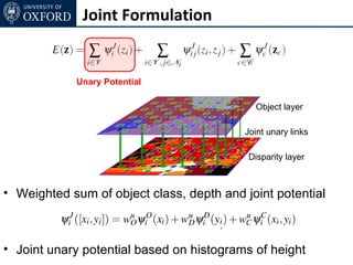
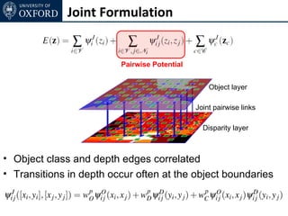
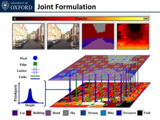
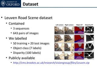
![Joint Formulation
• Each pixels takes label zi = [ xi yi ] ∈ L1 × L2
• Dependency of xi and yi encoded as a unary and pairwise
potential, e.g.
• strong correlation between x = road, y = near ground plane
• strong correlation between x = sky, y = 0
• Correlation of edge in object class and disparity domain](https://image.slidesharecdn.com/graphcut-120305013549-phpapp01/85/CVPR2012-Tutorial-Graphcut-based-Optimisation-for-Computer-Vision-229-320.jpg)
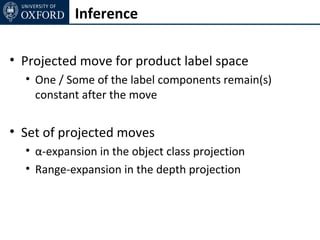
![Inference
• Standard α-expansion
• Each node in each expansion move keeps its old label
or takes a new label [xL1, yL2],
• Possible in case of metric pairwise potentials](https://image.slidesharecdn.com/graphcut-120305013549-phpapp01/85/CVPR2012-Tutorial-Graphcut-based-Optimisation-for-Computer-Vision-233-320.jpg)
![Inference
• Standard α-expansion
• Each node in each expansion move keeps its old label
or takes a new label [xL1, yL2],
• Possible in case of metric pairwise potentials
Too many moves! ( |L1| |L2| )
Impractical !](https://image.slidesharecdn.com/graphcut-120305013549-phpapp01/85/CVPR2012-Tutorial-Graphcut-based-Optimisation-for-Computer-Vision-234-320.jpg)


![Ford_Fulkerson_Algorithm_uptade.ppt[1].pptx](https://cdn.slidesharecdn.com/ss_thumbnails/fordfulkersonalgorithmuptade-250128085250-50c85c74-thumbnail.jpg?width=640&height=640&fit=bounds)


