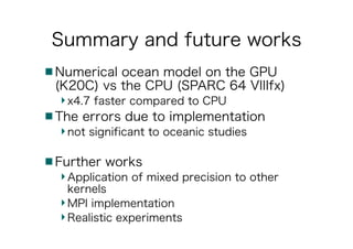
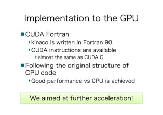
This document discusses the GPU acceleration of a non-hydrostatic ocean model called 'kinaco', highlighting its implementation, optimization strategies, and performance evaluation. The study demonstrates that the GPU-optimized model is approximately 4.7 times faster than the CPU version while maintaining acceptable accuracy for oceanic studies. Future work aims to apply mixed precision techniques to additional kernels and implement MPI for realistic experiments.

1. GPU acceleration of a non-
hydrostatic ocean model with a
multigrid Poisson/Helmholtz
solver
Takateru Yamagishi1, Yoshimasa Matsumura2
1 Research Organization for Information Science and
Technology
2 Institute of Low Temperature Science, Hokkaido University
6th International Workshop on Advances in High-
Performance Computational Earth Sciences: Applications
& Frameworks

2. Table of Contents
Motivation
Numerical ocean model ‘kinaco’
GPU implementation and Optimization
Evaluation and validation
Summary

3. Motivation
Significance of numerical ocean modelling
Global climate, weather, marine resource, etc.
GPU’s high computational performance
Explicit and detail expression, long time
simulation, many experiment cases
Previous studies
Bleichrodt et al. (2012), Milakov et al. (2013),
Werkhoven et al. (2013) Xu, et al. (2015)
They showed high performance, but limited to
experimental studies
We aim at realistic and practical studies

4. Non-hydrostatic numerical
ocean model ‘kinaco’
Formation of Antarctic bottom
water in the southern Weddell Sea
We try to accelerate this model by the GPU

5. Basic equation of dynamics in
kinaco
3D Navier-Stokes equation
Fluid dynamics
Poisson/Helmholtz equation
∆ = , (∆ + )ℎ = 0
Discretization
Stencil access to adjacent 6 grids
Solving systems of equations: Ax=b
Sparse matrix-vector multiplication
Efficient solver to solve Ax=b is required

6. CG method with multigrid
preconditioner (MGCG)
Fast and scalable
iteration method
Matsumura and Hasumi
(2008)
Preconditioner: Multigrid
method
Solve equation on various
resolution grids
multigrid method

7. Implementation to the GPU
CUDA Fortran
kinaco is written in Fortran 90
CUDA instructions are available
almost the same as CUDA C
Following the original structure of
CPU code
Good performance vs CPU is achieved
We aimed at further acceleration!

8. Optimization of the MGCG
solver
The cost of MGCG solver: 21% of total
simulation
Mainly consists of sparse matrix-vector
multiplication
Optimization
1. Memory access
2. Hide latency by thread/Instruction-level
parallelism
3. Mixed precision preconditioner of MGCG

9. Memory access in CPU kernel
DO k=1, n3
DO j=1, n2
DO i=1, n1
out(i,j,k) = a(-3,i,j,k) * x(i, j, k-1) &
+ a(-2,i,j,k) * x(i, j-1,k ) &
+ a(-1,i,j,k) * x(i-1,j, k ) &
+ a( 0,i,j,k) * x(i, j, k ) &
+ a( 1,i,j,k) * x(i+1,j, k ) &
+ a( 2,i,j,k) * x(i, j+1,k ) &
+ a( 3,i,j,k) * x(i, j, k+1)
END DO
END DO
END DO
-3 -2 -1 0 1 2 3
a(-3,i,j,k)～a( 3,i,j,k)
Sparse matrix-vector kernel in the CPU code
matrix coefficient
Location of
matrix coefficient
-3
3
1-1
-2
2
0
CPU thread
load the array
‘a’ in cache line.

10. Memory access in GPU kernel
a(i,j,k,-3)
a(i+1,j,k,-3)
a(i+2,j,k,-3)
thread(id)
thread(id+1)
thread(id+2)
a(-3:3,i,j,k) a(i,j,k,-3:3)
Each GPU thread accesses array “a” with 7 intervals.
a(-3,i,j,k) a(-3,i+1,j,k) a(-3,i+2,j,k)
thread(id) thread(id+1) thread(id+2)
Coalesced access to array “a”

11. Hide latency by thread/Instruction-
level parallelism
Hide latency = do other operations
when waiting for latency
Thread-level parallelism
Switch thread to hide latency
Instruction-level parallelism (Volkov,
2010)
One thread with several independent
operations
Comparison of the two parallelism

12. Case 1: Thread-level parallelism
i = threadidx%x + blockdim%x * (blockidx%x-1)
j = threadidx%y + blockdim%y * (blockidx%y-1)
k = threadidx%z + blockdim%z * (blockidx%z-1)
out(i,j,k) = a(i,j,k,-3) * x(i, j, k-1) &
+ a(i,j,k,-2) * x(i, j-1,k ) &
+ a(i,j,k,-1) * x(i-1,j, k ) &
+ a(i,j,k, 0) * x(i, j, k ) &
+ a(i,j,k, 1) * x(i+1,j, k ) &
+ a(i,j,k, 2) * x(i, j+1,k ) &
+ a(i,j,k, 3) * x(i, j, k+1)
Set many threads as possible (i, j, k)
• 3D (i, j, k) threads are set
• One thread for one grid
Hyde latency by switching many threads

13. Case 2: Instruction-level
parallelism
Independent operations are repeated
i = threadidx%x + blockdim%x * (blockidx%x-1)
j = threadidx%y + blockdim%y * (blockidx%y-1)
DO k=1, n3
out(i,j,k) = a(i,j,k,-3) * x(i, j, k-1) &
+ a(i,j,k,-2) * x(i, j-1,k ) &
+ a(i,j,k,-1) * x(i-1,j, k ) &
+ a(i,j,k, 0) * x(i, j, k ) &
+ a(i,j,k, 1) * x(i+1,j, k ) &
+ a(i,j,k, 2) * x(i, j+1,k ) &
+ a(i,j,k, 3) * x(i, j, k+1)
END DO
Hyde latency with instructions
• 2D (i, j) threads are set
• One thread for one column
(i, j)
Case 2 is
faster

14. Mixed precision for multigrid
preconditioning
Low precision
utilize GPU resources
Preconditioning
Low precision is enough
GPU: Deterioration of
performance with coarse
grids
multigrid method
Number of iterations in CG method
unchanged with/without mixed precision

15. Evaluation, experimental setting
CPU (Fujitsu SPARC64VIIIfx) vs GPU
(NVIDIA K20c)
1 CPU vs 1 GPU
Study of baloclinic instability
Visbeck et al. (1996)
Forcing: Coriolis force, temperature forcing
Structured, Isotropic domain
size: (256, 256, 32)
Time step, simulation time
2min, 5hours (150 steps)
5 days(3600 steps)
256
256
32

16. Performance
CPU GPU_1 GPU_2 GPU_3
Speedup
(GPU_3)
all components 174.2 42.6 39.2 37.3 4.7
Poisson/Helmholtz
solver
36.8 15.8 12.4 10.5 3.5
others 137.4 26.9 26.8 26.8 5.1
Elapsed time[s]: CPU vs GPU
CPU : original CPU code
GPU_1: basic and typical implementation to the GPU
GPU_2: GPU_1 + memory optimization, hyde latency
GPU_3: GPU_2 + mixed precision preconditioning
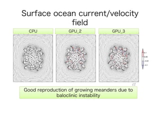
GPU achieved 4.7 times speedup vs CPU
5hours (150 steps)

17. Surface ocean current/velocity
field
GPU_3GPU_2CPU
Good reproduction of growing meanders due to
baloclinic instability

18. Temperature at the cross
section
Good reproduction
of vertical
convection of water
CPU GPU_2
GPU_2

19. Summary and future works
Numerical ocean model on the GPU
(K20C) vs the CPU (SPARC 64 VIIIfx)
x4.7 faster compared to CPU
The errors due to implementation
not significant to oceanic studies
Further works
Application of mixed precision to other
kernels
MPI implementation
Realistic experiments