The document proposes a Discreteness-Aware Approximate Message Passing (DAMP) algorithm for reconstructing discrete-valued vectors from underdetermined linear measurements. DAMP extends existing AMP algorithms to handle discrete variables by incorporating probability distributions of the elements. The algorithm is analyzed using state evolution to derive conditions for perfect reconstruction. A Bayes optimal version of DAMP is also developed by minimizing mean squared error. Simulation results demonstrate improved reconstruction performance compared to conventional methods.

1. Binary Vector Reconstruction
via Discreteness-Aware
Approximate Message Passing
APSIPA ASC 2017 (December 12-15, 2017)
@Kuala Lumpur, Malaysia
Ryo Hayakawa
(Graduate School of Informatics, Kyoto University)
Kazunori Hayashi
(Graduate School of Engineering, Osaka City University)
FP-07 (Special Session)
Large-Scale Stochastic Signal Processing For Wireless Communications

2. Outline
1. Introduction
2. Proposed Algorithm: DAMP
3. Performance Analysis with State Evolution
4. Bayes Optimal DAMP
5. Simulation Result
6. Conclusion

3. Purpose
reconstruction of a discrete-valued vector
from its underdetermined linear measurements
Discrete-Valued Vector Reconstruction
Introduction 1/13
y = Ab 2 RM
Application
✦ overloaded MIMO signal detection [1]
(multiple-input multiple-output)
✦ faster-than-Nyquist signaling [2]
A by NM
reconstruct
ˆb
(M < N)
✦ multiuser detection [1]
✦ overloaded MIMO signal detection [2]
(multiple-input multiple-output)
✦ faster-than-Nyquist signaling [3]
[1] H. Sasahara, K. Hayashi, and M. Nagahara, "Multiuser detection based on MAP estimation with
sum-of-absolute-values relaxation," IEEE Trans. Signal Process., vol.65, no. 21, pp. 5621-5634, Nov. 2017.
[2] R. Hayakawa and K. Hayashi, "Convex optimization based signal detection for massive overloaded MIMO
systems,” IEEE Trans. Wireless Commun., vol. 16, no. 11, pp. 7080-7091, Nov. 2017.
[3] H. Sasahara, K. Hayashi, and M. Nagahara, "Symbol detection for faster-than-Nyquist signaling by
sum-of-absolute-values optimization," IEEE Signal Process. Lett., vol. 23, no. 12, pp. 1853-1857, Dec. 2016.
b 2 {r1, . . . , rL}N

4. Conventional Approach
2/13Introduction
✦ regularization-based method [4]
✦ transform-based method [4]
✦ SOAV optimization [5]
(Sum-of-Absolute-Values)
✦ DAMP algorithm [7]
(Discreteness-Aware Approximate Message Passing)
[4] A. Aïssa-El-Bey, D. Pastor, S. M. A. Sbaï, and Y. Fadlallah, “Sparsity-based recovery of finite alphabet
solutions to underdetermined linear systems,” IEEE Trans. Inf. Theory, vol. 61, no. 4, pp. 2008– 2018, Apr. 2015.
[5] M. Nagahara, “Discrete signal reconstruction by sum of absolute values,” IEEE Signal Process. Lett., vol. 22,
no. 10, pp.1575–1579, Oct. 2015.
[6] D. L. Donoho, A. Maleki, and A. Montanari, “Message-passing algorithms for compressed sensing,”
Proc. Nat. Acad. Sci., vol. 106, no. 45, pp. 18914–18919, Nov. 2009.
[7] R. Hayakawa and K. Hayashi, “Discreteness-aware AMP for reconstruction of symmetrically distributed
discrete variables,” in Proc. IEEE SPAWC 2017, Jul. 2017.
based on convex optimization
❖ low computational complexity
❖ analytical tractability
apply the idea of
AMP (Approximate Message Passing) algorithm [6]

5. Purpose of This Work
Introduction
1 extend the DAMP algorithm for asymmetric distributions
2
3
provide a condition for the perfect reconstruction
derive Bayes optimal DAMP
For binary vector (the simplest case),
Purpose of This Work
[7] R. Hayakawa and K. Hayashi, “Discreteness-aware AMP for reconstruction of symmetrically distributed
discrete variables,” in Proc. IEEE SPAWC 2017, Jul. 2017.
In [7], symmetric distribution of the elements of is assumed.
ex.)
3/13
b 2 {r1, r2}N
not applicable for b 2 {0, 1}N
b
(bj 2 {±1, ±3})(bj 2 {0, ±1})
bj bj bj
ex.)

6. Outline
1. Introduction
2. Proposed Algorithm: DAMP
3. Performance Analysis with State Evolution
4. Bayes Optimal DAMP
5. Simulation Result
6. Conclusion

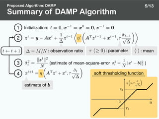
7. Overview of Derivation
Proposed Algorithm: DAMP
✦ unknown vector:
✦ probability:
✦ measurements:
SOAV optimization [5]
Proposed algorithm：DAMP（Discreteness-aware AMP）
apply the idea of
AMP (Approximate Message Passing) algorithm [6]
parameter
b 2 {r1, r2}N
(r1 < r2)
Pr(bj = r1) = p1, Pr(bj = r2) = p2
ˆb = arg min
s2RN
(q1ks r11k1 + q2ks r21k1) subject to y = As
based on the fact that
(, ) hasb r11 b r21
approximately (, ) zero elementsp1N p2N
4/13
[5] M. Nagahara, “Discrete signal reconstruction by sum of absolute values,” IEEE Signal Process. Lett., vol. 22,
no. 10, pp.1575–1579, Oct. 2015.
[6] D. L. Donoho, A. Maleki, and A. Montanari, “Message-passing algorithms for compressed sensing,”
Proc. Nat. Acad. Sci., vol. 106, no. 45, pp. 18914–18919, Nov. 2009.
bjr1 r2
p2
p1

8. (estimate of mean-square-error )
Summary of DAMP Algorithm
5/13Proposed Algorithm: DAMP
: mean
estimate of
: observation ratio
2
Initialization:1
: parameter⌧ ( 0)= M/N
b
soft thresholding function
⌘
✓
u, ⌧ p
◆
xt+1
= ⌘
✓
AT
zt
+ xt
, ⌧
ˆt
p
◆
zt
= y Axt
+
1
zt 1
⌧
⌘0
✓
AT
zt 1
+ xt 1
, ⌧
ˆt 1
p
◆
ˆ2
t =
kzt
k2
N
3
4
t t + 1
t = 0, x 1
= x0
= 0, z 1
= 0
r1
r2

9. Outline
1. Introduction
2. Proposed Algorithm: DAMP
3. Performance Analysis with State Evolution
4. Bayes Optimal DAMP
5. Simulation Result
6. Conclusion

10. [6] D. L. Donoho, A. Maleki, and A. Montanari, “Message-passing algorithms for compressed sensing,”
Proc. Nat. Acad. Sci., vol. 106, no. 45, pp. 18914–18919, Nov. 2009.
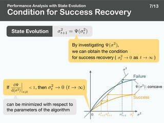
State Evolution
: estimate of at the th iteration
Performance Analysis with State Evolution
: mean-square-error (MSE) of
State Evolution [6]
( 2
) = E
"⇢
⌘
✓
X + p Z, ⌧ p
◆
X
2
#
predict the behavior of MSE
X ⇠ probability distribution of bj
Z ⇠ standard Gaussian distribution
In the large system limit ,
6/13
x
z
ex.)

11. Condition for Success Recovery
Performance Analysis with State Evolution
Success
If , then
Failure
: concave
State Evolution
2
t ! 0 (t ! 1)
2
t+1
can be minimized with respect to
the parameters of the algorithm
By investigating ,( 2
)
we can obtain the condition
for success recovery ( as )t ! 12
t ! 0
7/13

12. 0 0.1 0.2 0.3 0.4 0.5 0.6 0.7 0.8 0.9 1
∆
0
0.1
0.2
0.3
0.4
0.5
0.6
0.7
0.8
0.9
1
p1
Phase Transition
Failure Success
Performance Analysis with State Evolution
observation ratio = M/N
unknown vector:
b 2 {r1, r2}N
Pr(bj = r1) = p1
Pr(bj = r2) = 1 p1
distribution:
8/13
d
d( 2) #0
= 1

13. Outline
1. Introduction
2. Proposed Algorithm: DAMP
3. Performance Analysis with State Evolution
4. Bayes Optimal DAMP
5. Simulation Result
6. Conclusion

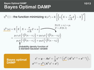
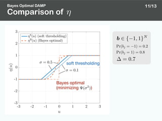
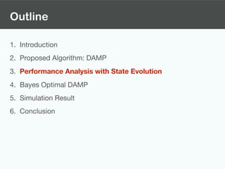
14. Bayes optimal AMP [8]: AMP with minimizing
Bayes Optimal AMP [8]
[8] D. L. Donoho, A. Maleki, and A. Montanari, “The noise-sensitivity phase transition in compressed sensing,”
IEEE Trans. Inf. Theory, vol. 57, no. 10, pp. 6920–6941, Oct. 2011.
( 2
)
Bayes Optimal DAMP
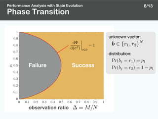
State evolution
AMP algorithm
(in general form)
( 2
) = E
"⇢
⌘
✓
X + p Z
◆
X
2
#
9/13
Any Lipschitz function
can be used
zt
= y Axt
+
1
zt 1
⌦
⌘0
AT
zt 1
+ xt 1
↵
,
xt+1
= ⌘ AT
zt
+ xt
⌘(·)
⌘(·)
smaller is better( 2
)

15. ⌘B
(u) = E

X X + p Z = u
=
p1r1
⇣p
(u r1)
⌘
+ p2r2
⇣p
(u r2)
⌘
p1
⇣p
(u r1)
⌘
+ p2
⇣p
(u r2)
⌘
Bayes Optimal DAMP
Bayes Optimal DAMP
Bayes optimal
DAMP
: the function minimizing
probability density function of
a standard Gaussian variable
Pr(X = r`) = p`
Z ⇠ N(0, 1)
⌘B
(·) ( 2
) = E
"⇢
⌘
✓
X + p Z
◆
X
2
#
zt
= y Axt
+
1
zt 1
D
⌘B0
AT
zt 1
+ xt 1
E
,
xt+1
= ⌘B
AT
zt
+ xt
10/13

16. Comparison of
-3 -2 -1 0 1 2 3
u
-3
-2
-1
0
1
2
3
η(u)
ηS
(u) (soft thresholding)
ηB
(u) (Bayes optimal)
σ = 0.5
σ = 0.1
Bayes optimal
(minimizing )( 2
)
soft thresholding
Bayes Optimal DAMP
⌘
Pr(bj = 1) = 0.2
Pr(bj = 1) = 0.8
b 2 { 1, 1}N
= 0.7
11/13

17. Outline
1. Introduction
2. Proposed Algorithm: DAMP
3. Performance Analysis with State Evolution
4. Bayes Optimal DAMP
5. Simulation Result
6. Conclusion

18. 0 0.1 0.2 0.3 0.4 0.5 0.6 0.7 0.8 0.9 1
∆
0
0.1
0.2
0.3
0.4
0.5
0.6
0.7
0.8
0.9
1
recoveryrate
p1 = 0.3 (soft thresholding)
p1 = 0.6 (soft thresholding)
p1 = 0.9 (soft thresholding)
p1 = 0.3 (Bayes optimal)
p1 = 0.6 (Bayes optimal)
p1 = 0.9 (Bayes optimal)
p1 = 0.6
p1 = 0.9
p1 = 0.3
Definition of success in simulations: at
Success Rate
Simulation Results
Pr(bj = 1) = p1
Pr(bj = 1) = 1 p1
b 2 {0, 1}N
N = 1000
theoretical boundary
successrate
observation ratio = M/N
12/13
rapidly increase around
the theoretical boundary

19. Outline
1. Introduction
2. Proposed Algorithm: DAMP
3. Performance Analysis with State Evolution
4. Bayes Optimal DAMP
5. Simulation Result
6. Conclusion

20. Future Work
Conclusion
✦ application to communication systems
✦ analysis of Bayes optimal DAMP
1
extend the DAMP algorithm
for asymmetric distributions 2
3
provide the condition
for the perfect reconstruction
derive Bayes optimal DAMP
For the reconstruction of binary vector ,b 2 {r1, r2}N
bj
ex.)
0 0.1 0.2 0.3 0.4 0.5 0.6 0.7 0.8 0.9 1
∆
0
0.1
0.2
0.3
0.4
0.5
0.6
0.7
0.8
0.9
1
p1
Failure Success
observation ratio = M/N
13/13