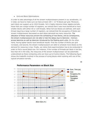
This document summarizes a project report on optimizing fracking simulations for GPU acceleration. The simulations model hydraulic fracturing and consist of three phases. The focus was on the second phase, which calculates interaction factors and stresses between grid cells and takes 80% of the CPU execution time. This phase was implemented on a GPU using techniques like finding parallelism at the cell and grid level, optimizing data transfers, memory access, and using streams to execute cells concurrently. These optimizations led to speedups of up to 56x compared to the CPU implementation.

1. Jose Milet Rodriguez.
Collin Purcell
Dr. Abu-Ghazaleh
CS 217 - CS UCR
12/9/2015
Project Report: Exploring the GPGPU Application Optimization Space. Case of
Study Fracking Simulations.
1.- Introduction
Hydraulic fracturing is a rapidly expanding method of producing fossil fuels. It is the
process of irritating an oil or gas well by pumping a solution of water and proppants under
high pressure from horizontal bores. Computational models of this process help to reduce
the error and waste involved and improve its overall efficiency. Our implementation project
is accelerating a computationally intensive CPU native fracking modeling application to be
used in industry. By accelerating this algorithm, it will be able to be run at higher
resolutions within an industry tolerable execution time. This would translate to a cleaner
more precise frack and less environmental harm.
2.- Problem Description
The simulation has three major phases. We focused on the second phase because it takes
about two days to complete and roughly 80% of the execution time. This phase calculates
the interface stresses and force interaction factors of the irritating solution at its release
stages in the horizontal bores of a fracking well. These metrics are then used to derive the
fluid pressure between each stage in the third phase. Knowing the fluid pressure at these
stages is key to the modeling and control of the fracking process.
Phase two begins by calculating the 3D interactions of a grid of cells in the stages along the
horizontal bores with all the cells previously calculated. To visualize this, the computation
begins by calculating a small subset of interactions. The algorithm then calculates the
interactions of this subset with the cells near it and pushes them into the subset. This
expanding continues until all data is accounted for. It’s important to note that the
interactions calculated are independent from each other and that the input for each
calculation has no reliance on the outputs of others.
To calculate these cell interactions four core functions are used. They comprise of basic
linear algebra calculations, including matrix addition, element by element matrix
multiplication, and matrix transposes. The function list include a distance vector calculator,
a matrix rotator, a interaction factor, and a interface stress calculator. The interaction
factor, distance vector, and matrix rotator functions are called multiple times per element
interaction call. The interaction factor and interface stress functions take 50% and 20% of
the execution time respectively and are very work intensive.
3.- GPGPU Implementation

2. In this section we describe the resources and techniques we use to complete our project.
Since most of the material described here was discussed in class, we don’t describe the
technique itself but rather way we use these them in our implementation.
3.1. Lab Resources Description
All the simulations were executed in a K20c accelerator. The most relevant parameters of
this device include:
Parameter Value Parameter Value
Number Of Cores 2496 Processor Clock 706 MHz
Global Memory 5 GB GDDR5 Memory Clock 2.6 GHz
Memory Bandwidth 208 GB /
Secs
Memory Interfac​ e 320 bits
Stream Processors 13 Max. Thread Block 1024
Peak Single Precision
(GFLOP)
3.52 Tflops Peak Double Precision
(GFLOP)
1.17
Tflops
In addition, all code was compiled with the nVidia nvcc version 4.0 and the GCC compiler
version 4.6. The baselines of our simulations were executed in matlab equipped machine
having an Intel I7 2.3 GHZ processor with 8GB of DDR3 RAM clocked at 1333MHz .
3.2.- Finding Source of Parallelism
The computation of interactions for each cell in the grid can be decomposed into two main
tasks. In the first task we compute the interactions for each cell. In the second task we
iterate over all the cells so as to compute the interactions for all the grid. In order to find
sources of parallelism in the first task, we notice that computing the interactions over a cell
involves the execution of sequential linear algebra operations over a set of two dimensional
matrices sizes N*M. Furthermore all linear algebra operators work at the level of rows. As
result, all linear algebra operations can be computed in parallel since there are no
interactions between adjacent rows. In addition to the two dimensional matrices described
before, computations also are performed along the Z dimension. Usually the computation of
interactions per cell involves the computation of up to 8 N*M planes. Coincidentally, in each
iteration, all linear operators take as input data coming from one single plane. We take
advantage of this independence between rows and planes by executing 3D cuda blocks.
Each grid block works over one row and one plane of the 3D simulation space.

3. In addition to work parallelism at the level of a cell, we observed that interactions between
two cells can be computed in concurrent fashion. For example, if computing the interactions
at the cell level involves the execution of kernels K1, K2, K3, K4 and K5, we observed we
can execute the interactions of two cells by execution two kernels K1, two kernels K2, two
kernels K3 and so on. We can do so as long as we keep independent memory areas for the
inputs and outputs of every kernel. In addition, to further increase the level of parallelism
in the simulation, we notice that 4, 8, and 16 cells can be computed in parallel as well with
minor or no modification of the working code. The only changes that have to be considered
are the changes on indices and the allocation and deallocation of memory areas.
3.3.- GPU Optimizations
The following are the most important GPGPU optimization techniques we used while
working in this project.
● Data Transfer Optimizations
Transferring data between the CPU and the GPU is one of the most expensive operations.
In order to improve the performance of this data transferring process, applications have to
either batch the movement of small chunks of data into large chunks or overlap the
movement of medium size data chunks with the execution of GPU kernels. In addition,
using CUDA memory primitives such as cudaAlloc and cudaFree has its performance
penalty as well. In our implementation, in order to minimize the latency of the data
transferring process, whenever possible, we batch the movement of data between the CPU
and the GPU. Once the data is residing in the GPU we don’t move data data back to the
CPU. Indeed, this is possible because the simulation of every cell uses about 25 MB. In
addition to ​moving the data in batches, we reuse the GPU global memory as to prevent the
use of the GPU primitives for allocating and deallocating memory. When required, we
cleared the global memory, we set areas of global memory to zero, in order to facilitate the
debugging process and to prevent errors. T​his practice was especially true in the initial
versions of our code and it was relaxed in the the final code.
In order to get performance measures about data transfer bandwidth, we designed a
couple of test cases. In the first test case, we measured the CPU-GPU bandwidth when
transferring 4096 matrices size 512*512 in batches both from the CPU to the GPU and
vice-versa. In the second test case we transferred the data in one batch in both directions.
For the first case we were able to achieve host to device bandwidth of 2.00GB/secs and a
device to host bandwidth of 1.28GB/secs. For the second case we were able to achieve a
host to device bandwidth of 3.00GB/secs and a device to host bandwidth of 3.15GB/secs.
From these test cases we concluded that by transferring the data in one single batch we
achieve data movement speed ups of 1.5X and 2.46X respectively. In brief, based in these
measures, we decided to move our simulation data from the CPU to the GPU in one batch.
Yet there are few matrices that have to be moved from the CPU to the CPU as the
simulation progress.

4. ● Grid and Block Optimizations
In order to take advantage of all the stream multiprocessors present in our accelerator, 13
in total, we have to make sure we have at least 104 = 13 *8 blocks per grid. Moreover,
each block can support up to 1024 threads. Yet in highly intensive linear algebra kernels,
these that use a large number of registers, we noticed that it was more beneficial to have
smaller blocks with either 64 or 128 threads. When full size blocks are defined, with each
thread requiring a large number of registers, we noticed that the occupancy of blocks per
stream multiprocessor decreased as each block demands too many resources. ​The
allocation of these resources prevent the scheduling of new blocks, and as consequence,
the stream multiprocessors are not able to hide the delays due to latencies - memory
access latencies as well as latencies introduced by the floating point units.​ On the other
hand, having lighter blocks have beneficial results. First the number of blocks per grid
increases, and second, the stream multiprocessors are able to schedule more blocks as the
demand for resources is low. Finally, we notice that experimentation has to be conducted in
order to find a sound block size. For instance, if the number of threads per block is too low,
less than 64 in the k20c, the resources of the stream multiprocessor can be potentially
underutilized as these computing units can have up to 8 active blocks. The following figure
shows the tradeoffs involved in the process of sizing blocks when working with one of the
typical simulation kernels.

5. In the x-axis the block size is displayed. In the y-axis parameters such as the execution
time, in milliseconds, the multiprocessor average occupancy, in percentage, and the
combined read and write throughput, in GB/s, are shown. In the figure we notice that as
the block size increases from 32 to 128 threads per block the kernel execution time
increases. The kernel occupancy and the kernel memory throughput explain the causes of
these increases in execution time. As the kernel size increases the memory throughput
decreases and the average multiprocessor occupancy increases. Even though having large
occupancies is in most of the cases beneficial at the time of decreasing the kernel latencies,
in the kernel under analysis this is not the case. As shown in the figure, large occupancies
decreases the memory throughput. Because memory access are very expensive, hundreds
core cycles or so, in this particular kernel it is better to have low multiprocessor occupancy.
As illustrated, improving the performance of kernels is a complex task. Some kernels are
very sensible to changes of the global memory throughput while other kernels are more
sensible to changes in multiprocessor occupancy or floating point throughput.
● Global Memory Optimizations.
Making sure all global memory reads and writes are coalesced is an important optimization
te​chnique when implementing GPGPU based applications. In order to take advantage of this
technique we analyzed the way kernels access global memory in our code. After inspecting
our implementation, we realized that kernel’s threads access data in both row and column
fashion. In order to speed up our code, we decided to dynamically change the layout of the
data as to make sure all global memory reads are executed in a coalesced fashion. For
example, if the threads in kernel K2 read the data in row fashion, i.e. a single K2 thread
reads all the elements of a row, previous to the execution of K2 the data layout was
changed from row major to column major. In the new data layout, the column major,
threads T1 and T2 in K2 can take advantage of coalesced reads as they access elements of
contiguous columns. Yet in the case of global me​mory writes, coalesced writes were not
always possible. For instance, if sequential kernel K4 requires the data in row major,
sequential kernel K3 makes sure it outputs the data in a row major layout at the expenses
of lowering the throughput of writes to global memory writes. In addition, we considered
the use of specific kernels to transpose the data but we did not implement this option as
launching new kernels has large overhead. When optimizing the kernels for memory
throughput, we faced cases where even changing parameters as block size or amount of
work per thread, thread coarsening, did not help. The following figure illustrate such case.

6. In this figure, we changed the block size from 32 to 256 threads and observed the behavior
of other parameters namely multiprocessor average occupancy and global memory
throughput. First we notice that as the number of threads per block increases, the average
execution time and the global memory throughput remains constant. Moreover the
multiprocessor occupancy increases rapidly when the block size goes from 128 to 256
otherwise it remains constant. To optimize the latency of this kernel we tried to change
parameters such as block size, amount of work per thread, usage of cache memory without
success. After close inspection of the code, we hypothesized that updates to global memory
where hurting the performance. In order to prevent updates, we decided to write the kernel
output values in new areas of memory and execute the updates later in another kernel.
After this change we implemented we were able to double the global memory throughput
and increase the occupancy for about 50%. As result, the execution time of the kernel
decreased by about 4 milliseconds: a gain of 15% in the execution time and and speed up
of about 5X in the overall simulation time. All in all, in the task of decreasing the latency of
kernels often we hit a local minima as we do with other optimization tasks. Getting out of
these local minima is not always an easy task and often it requires the redesign of the
kernel.
● Constant Memory Optimizations
Our k20c GPGPU accelerator is equipped with 64KB of constant memory. While GPU kernels
can only read the data in constant memory, CPU applications are able to read and write it.
Since constant memory is equipped with a local memory cache, we wanted to further
optimize our application by making user of this resource. To do so, we noticed that a set of

7. small vectors sizes 1*4 are used during the computation of interactions per cell.
Particularly, the values of these matrices are defined previously to computing cell
interactions and these vectors do not change during the cell simulation. In this regard, we
modified our code such that the CPU writes these vectors in the device constant memory
and the GPU reads these values when required.
● Streams
After a close inspection of the code, we realized that it was possible to execute the
simulation of two or more cells in a concurrent fashion. For example if the simulation of
each cell requires kernels K1,K2, K3 and K4 we noticed it was possible to interleave the
execution of these kernels for multiple cells. In post Fermi GPU architectures, interleaving
cell executions allow them to share the GPU’s execution space and increase throughput at
the cell level. After optimizing the cell latencies in a single stream with the above outlined
techniques, increasing the cell throughput was our next goal. To achieve this we targeted
the use of streams. Our implementation aggregated all data movements and kernel
executions related to the simulation of a cell into a single stream. This made every stream
independent and self contained. Below is a visualization of the kernel execution overlapping
one of our kernels achieved using 16 streams.
Using Nvidia’s visual profiler, we took this snapshot of our kernel execution concurrency for
the execution of one chunk of 16 streams. Note that there are no gaps between kernel calls
between streams. This keeps the GPU busy at all times during this kernel's execution
across the streams. Also notice that there are up to 5 streams executing concurrently. This
translates to more throughput at the cell level, and higher GPU occupancy and memory
throughput since our kernels do not individually saturate all its resources. At the simulation
level the increase in cell throughput, higher utilization of GPU resources, and reduction of
the time gaps between kernel calls translated to drastic runtime speed ups shown in the
graph below.

8. This graph plots the simulation time as we increase the number of streams from 1 to 16.
Using 1 stream had an 18x speed up, 2 streams a 26.6x, 4 streams a 39.0x, 8 streams a
48.5x, and 16 streams a 56x. Notice the diminishing returns from adding streams as GPU
resources saturate. For example, the simulation time decreased 31.04% when going from 1
stream to 2, but only 12.6% when going from 8 to 16 despite adding 8x more streams.
This means that each of the 8 streams added to go from 8 streams to 16 streams only
decreased the execution time 1.58%. Never-the-less, streams proved to be an invaluable
optimization for our simulation.
● Thread Coarsening
A key metric for the kernel execution overlapping shown above is the kernel’s execution
time. By inspecting the profiles of our kernel execution and overlapping we noticed that
kernels with execution times 30 microseconds or less are not able to take advantage of the
space sharing execution capabilities of the GPU. Furthermore, as stated by the GPU
documentation, launching a kernel has on overhead of about 5 microseconds. Our goals
were two. We wanted to lengthen these kernel’s execution times to increase the
probabilities of concurrent execution in short latency kernels as well as increase the ratio of
work to kernel launch overhead. To do this we decided to increase these kernel’s amount of
work per thread in a process called thread coarsening. Below are the results of our
optimization changes.

9. On the left is a snapshot of a kernel in nvidia’s visual profiler without any thread coarsening
and an execution time of 11us. Here, there are gaps between stream’s kernel calls without
any execution overlapping. On the right is that same kernel with thread coarsening. Each
thread now does 5x the amount of work, lengthening the kernel’s execution time to 40us.
Now that the kernel’s execution times are over 30us, the streams have no space between
their kernel calls and have a maximum of 3 kernels overlapping their execution. These
snapshots of the visual profiler show how on a cell execution level thread coarsening
changes the execution and scheduling of our kernels. The graph below shows how these
changes affected the runtime of our simulation.

10. This graph shows the relationship of the simulation time of 500 cells to the amount of
thread coarsening we used. The numbers in the x-axis represent the units of work we
assigned to the threads in kernels K1, K2, K3 and K4. For instance the label 1,1,1,1
indicates that each thread in kernels K1, K2, K3, and K4 executes one unit of work.
Likewise the label 2,5,5,5 indicates that a thread in kernel K1 executes two units of work
and threads in kernel K2, K3 and K4 execute five units of work. Here units of work refers to
basic operations such as vector addition, for example. Through experimentation we found
that the ideal amount of work coarsening was 2,5,5,5. At the simulation level, we were able
to decrease our runtime by 16.25% using thread coarsening.
4.- Results
Using the above detailed techniques, we were able to achieve a 50x increase in execution
time over a matlab implementation running on an i7 processor. The initial 10x of this was
due to optimizing memory transactions, optimizing memory allocation, and layering the
data to add parallelism. The next 10x was from kernel and memory accessing
optimizations. In this stage we spent hours resizing and recombining our kernels to find the
optimal balance of GPU occupancy, memory throughput, and resource management. The
next 30x execution speed up came from streams. The last 5x execution speed up came
from thread coarsening and grid size optimizations. Using the CUDA toolkit profiling metrics
we found that the average memory throughput for our functions was 32.25GB/s, and our
average GPU occupancy was 34.65% per stream. In practice these numbers are higher
because more than one kernel is executing at once on average.
To do this we focused on leveraging the GPU’s enormous compute power and wide memory
bandwidth to exploit the intrinsic parallelism in the simulation at hand . This was not a
straightforward processes, however. We spent tens of hours in the beginning exploring
single stream optimizations, often running into walls and experiencing drawbacks. It was in
this phase we explored techniques for resource optimizations, mainly memory bandwidth
and kernel execution. In addition, this phase allowed us to discover the hidden sources of
parallelism within our application. Without previous work on our code for direction and very
little background information on the application, all of our work was based in good insight
and experimentation based in test cases. We worked very carefully and methodically
through these single stream optimizations, and did not implement multiple streams until
we were confident that the latencies in the single stream implementations were minimal.
When we did instantiate multiple streams we made the transition from latency oriented
design to throughput oriented design. This meant repurposing our latency oriented fast
executing kernels to longer more throughput oriented ones with thread coarsening. It also
meant cutting back on the resources required per kernel to allow for space sharing between
streams and more kernel throughput. From memory optimizations, latency vs throughput
oriented optimizations, and an eye for structural parallelism, this project has given us a
tremendous breath of new insights that we can bring to our future projects.

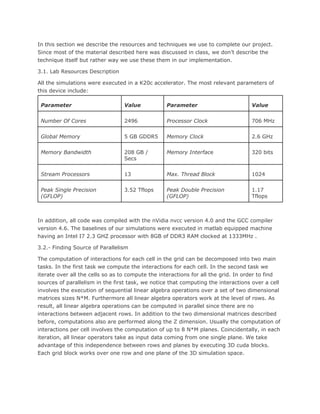
11. While exploring the optimization space of the application at hand we have make heavily use
of performance metrics including global memory throughput per kernel, floating point and
integer operations executed per kernel, instructions executed per cycle per kernel, cache
utilization per kernel, and achieved occupancy. Among these parameters, improving the
achieved occupancy per kernel has been our guiding metric. Occupancy per stream
multiprocessor can be improved by either decreasing the kernel latencies or by increasing
the throughput of the number of kernels we execute in the unit of time. In our initial
implementation our goal was to decrease the time execution latencies of the simulations
per cell. To pursue this goal we optimized parameters such as data traffic via the PCI bus,
number and shape of kernels, data layouts, usage of constant memory, degree of
parallelism among others. Next, because of the high number of cells, we pursued to
increase the cell throughput, the number of cells simulated in the unit of time. Our
guiding idea was to increase GPU occupancy at the expenses of increasing the cell
latencies, the time it takes to simulate the interactions over one cell. Here our goal was to
simulate multiple cell in parallel. To achieve this goal we relaxed the latencies per cell,
using techniques such as thread coarsening, and create multiple cuda streams. Eeach
stream been responsible for the simulation of a cell. This approach boosted the
performance of our application as we were able to achieve a speedup of up to 50X. Yet
increasing cell throughput or decreasing the cell latencies are only possible by shaping the
the size of the blocks and the grids, shaping memory throughputs, increasing or
decreasing the number of floating point or integer operations and the alike. To the end,
exploring the optimization space of GPGPU applications is a complex task due in principle to
the drastic changes, the nonlinearities, present when one variable or more variables, for
instance the usage of registers per thread for instance, are altered.
5.- Related Works
The fracking algorithm we implemented is private property, confidential and unique.
However the basic structure is similar to a stencil all pairs n-body calculation which has
been heavily documented. Both our algorithm and an all pairs n-body algorithm share the
same element by element force calculations. Due the similar structures we found parallels
between our fracking implementation and the all pairs n-body implementations. For
example, [1] proposes that in dislocation dynamics n-body simulations shared memory is
not optimal when data overflows into register memory. We did not use shared memory for
this reason and due to little reuse of memory in our algorithm. [1] also removed
intermediate variables from global memory, choosing to calculate them on the fly and keep
them in register memory. We also implemented this strategy. [2] contrasts with [1],
suggesting to use tiles and shared memory. We decided to use [1]’s strategy because our
algorithm has very little memory reuse within our kernels. We did however implement
constant memory as was done in [2]. Many all pairs n-body calculations use one thread per
cell to calculate thousands in parallel, like [3] suggests. Each cell in our implementation
requires too many resources to launch enough single cell threads to fill the GPU. For this
reason we could not use the typical all pairs n-body 1 thread per cell structure. Another

12. strategy we used that is used in [4]’s n-body all pairs calculation is the reduction of
CPU-GPU memory traffic. Both our implementation and [4]’s move as much of the memory
to the GPU in the beginning of the algorithm as possible, and leave it there until all work
requiring that data is finished. Finally, we implemented thread coarsening which as shown
by [5] has minimal execution boost for n-body calculations. However, when we
implemented thread coarsening we achieved a 1.16X speedup due to differences in the
natures of our kernels and typical n-body kernels.
References.-
[1] Ferroni, Francesco, Edmund Tarleton, and Steven Fitzgerald. "GPU Accelerated
Dislocation Dynamics." GPU Accelerated Dislocation Dynamics. Journal of Computational
Physics, 1 Sept. 2014. Web. 10 Dec. 2015.
[2] Playne, D.P., M.G.B. Johnson, and K.A. Hawick. "Benchmarking GPU Devices with
N-Body Simulations." (n.d.): n. pag. Benchmarking GPU Devices with N-Body Simulations.
Massey University. Web. 10 Dec. 2015.
[3] Nyland, Lars, Mark Harris, and Jan Prins. "GPU Gems 3." - Chapter 31. Fast N-Body
Simulation with CUDA. NVIDIA Corporation, n.d. Web. 10 Dec. 2015.
[4] Burtscher, Martin, and Keshav Pingali. "An Efficient CUDA Implementation of the
Tree-Based Barnes Hut N-Body Algorithm." An Efficient CUDA Implementation of the
Tree-Based Barnes Hut N-Body (n.d.): n. pag.Parallel Scientific Computing. Southern
Methodist University, 2011. Web. 10 Dec. 2015.
[5] Magni, Alberto, Christophe Dubach, and Michael O'Boyle. A Large-Scale
Cross-Architecture Evaluation of Thread-Coarsening. IEEE Xplore. Univ. of Edinburgh,
Edinburgh, UK, n.d. Web. 10 Dec. 2015.