Mapping spatial variability of soil physical properties for site-specific management

International Research Journal of Engineering and Technology (IRJET) e-ISSN: 2395 -0056
Volume: 03 Issue: 02 | Feb-2016 www.irjet.net p-ISSN: 2395-0072
© 2016, IRJET | Impact Factor value: 4.45 | ISO 9001:2008 Certified Journal | Page 149
Mapping spatial variability of soil physical properties for site-specific
management
Henry Oppong Tuffour1,*, Awudu Abubakari1, Janvier Bigabwa Bashagaluke1,2, Ebenezer
Djaney Djagbletey1,3
1Department of Crop and Soil Sciences, Kwame Nkrumah University of Science and Technology, Kumasi, Ghana
2Department of Soil Science, Faculty of Agriculture, Catholic University of Bukavu, DR Congo
3Ghana Forestry Commission, Cape Coast
---------------------------------------------------------------------***---------------------------------------------------------------------
Abstract - Description of the spatial patterns of soil
properties at the field or watershed scale is very importantfor
site-specific soil and crop management, and environmental
modelling. The study was conducted to determine the spatial
distribution patterns of soil physical properties in an
agricultural field in the surface (0-20 cm) and subsurface(20-
40 cm) layers. Descriptive statistics and geostatistics were
used to describe the amount and form of variability and
spatial distribution patterns of the soil physical properties in
the field using GraphPad Prism version 6.0 and GS+ 9.0,
respectively. The descriptive statistics revealed that the soil
properties exhibited weak to higher variations in both layers
cross the field, with aggregate stability beingthemostreliable
soil physical property in the field. The spatial distribution
model, spatial dependence levelsandspatialdistributionmaps
showed remarkable variations in both layers across the field.
The significance of semivariogram modelling for the
subsequent interpolation was proven to beaneffectivetool for
delineation of management zones for site-specific soil
management.
Key Words: Autocorrelation, kriging, semivariogram, site-
specific soil management, spatial dependence
1. INTRODUCTION
Spatial variability ofsoil physical propertieswithinoramong
agricultural fields is inherent in nature due to both geologic
and pedologic factors of soil formation. However,
management practices such as tillage, irrigation, and
fertilizer application may also induce variability within the
field and may further interact with each other across
different spatial and temporal scales, and are further
modified locally by erosion and deposition processes [1].
Spatial properties of field soils, thus, vary in a complex
manner, especially in arid and semi-arid environments
where this phenomenonaffectsthequalityandproductionof
crops, hydrologic responses and transport of herbicides to
surface and/or groundwater. [2, 3]. Traditionally,
researchers have attempted to remove spatial variability by
blocking and/or statistical averaging procedures. However,
these attempts have often resulted in the failure to
understand the spatial interdependence of the soil
properties. An appropriate understanding of the spatial
variation of soil properties and the relationships between
them is needed to scale up measured soil properties, and
model soil processes for precision farming/forestry and
environmental modelling. The study was, therefore
conducted to analyze the extent of spatial variability in
selected soil physical properties.
2. MATERIALS AND METHODS
2.1. Site location and characteristics
The study was conducted at the Plantations Section of the
Department of Crop and Soil Sciences, of the Kwame
Nkrumah University of Science and Technology, Kumasi,
Ghana. The experimental field was locatedinanuprootedoil
palm (Elaies guineensis) field, where spatial variability was
predictable due to the variable biological activity and the
presence of dead root channels and burrows of soil animals
[4]. The area is within the semi-deciduous forest zone of
Ghana. It is subjected to two growing seasons (a major and a
minor season) with a bimodal rainfall pattern. The major
season starts in May and is interrupted by a dry period in
August. The minor season starts from September to
November. Annual rainfall is about 1375 mm. Annual
temperature ranges from 25 – 35°C. The dominant soil is the
Kumasi series described as Plinthi Ferric Acrisol [5]orTypic
Plinthustult [6].
2. Design of sampling grid and soil sampling
A total field of 75 x 40 m was gridded with 10 x 5 m intervals
in the north to south and east to west directions, and soil
samples were collected at 80 intersection points, since
geostatistical analyses requires at least 50 – 100 measuring
grid points [4,7]. The sampling grid size was chosen because
as a “rule of thumb”, the estimation of semivariograms is
considered reliable for lags not exceeding 20% of the total
transect length [8]. The sampling points were established
and maintained using a Global Positioning System (GPS)
device, and systematically located at the nodes of a
rectangular shaped object superimposed on the field and
systematic grid sampling was employed, since there was
little prior knowledge of the within-field variability,andalso
offered the advantage of applying simple techniques to map
attributes within the field. Regarding the soil as an
anisotropic medium, varying in both vertical and horizontal
dimensions, the fundamental feature of horizonation was
considered and soil samples were collected from the 0 – 20
cm and 20 – 40 cm depths.

2.3. Soil sampling and analyses
Cylindrical core samplers of 8.1 cm diameter and 20 cm
length were used for the collection of soil samples. The
collected samples were used for the analyses of particle size
distribution using the hydrometer method [9], volumetric
moisture content [10], bulk density and total porosity [11],
and aggregate stability [12].
2.4. Data analyses
Measured variables in the data set were analyzed in two
distinct stages. First, the descriptive statistics including the
minimum, maximum, mean, coefficient of variation (CV),
skewness and kurtosis were estimated for each property at
each depth using GraphPad Prism version 6.0.
Characterization of CV was conducted as described by
Tuffour et al. [4] and Wilding [13]. The symmetry and
peakedness of the data distribution basedonthecoefficients
of skewness and kurtosis were used to determine the order
of data distribution in the field. However, since it was
expected that small variations could arise and produce a
chance fluctuation of skewness and kurtosis measures from
zero (Normal distribution), each variable was validated to
determine the type of distribution from which the samples
were taken using the D’Agostino-Pearson “OmnibusK2”test
[4, 14].
Geostatistical calculations and interpolations were used to
describe the spatial dependence of each soil property using
GS+ 9.0 software. Regarding the fact that normality of
distribution is not a pre-requisiteofgeostatistical processing
the original data set was processed without any
transformation [4, 15]. Spatial variability was evaluated
using the semivariogram for both isotropical and
anisotropical orientations. The anisotropic evaluationswere
performed in four different directions (0°, 45°, 90° and 135°)
with a tolerance of 22.5° to determine whether
semivariogram functions depended on samplingorientation
and direction (i.e., they were anisotropic) or not (i.e., they
were isotropic), and the commonly used models were fitted
for each soil property [4]. The best fit model was chosen
using the Least Squares method and the spatial dependence
(SD) was defined using the nugget/sill ratio [4, 16]. Surface
maps of the soil properties were prepared using
semivariogram parameters through ordinary Kriging and
prediction performance was assessed by cross-validation
[4].
3. RESULTS AND DISCUSSIONS
3.1. Descriptive statistics
The spot-to-spot variations in the soil physical properties as
observed from the measured descriptive statistical values
are presented in Table 1. The results showed significant
differences between the mean values at both sampling
depths across the field. These variationscouldbeascribedto
a combination of factors including experimental errors, and
temporal and spatial variations.
3.1.1. Variation in particle size distribution
The top layer showed different textural classes of loamy
sand, sandy loam and sandy clay loam. Except for two spots
with sand, and sandy clay texture each, soils in the
subsurface were dominantly sandy loam and loamy sand
textured. The coefficients of variation for sand content in
both layers were classified as low, whereas those of silt and
clay were classified as very high, with the sub surface layer
showing higher variability than the upper layer. Among the
primary soil particles, the mean sand and silt contents were
slightly lower in the subsurface layer than in the surface
layer, whereas the mean clay content was higher in the
subsurface layer than in thesurfacelayer.ThehighCVvalues
of silt and clay could have resulted from the previous land
use system and soil management strategies in the field.
Although studies by Santra et al. [17] showed that soil
mixing due to tillage operations can result in little variation
of particle size distribution in the surface layer than the
subsurface layer, the modified minimum tillage method
employed in the land preparation process in this study
yielded similar results, except for clay content. The low
variability of particle size fractions at the surface layer as
compared to the subsurface layer could, thus, be attributed
to the susceptibility of the soil aggregates to erosion and
deposition of soil particles from one spot to another in the
field. This is because these processes tend to distribute the
soil particles, somehow, uniformly in the field. Additionally,
the eluviation-illuviation processes due to downward
movement of water through thesoil mayhaveresultedin the
deposition of fine-grained particles (especially clay) within
the underlying layers beneath the soil surface. The
differences in the influence of parent materials (i.e.
resistance or susceptibility to weathering) may also have
affected the distribution of soil particles in the field.
Silt and clay fractions gave positive and highest kurtosis in
the surface layer and subsurface layers, respectively. The
kurtosis value for sand in the surface layer, although
positive, showed a normal (mesokurtic) distribution, not
only because it was closer to zero, but also established from
the K2 test. On the other hand, the kurtosis values for the
different soil fractions in subsurface layer were too tall or
slender than a normal distribution. The results also showed
positive skewness for clay and silt contents, and negative
skewness for sand content in both layers. Similarly, even
though the coefficient of skewness for sand in the surface
layer extended toward the left, showing a shift from normal
distribution, the K2 test revealed itwasnormallydistributed
across the field. This indicates that the variation of sand
content in the surface layer as revealed by the coefficient of
variability could be due to chance.
3.1.2. Variation in soil structure indicators
Soil structure in the experimental field was described in
terms of bulk density, total porosity and aggregate stability.

From the results, average bulk density and total porosity
were highly variable in the surface layer than thesubsurface
layer, however, the variation in bothlayerswerecategorized
as weak as revealed by the coefficients of variability [4,13].
Similarly, values of aggregate stability in both layers,
although very low, were found to be weakly variable,
indicating an almosthomogeneousaggregatestabilityacross
the field. This could be accredited to the high susceptibility
of the soil aggregates to erosion and depositional events
occurring at the soil surface, causing an almost evenly
distribution of the soil aggregates at the soil surface. On the
other hand, the differences in organic carbon [4] and
moisture contents in both layers could be accountable for
the unequal distribution of aggregate stability with depth.
Thus, aggregate stability was described as the most reliable
soil property in the field, implying that any single valuefrom
any spot in the field for a particular layer could be used to
represent the whole field for that particular layer. The low
aggregate stability observed within both layers could be
attributed to the previous tillage operations (ploughing and
harrowing), which caused significant disturbance to the
surface and subsurface soil structure, organic matter and
clay contents resulting in considerable amounts of
compaction as evidenced by the high bulk density and low
total porosity. This further resulted in the destruction ofsoil
aggregates [18]. The relatively high aggregate stability
observed in the surface layer thanthesubsurfacelayercould
have resulted from the accumulation of organic residues
(high organic carbon content) on the soil surface [4].
With regards to the frequency distribution, the kurtosis
values for aggregate stability in both layers were negative
and platykurtic (i.e., flat). However, the coefficients of
skewness were zero, signifying that aggregate stability was
normally distributed across the field in both layers. Except
for one outlier, which caused a tall peaked distribution, the
distribution of aggregate stability of the surface layer was
almost uniform and flat across the field as evidenced by the
coefficient of variation (0.16%), which was the weakest for
the entire data set in the study. The K2 test values further
showed that aggregate stability was normally distributed
within the field in both the surface and subsurface layers.
For bulk density and total porosity in the surface layer, the
coefficients of kurtosis were positive and close to zero,
which described a leptokurtic distribution. Moreover, the
coefficients of skewness for the properties indicated a
distribution towards the more negative values,however,the
outcome of the K2 test (2.88), which was the same for both
properties described a normal distribution for both
parameters. The coefficient of skewness also showed a
distribution more toward the positive direction.
3.1.3. Variation in soil moisture content
The soil moisture values (i.e. volumetric moisture content)
determined in the different locations and depths were used
to describe the spatial variability of soil moisture content in
the field. Although the spot-to-spot measured values ranged
from 6.64 – 17.52% and 7.78 – 17.44%, the average values
were 11.33% and 12.68% for the surface and subsurface
layers, respectively. From the coefficients ofvariation,it was
realized that soil moisture was varied moderatelyacrossthe
field. The variability of soil moisture as observed in this
study could have been influenced by bothstatic(topography
and soil properties) and dynamic (precipitation and initial
moisture content) variables [19, 20], which may be
responsible for the different moisture patterns during
wetting, draining and drying periods [21]. In addition, K2
test value, as well as the coefficients of kurtosis (negative)
and skewness (positive) all showed that soil moisture
content was normally distributed in the field. The observed
variability of soil water content may have very important
impact on rainfall-infiltration/runoff/erosion processes,
especially under high rainfall conditions, and also result in
spatial variability of available water for crop growth, which
is identified as one of the major reasons for the variations in
crop growth and productivity in an area.

Table 1: Summary of descriptive statistics of measured soil physical properties
Soil property Depth (cm)
Descriptive statistics
Min. Max. Mean §CV (%) Skew Kurt †K2
Sand (%)
0-20 60.80 86.80 78.31 7.64c -0.57 0.073 4.41ns
20-40 40.80 84.80 74.16 10.98c -1.35 3.11 27.93***
Clay (%)
0-20 8.00 36.00 14.50 38.98a 1.60 2.76 31.46***
20-40 10.00 44.00 21.06 35.28a 1.01 0.89 13.88***
Silt (%)
0-20 3.20 17.20 7.24 46.50a 0.81 0.17 8.28*
20-40 1.20 17.20 4.75 58.11a 1.37 4.03 31.15***
(g/cm3)
0-20 1.20 1.52 1.41 4.51c -0.45 0.045 2.88ns
20-40 1.33 1.58 1.48 3.26c -0.59 0.89 6.98*
(%)
0-20 42.75 54.57 46.82 5.12c 0.45 0.048 2.88ns
20-40 40.57 49.96 44.31 4.10c 0.59 0.90 7.08*
ASt (%)
0-20 19.86 19.98 19.93 0.16c 0.00 -0.49 1.01ns
20-40 19.71 19.93 19.83 0.13c 0.00 -0.68 2.91ns
(%)
0-20 6.64 17.52 11.33 19.81b 0.18 -0.064 0.49ns
20-40 7.78 17.44 12.68 18.33b -0.01 -0.45 0.80ns
= Bulk density; = Total porosity; = Volumetric moisture content; ASt (%) = Aggregate stability; Min. = Minimum
parameter value; Max. = Maximum parameter value; §CV = Coefficient of variation (a, b, c = very high, moderate and weak
variations, respectively); †K2 = Omnibus Normality Test (***, **, *,ns=highlysignificant,moderatelysignificant,significantand
not significant, respectively).

3.2. Spatial structure and attributes
Spatial structure analyses using semivariograms and
autocorrelograms revealed significant spatial variability of
the soil properties across the field. The best-fit models and
model parameters are presented in Table 2. Among the
different theoretical models tested, exponential model was
found to be the best-fit in most cases. The observed
differences in spatial relationships for the soil properties
were attributed to both intrinsic and extrinsic factors of soil
formation. Isotropic models were selected as ideal
representation of semivariograms for the soil properties
since the best-fit models were the same in all directions.The
behaviour of the soil properties in space is visually
presented in Figures 1-3. Except for silt content in the
subsurface, and aggregate stability and porosity in the
surface layer, which were best-fitted by linear model (i.e.
pure nugget effect or absence of spatial correlation), all the
other parameters in both layers were best-fitted by the
transitive semivariogram models (i.e. Gaussian,Exponential
and Spherical models), indicating variations in the spatial
correlation structure with the lag. The results also revealed
that as lag increased, correlations dropped either gradually
or rapidly to zero, and then fluctuated about or remained at
it, which suggests that the correlated values had dependent
and/or interdependent relationships.
Class ratios to identify the distinctive classes of spatial
dependence (i.e. autocorrelation) for the resulting
semivariograms indicated the existence of weak to strong
spatial dependence for the soil properties. This implies that
at greater separation distance than the range, sampling
points would not be spatially correlated, which would have
great implications on sampling design. Thus, separation
distances should be shorter than the range in order to
properly understand the spatial distribution pattern of the
given property. As a result, Balansundram et al. [22] have
recommended that sampling points should be spaced 0.25 –
0.50 of the range. Therefore, in view of the range, sampling
spacing should be closer for shorter ranges than those with
longer ranges.
3.2.1. Spatial structure of particle size distribution
The best-fit semivariogram models for the various soil
particles are presented in Figures 1a- c. Considering the
surface layer the models were exponential, Gaussian and
spherical for sand, clay and silt contents, respectively,
whereas, in the subsurface layer, Gaussian, spherical and
linear models best-fitted the soil particles in the same
respective order as in the surface layer. The soil particles
also expressed low positive non-zero nugget values, which
could be explained as due to minimum sampling errors,
sampling intensity and data recording, short range
variability, and random and inherent variability. From the
analyses, silt content in the surface layer displayed a well-
defined spatial structure (clear characteristic sill andrange)
with important, but not too large nugget semivariance
typical of a spherical model.
Sand and clay contents in the surface and subsurface layers,
on the other hand, displayed clear nugget and sill values,but
gradually approached the range, specifying an exponential
model. Contrarily, sand and clay in the subsurface and
surface layers, respectively, were best-fitted by a Gaussian
model, owing to the smooth variation with small nugget
semivariance as compared to the spatially dependent
random variation. For silt content in the subsurface layer,
the property was found to vary at all scales, hence it was
best-fitted by a linear model. With regards to the range of
influence, defined as the maximum distance of spatial
dependence between sample pairs, the results showed that
the best sampling distance alternated within 165.76 –
415.80 m for sand, 188.62 – 216.90 m for clay and 11.70 m
for silt contents. This implies that any pair of particle size
values with a lag greater than 415.80, 216.90 and 11.70 m
for sand, clay and silt, respectively will be spatially
independent. Thus, sampling for the analysis of soil texture
should not exceed a maximum distance of 416 m, and this
will very much depend on the sampling interval, which
greatly influences the semivariogram range [23].
From the range, the degree of homogeneity of soil particle
size fractions was highest in the surface and subsurface
layers for sand and clay, respectively, and lowest for silt in
both layers. The nugget/sill ratio of the soil fractions
demonstrated weak to strong spatial dependence in both
layers. With the exception of clay content, which expressed
moderate spatial dependence, the parameters were
described as highly spatially dependent in the surface layer
as presented in Table 2. In respect of the subsurface layer,
silt content displayed a pure nugget effect (i.e. absence of
spatial dependence), sand and clay contents were
moderately and strongly spatially dependent, respectively.
These observations clearly showed that silt content in the
subsurface layer was spatially independent or spatially
uncorrelated, which could have probably been due to the
high variability observed for this propertyasshowninTable
1. Although, generally, small nugget values were observed
for the semivariogram models,moderatespatial dependence
displayed by some of the parameters couldbeattributedtoa
relatively higher residual variance (nugget) values. The
differences in the spatial correlation patterns observed for
the soil particles in the different layerscouldbeattributedto
the degree of influence of the factors and processes of soil
formation in the field. This inferred that the explainable
proportions of the total variation of soil particles in both
surface layer were 87.66, 58.30 and 99.68% for sand, clay
and silt contents, respectively, and 51.51 and 79.52% for
sand and clay contents, respectively in the subsurface layer.
The remaining variations could be accounted for by random
sources. This implies that the total variation ofsiltcontent in
the subsurface layer arose from random sources.

Figure 1a: Best-fitted isotropic semivariogram for
sand content for the surface and subsurface layers
Figure 1b: Best-fitted isotropic semivariogram for clay
content for the surface and subsurface layers
Figure 1c: Best-fitted isotropic semivariogram for silt
content for the surface and subsurface layers
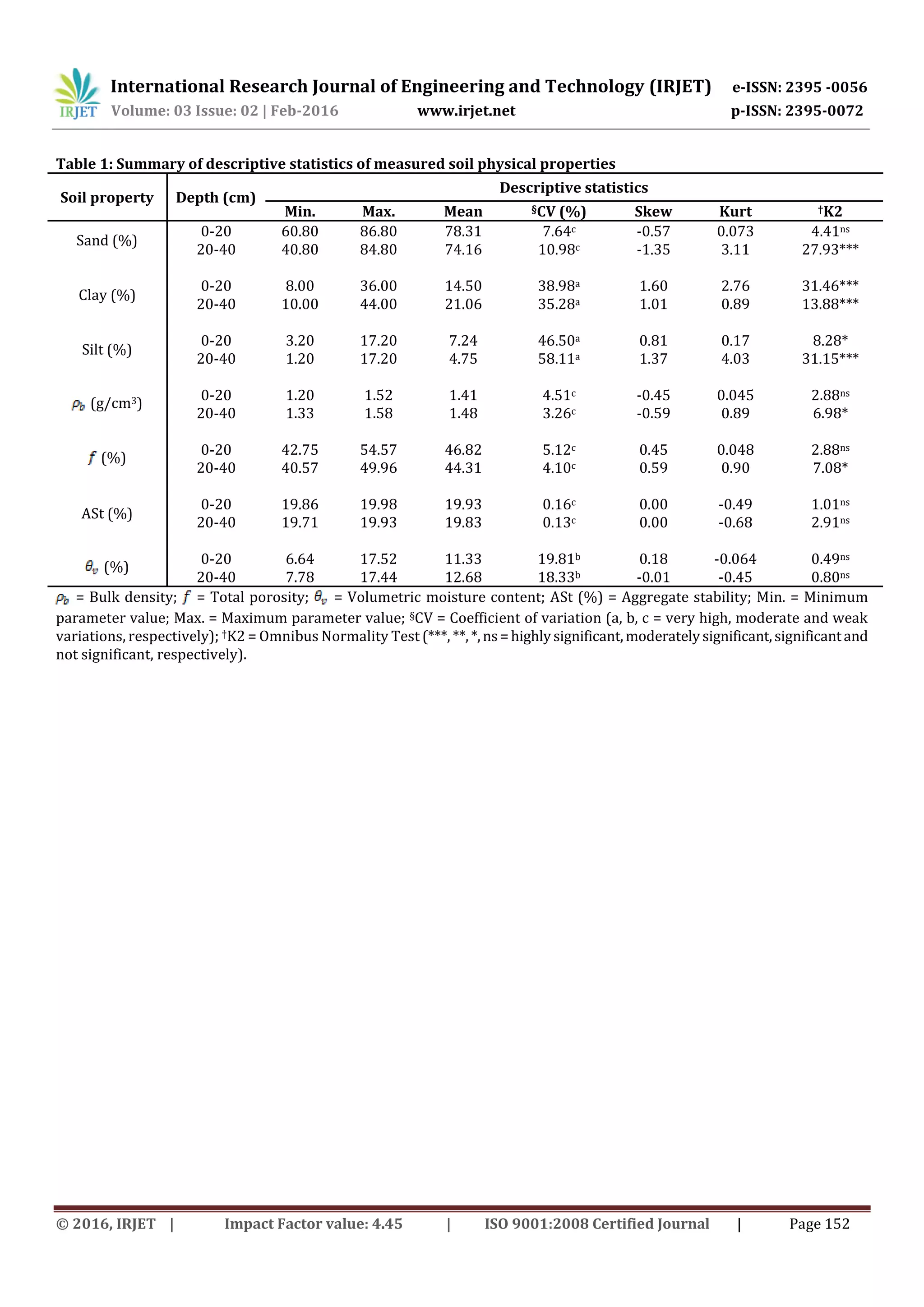
3.2.2. Spatial structure of soil structure indicators
Soil properties describing soil structure exhibited
considerable spatial variability across the field with
considerably low nugget values indicating small errors of
estimation, which could have resulted from factors such as
sampling intensity, positioning, data recording and
measurement errors. From the results, bulk density was
fitted by spherical and Gaussian models, total porosity by
linear and exponential models, and aggregate stability by
linear and spherical models for the surface and subsurface
layers, respectively as presented in Figures 2a-c. In general,
the nugget/sill ratios were described as strong to weak
spatial dependence. For instance, in the surface layer, the
strong SD (13.30%) was observed for bulk density,whereas,
aggregate stability exhibited pure nugget or very strong
spatial independence (100%). With regard to bulk density,
the values for nugget, sill, SD and rangeincreased withdepth
within the soil profile. This increase indicated higher
structured variance, nugget effect/random variability and
range with increase in depth, which may reflect a
depositional event or a series of depositional events.
Contrary to this, Tsegaye and Hill [24] found lower
structural variability in the surface bulk density, as judged
from a higher nugget (0.003) and lower sill (0.004), which
implied that 75% of the total variability was attributable to
the nugget within a range of 22 m. This lower range could
have been due to a much smaller sampling interval of 1 m in

a relatively small area (45 x 37 m) as compared to the 75 x
40 m area with 10 x 5 m sampling intervals used in this
study.
Figure 2a: Best-fitted isotropic semivariogram for
bulk density for the surface and subsurface layers
Figure 2b: Best-fitted isotropic semivariogram for
total porosity for the surface and subsurface layers

Figure 2c: Best-fitted isotropic semivariogram for
aggregate stability for the surface and subsurface
layers
3.2.3. Spatial structure of moisture content
The semivariogram functions for volumetric moisture
content were exponential and spherical the surface and
subsurface layers, respectively as shown in Figure 3. In the
surface layer, a fairly higher nuggetandsill,andhigher range
were observed in contrast to the subsurface layer, with
exception of the range. These observations were indicative
of small estimated errors, which occurred in the subsurface
layer. The range in the subsurface layer also showed that
moisture content was spatially correlated at a very short
distance, which implied that sampling for moisture
measurements should be within a distance of 0.30 m. The
nugget/sill ratios for both layers exhibited strong spatial
dependence. However, the results showed that the surface
layer was fairly strongly dependent at a longer distance,and
a shorter distance for the subsurface layer. This indicates
that future sampling for soil moisture measurements (by
volume) should be within a maximum distance of 237.30 m.
Figure 3: Best-fitted isotropic semivariogram for
volumetric moisture content for the surface and
subsurface layers
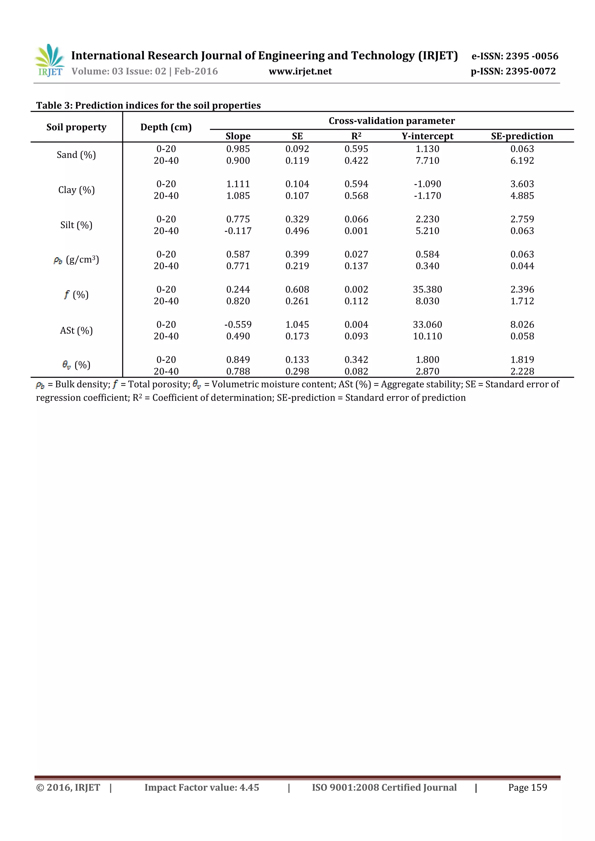
3.3. Kriging and cross-validation
The real output of the geostatistical processismapsshowing
the spatial distribution of the measured properties. The
parameters of the best-fit semivariogram models were used
for Kriging to produce these spatial distribution maps of the
soil physical properties considered in this study. Thus, the
parameters of the selected models were used to provide
estimates of the soil properties at unsampled locations
within the field. The observed values for the sampling
locations were plotted against their predicted values from
the spatial maps. The associated relative prediction indices
for the various soil properties from the contour maps are
presented in Table 3. From the Kriged maps (Figures 4-6),
regions with white colours always represented zones with
higher parameter values. The existence of minor bordered
surfaces of different colours also indicate high resolution of
the maps given by the high measuring density. Therefore,
these maps have greater resolution than mapspresentedfor
mapping units,indicatingthatverydetailedobservationscan
be made on the distribution of soil properties when
considering land use [25]. On the other hand, the results
revealed that while models could be fitted to the data, the
models’ relative abilities to predict thesoil parametervalues
at unsampled locations within the field were not good.

An ideal model was expected to have a slope of 1.0, an R2 of
1.0 and Y-intercept of 0 in order to predict the right value at
every single unsampled location. However, in this study, the
prediction indices were different from the ideal values,
which indicated that the best-fit models over predicted
lower parameter values and under predicted higher ones
[26]. Since a rigorous model prediction is somewhatdifficult
to achieve, a limit of 0.75 was set for the slope to test the
strength of the prediction. Thus, the slopes were
characterized in the order of: < 0.5, between 0.5 and 0.75,
and ≥ 0.75 to describe poor, moderate and good
predictability of the models. Generally, the scatter plots of
the observed and predicted data and their spread about the
1:1 line revealed that aggregatestabilityandtotal porosityin
the surface layer, and silt content and aggregate stability in
the subsurface layer were poor.
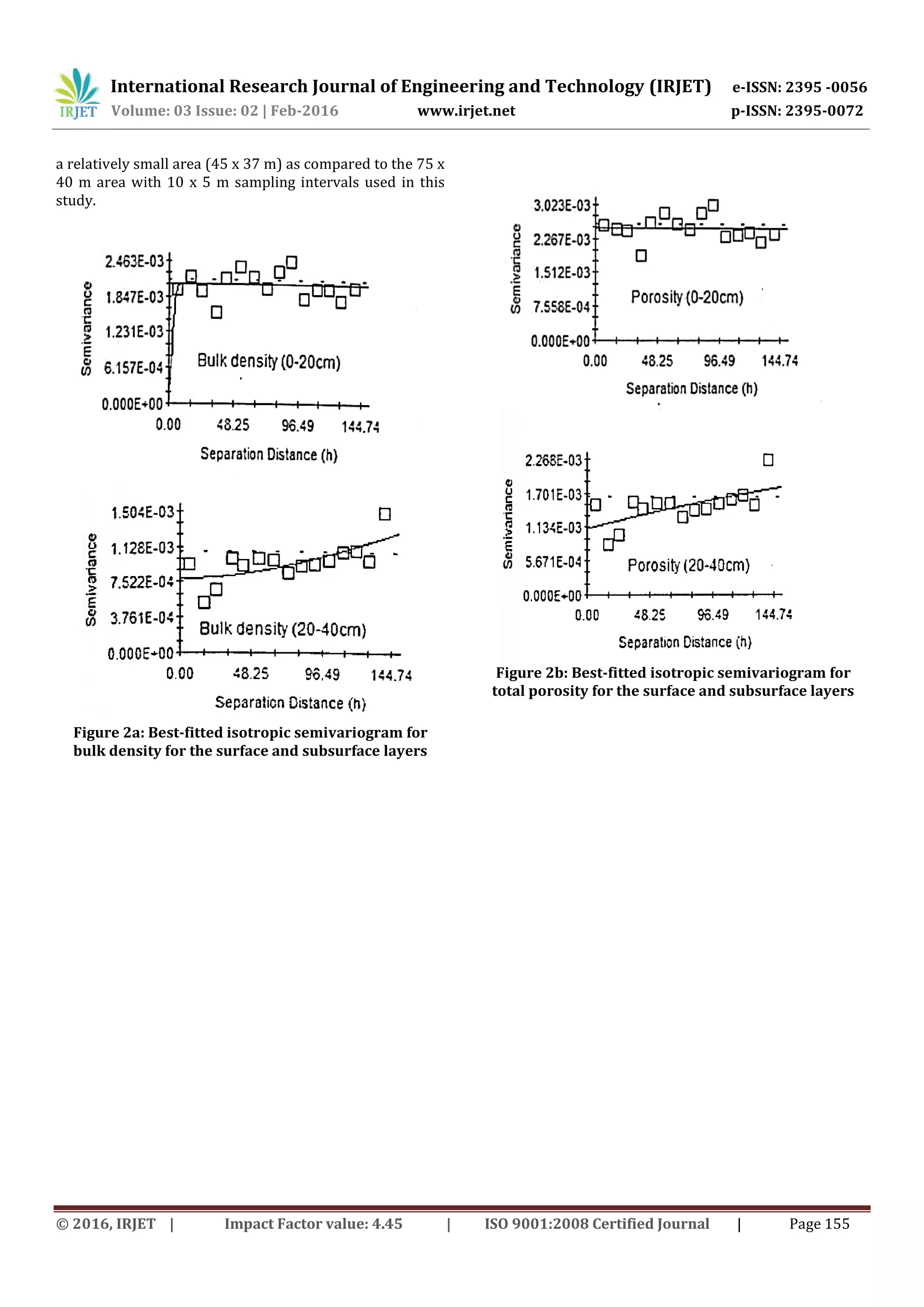
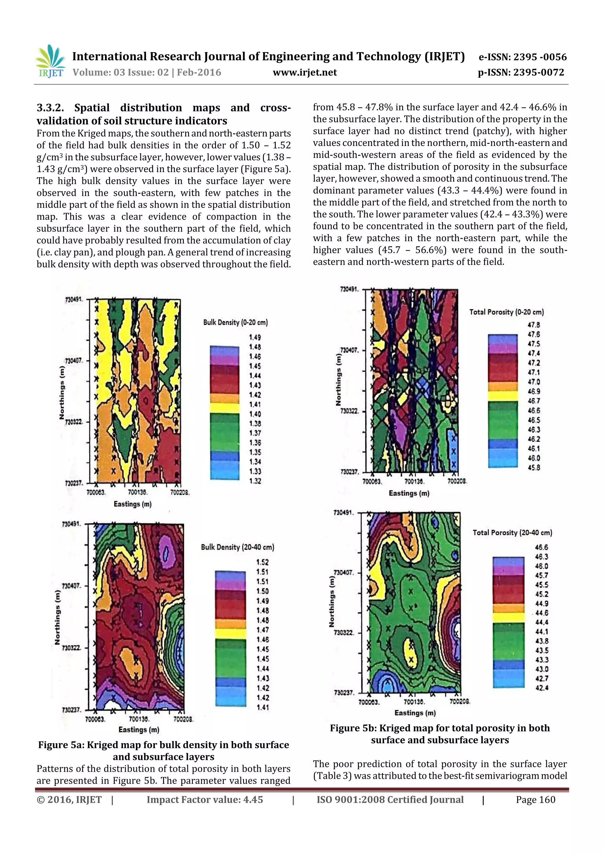
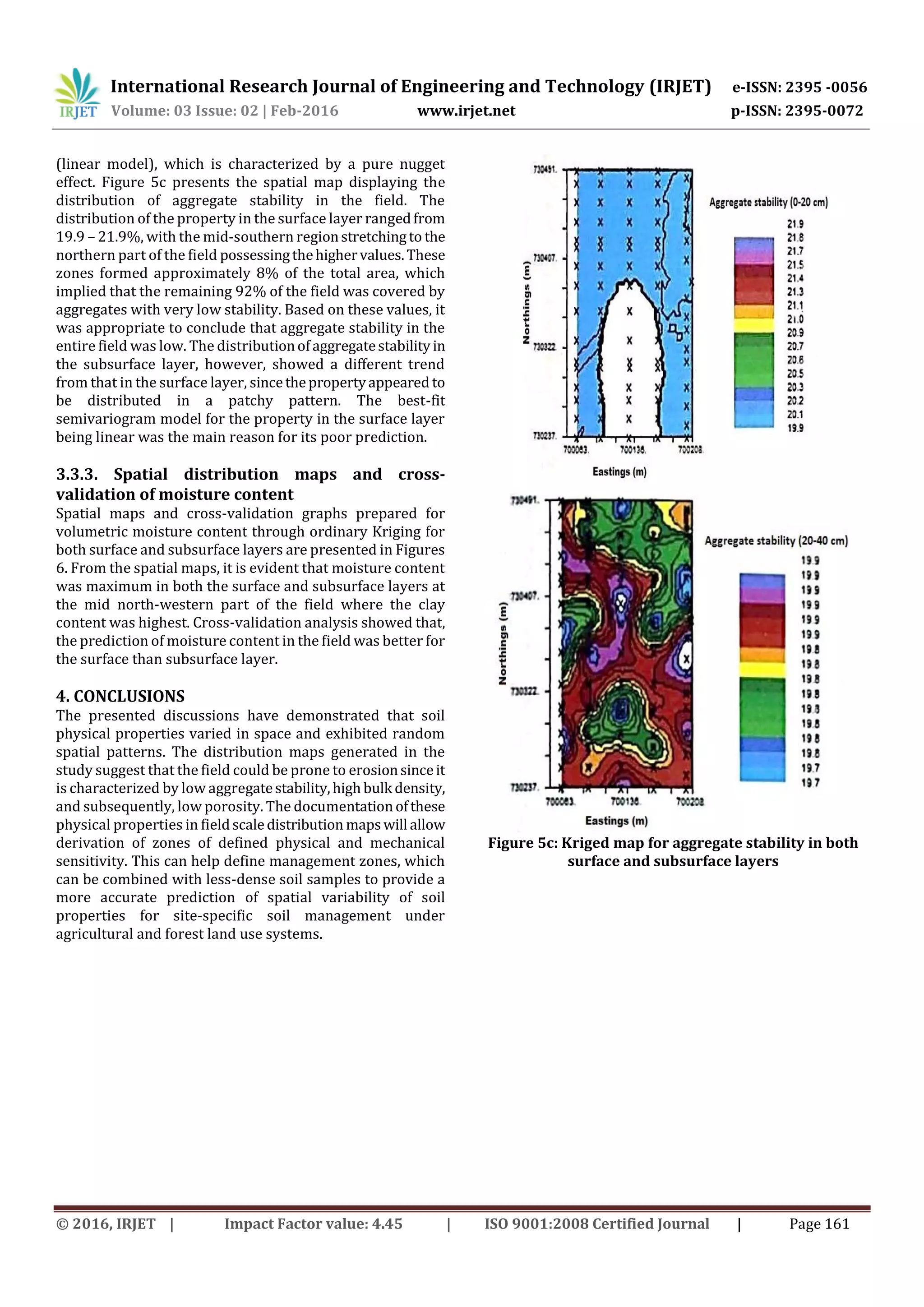
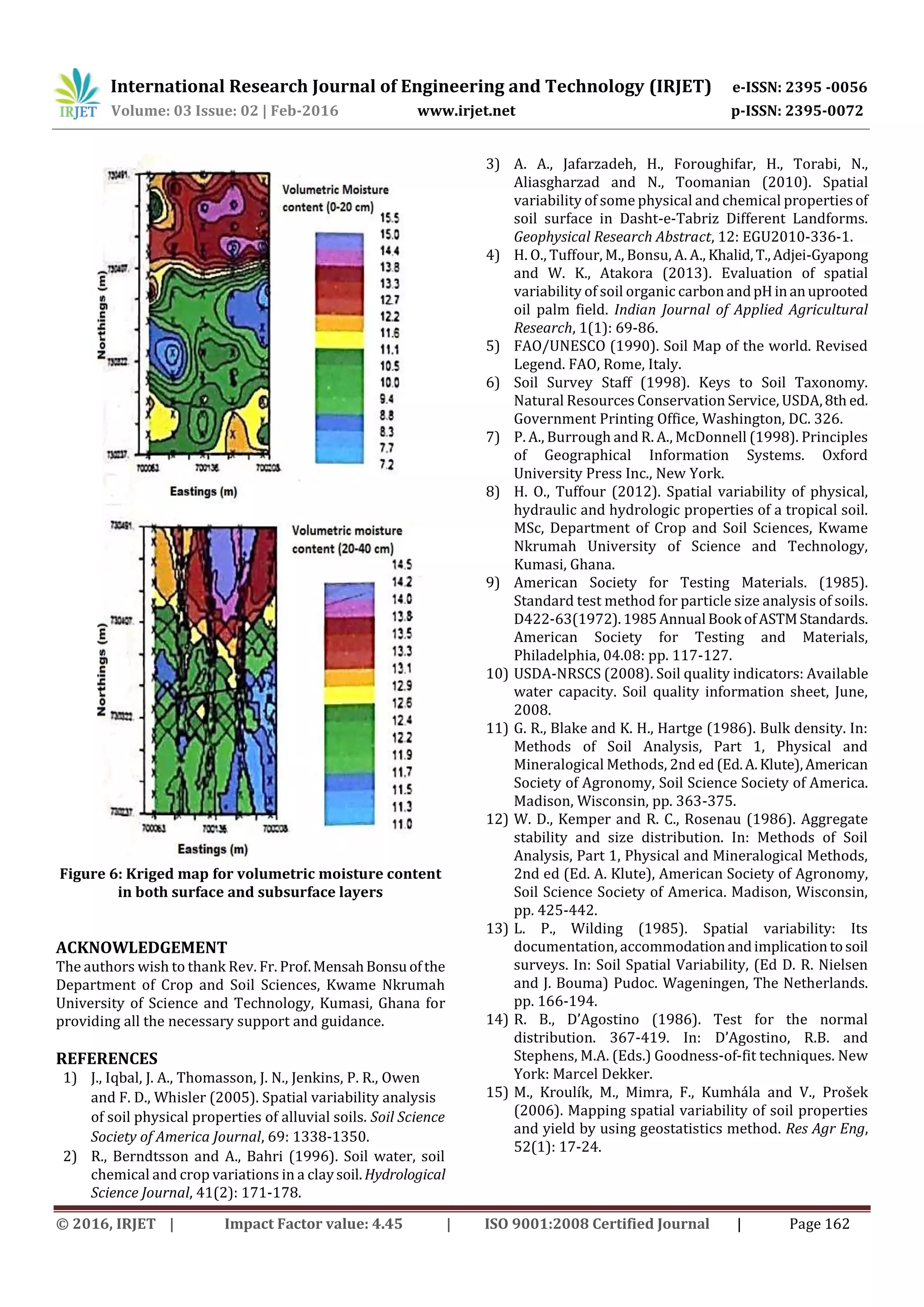
3.3.1. Spatial distribution maps and cross-
validation of particle size distribution
The spatial maps for particle size distribution (Figures 4a-c)
showed that the entire study area was characterized by
moderate to high levels of sand content, with only few
patches rich in clay content. From a detailed observation of
the spatial maps for sand content (Figure 4a), the parameter
was found to increase from the north to south in bothlayers,
but decreased with increasing depth along the profile. The
south-western, mid-eastern and south-eastern zones in the
field were observed as the areas with higher sand content in
both layers. On the contrary, significant differenceswerenot
observed in silt content in both layers (Figure 4c). The main
reason accountable for the poor prediction of silt content in
the subsurface layer was the fact it was best-fitted by linear
model, which is characterized by a pure nugget effect. The
distribution maps for clay content also revealed that the
parameter decreased from the north to south, with a fairly
uniform distribution from east to west in both layers,except
for some few patches (Figure 4b). From the spatial maps,
clay content was generally less than 22 and 30% in the
surface and subsurface layers, respectively. Thus, clay
content was generally higher in the subsurface layer than in
the surface layer.
Although the spatial variability of sand and clay contents
appeared to be more continuous in the field as depicted by
the natural behaviour of the best-fitted semivariogram
model, the distribution of areas with higher sand content
seemed to be more towards the south-western and mid-
eastern zones in both layers in the field. However, very few
clay patches appeared around the mid-western zone in the
field. Moreover, areas with lower clay contents were found
to be well distributed throughout the field. It was, therefore,
assumed that these locations with lower clay contents
resulted from the effects of erosion and lessivage.
Figure 1a: Kriged map for sand content (%) in both
surface and subsurface layers

Figure 1b: Kriged map for clay content (%) in both
Figure 1c: Kriged map for silt content (%) in both

Table 3: Prediction indices for the soil properties
Soil property Depth (cm)
Cross-validation parameter
Slope SE R2 Y-intercept SE-prediction
Sand (%)
0-20 0.985 0.092 0.595 1.130 0.063
20-40 0.900 0.119 0.422 7.710 6.192
Clay (%)
0-20 1.111 0.104 0.594 -1.090 3.603
20-40 1.085 0.107 0.568 -1.170 4.885
Silt (%)
0-20 0.775 0.329 0.066 2.230 2.759
20-40 -0.117 0.496 0.001 5.210 0.063
(g/cm3)
0-20 0.587 0.399 0.027 0.584 0.063
20-40 0.771 0.219 0.137 0.340 0.044
(%)
0-20 0.244 0.608 0.002 35.380 2.396
20-40 0.820 0.261 0.112 8.030 1.712
ASt (%)
0-20 -0.559 1.045 0.004 33.060 8.026
20-40 0.490 0.173 0.093 10.110 0.058
(%)
0-20 0.849 0.133 0.342 1.800 1.819
20-40 0.788 0.298 0.082 2.870 2.228
= Bulk density; = Total porosity; = Volumetric moisture content; ASt (%) = Aggregate stability; SE = Standard error of
regression coefficient; R2 = Coefficient of determination; SE-prediction = Standard error of prediction

validation of soil structure indicators
From the Kriged maps, the southernandnorth-easternparts
of the field had bulk densities in the order of 1.50 – 1.52
g/cm3 in the subsurface layer, however, lower values(1.38 –
1.43 g/cm3) were observed in the surface layer (Figure 5a).
The high bulk density values in the surface layer were
observed in the south-eastern, with few patches in the
middle part of the field as shown in the spatial distribution
map. This was a clear evidence of compaction in the
subsurface layer in the southern part of the field, which
could have probably resulted from the accumulation of clay
(i.e. clay pan), and plough pan. A general trend of increasing
bulk density with depth was observed throughout the field.
Figure 5a: Kriged map for bulk density in both surface
and subsurface layers
Patterns of the distribution of total porosity in both layers
are presented in Figure 5b. The parameter values ranged
from 45.8 – 47.8% in the surface layer and 42.4 – 46.6% in
the subsurface layer. The distribution of the property in the
surface layer had no distinct trend (patchy), with higher
values concentrated in the northern, mid-north-easternand
mid-south-western areas of the field as evidenced by the
spatial map. The distribution of porosity in the subsurface
layer, however, showed a smooth and continuoustrend.The
dominant parameter values (43.3 – 44.4%) were found in
the middle part of the field, and stretched from the north to
the south. The lower parameter values (42.4 – 43.3%) were
found to be concentrated in the southern part of the field,
with a few patches in the north-eastern part, while the
higher values (45.7 – 56.6%) were found in the south-
eastern and north-western parts of the field.
Figure 5b: Kriged map for total porosity in both
The poor prediction of total porosity in the surface layer
(Table 3) was attributed tothebest-fitsemivariogrammodel

(linear model), which is characterized by a pure nugget
effect. Figure 5c presents the spatial map displaying the
distribution of aggregate stability in the field. The
distribution of the property in the surface layer rangedfrom
19.9 – 21.9%, with the mid-southern regionstretchingto the
northern part of the field possessingthehighervalues.These
zones formed approximately 8% of the total area, which
implied that the remaining 92% of the field was covered by
aggregates with very low stability. Based on these values, it
was appropriate to conclude that aggregate stability in the
entire field was low. The distributionofaggregatestabilityin
the subsurface layer, however, showed a different trend
from that in the surface layer, sincethepropertyappeared to
be distributed in a patchy pattern. The best-fit
semivariogram model for the property in the surface layer
being linear was the main reason for its poor prediction.
validation of moisture content
Spatial maps and cross-validation graphs prepared for
volumetric moisture content through ordinary Kriging for
both surface and subsurface layers are presented in Figures
6. From the spatial maps, it is evident that moisture content
was maximum in both the surface and subsurface layers at
the mid north-western part of the field where the clay
content was highest. Cross-validation analysis showed that,
the prediction of moisture content in the field was better for
the surface than subsurface layer.
4. CONCLUSIONS
The presented discussions have demonstrated that soil
physical properties varied in space and exhibited random
spatial patterns. The distribution maps generated in the
study suggest that the field could be prone to erosionsinceit
is characterized by low aggregatestability,highbulk density,
and subsequently, low porosity. The documentationofthese
physical properties in fieldscaledistribution mapswill allow
derivation of zones of defined physical and mechanical
sensitivity. This can help define management zones, which
can be combined with less-dense soil samples to provide a
more accurate prediction of spatial variability of soil
properties for site-specific soil management under
agricultural and forest land use systems.
Figure 5c: Kriged map for aggregate stability in both

Figure 6: Kriged map for volumetric moisture content
in both surface and subsurface layers
ACKNOWLEDGEMENT
The authors wish to thank Rev. Fr. Prof.MensahBonsuofthe
Department of Crop and Soil Sciences, Kwame Nkrumah
University of Science and Technology, Kumasi, Ghana for
providing all the necessary support and guidance.
REFERENCES
1) J., Iqbal, J. A., Thomasson, J. N., Jenkins, P. R., Owen
and F. D., Whisler (2005). Spatial variability analysis
of soil physical properties of alluvial soils. Soil Science
Society of America Journal, 69: 1338-1350.
2) R., Berndtsson and A., Bahri (1996). Soil water, soil
chemical and crop variations in a claysoil. Hydrological
Science Journal, 41(2): 171-178.
3) A. A., Jafarzadeh, H., Foroughifar, H., Torabi, N.,
Aliasgharzad and N., Toomanian (2010). Spatial
variability of some physical and chemical propertiesof
soil surface in Dasht-e-Tabriz Different Landforms.
Geophysical Research Abstract, 12: EGU2010-336-1.
4) H. O., Tuffour, M., Bonsu, A. A., Khalid,T.,Adjei-Gyapong
and W. K., Atakora (2013). Evaluation of spatial
variability of soil organic carbon andpHinanuprooted
oil palm field. Indian Journal of Applied Agricultural
Research, 1(1): 69-86.
5) FAO/UNESCO (1990). Soil Map of the world. Revised
Legend. FAO, Rome, Italy.
6) Soil Survey Staff (1998). Keys to Soil Taxonomy.
Natural Resources Conservation Service, USDA,8th ed.
Government Printing Office, Washington, DC. 326.
7) P. A., Burrough and R. A., McDonnell (1998). Principles
of Geographical Information Systems. Oxford
University Press Inc., New York.
8) H. O., Tuffour (2012). Spatial variability of physical,
hydraulic and hydrologic properties of a tropical soil.
MSc, Department of Crop and Soil Sciences, Kwame
Nkrumah University of Science and Technology,
Kumasi, Ghana.
9) American Society for Testing Materials. (1985).
Standard test method for particle size analysis of soils.
D422-63(1972).1985Annual Book ofASTMStandards.
American Society for Testing and Materials,
Philadelphia, 04.08: pp. 117-127.
10) USDA-NRSCS (2008). Soil quality indicators: Available
water capacity. Soil quality information sheet, June,
2008.
11) G. R., Blake and K. H., Hartge (1986). Bulk density. In:
Methods of Soil Analysis, Part 1, Physical and
Mineralogical Methods, 2nd ed (Ed.A.Klute),American
Society of Agronomy, Soil Science Society of America.
Madison, Wisconsin, pp. 363-375.
12) W. D., Kemper and R. C., Rosenau (1986). Aggregate
stability and size distribution. In: Methods of Soil
Analysis, Part 1, Physical and Mineralogical Methods,
2nd ed (Ed. A. Klute), American Society of Agronomy,
Soil Science Society of America. Madison, Wisconsin,
pp. 425-442.
13) L. P., Wilding (1985). Spatial variability: Its
documentation, accommodationandimplicationtosoil
surveys. In: Soil Spatial Variability, (Ed D. R. Nielsen
and J. Bouma) Pudoc. Wageningen, The Netherlands.
pp. 166-194.
14) R. B., D’Agostino (1986). Test for the normal
distribution. 367-419. In: D’Agostino, R.B. and
Stephens, M.A. (Eds.) Goodness-of-fit techniques. New
York: Marcel Dekker.
15) M., Kroulík, M., Mimra, F., Kumhála and V., Prošek
(2006). Mapping spatial variability of soil properties
and yield by using geostatistics method. Res Agr Eng,
52(1): 17-24.

16) C. A., Cambardella and D. K., Karlen (1999). Spatial
analysis of soil fertility parameters. Precision
Agriculture, 1: 5-14.
17) P., Santra, U. K., Chopra and D., Chakraborty (2008).
Spatial variability of soil properties and its application
in predicting surface mapof hydraulic parametersinan
agricultural farm. Current Science, 95(7): 937-945.
18) E. L., Aksakal and T., Öztaş (2010). Changes in
distribution patterns of soil penetration resistance
within a silage-corn field following the use of heavy
harvesting equipment. Turkish Journal of Agriculture
and Forestry, 34: 173-179.
19) S. G., Reynolds (1970). The gravimetric method of soil
moisture determination, I: A study of equipment and
methodological problems. Hydrology, 11: 258-273.
20) E., Mapfumo, D. S., Chanasky and C. L. A., Chaikowsky
(2006). Stochastic simulation of soil water status on
reclaimed land in northern Alberta. Journal of Spatial
Hydrology, 6(1): 34-44.
21) A. W., Western, S., Zhou, R. B., Grayson, T. A., McMahon,
G., Blöschl, and D. J., Wilson (2004). Spatial correlation
of soil moisture in small catchments and its
relationship to dominant spatial hydrological
processes. Journal of Hydrology, 286: 113-134.
22) S. K., Balasundram, O. H., Ahmed, M. H., Harun, M. H. A.,
Husni and M. C., Law (2009). Spatial variability of soil
organic carbon in palm oil. International Journal of Soil
Science, 4(4): 93-103.
23) P., Goovaerts (1997). Geostatistics from natural
resource evaluation. Oxford University Press, New
York.
24) T., Tsegaye and R. L., Hill (1998). Intensive tillage
effects on spatial variability of soil physical properties.
Soil Science, 163: 143-154.
25) L., Cruz-Rodriguez (2004). Soil organic carbon and
nitrogen distribution in a tropical watershed. MSc.
Thesis. University of Puerto Rico, Mayagüez campus.
26) S., Brouder, B., Hofmann and H. F. J., Reetz (2001).
Evaluating spatial variability of soil parameters for
input management. Better Crops, 85(2): 8-11.

Mapping spatial variability of soil physical properties for site-specific management

More Related Content

What's hot

Similar to Mapping spatial variability of soil physical properties for site-specific management

More from IRJET Journal

Recently uploaded

Mapping spatial variability of soil physical properties for site-specific management