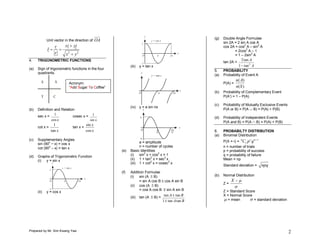
This document provides notes and formulae on additional mathematics for Form 5. It covers topics such as progressions, integration, vectors, trigonometric functions, and probability. For progressions, it defines arithmetic and geometric progressions and gives the formulas for calculating the nth term and sum of terms. For integration, it provides rules and formulas for integrating polynomials, trigonometric functions, and expressions with ax+b. It also defines vectors and their operations including vector addition and subtraction. Other sections cover trigonometric functions, their definitions, relationships and graphs, as well as probability topics such as calculating probabilities of events and distributions like the binomial.

1. NOTES AND FORMULAE ADDITIONAL MATHEMATICS FORM 5
1. PROGRESSIONS (iii)
(a) Arithmetic Progression b c c
Tn = a + (n – 1)d
n

a

f ( x )dx  f ( x )dx 
b
 f ( x)dx
a
Sn = [2a  ( n  1)d ]
2 (d) Area under a curve
n   
 
= [ a  Tn ] AC  AB  BC
2
(b) Geometric Progression
(b) A, B and C are collinear if
Tn = ar
n–1

 
n AB   BC where  is a constant.
Sn 
a (1  r ) 
 
1 r AB and PQ are parallel if
Sum to infinity
 
b b
PQ   AB where  is a constant.
a
S 
1 r
A=

a
ydx A=
 xdy
a
(c) Subtraction of Two Vectors
(c) General
Tn = Sn − Sn – 1
T1 = a = S1 (e) Volume of Revolution
2. INTEGRATION
x n 1   
  
(a)
 xn dx  c
n 1 AB  OB  OA
(ax  b) n 1 (d) Vectors in the Cartesian Plane
(b)
 ( ax  b) n dx  c
(n  1)a
(c) Rules of Integration:
b b b b
V   y 2 dx
 V   x 2 dy

(i)
 nf ( x)dx  n f ( x)dx
a a a a
a b
3. VECTORS 

(ii)
 f ( x)dx   f ( x)dx
b a
(a) Triangle Law of Vector Addition OA  xi  yj
 
Magnitude of
 
 
OA  OA  x 2  y 2
Prepared by Mr. Sim Kwang Yaw 1

2. (g) Double Angle Formulae
Unit vector in the direction of OA sin 2A = 2 sin A cos A
r xi  yj 2
cos 2A = cos A – sin A
2
r    
ˆ 2
= 2cos A – 1
 r x2  y 2 2
= 1 – 2sin A

4. TRIGONOMETRIC FUNCTIONS 2 tan A
tan 2A =
(iii) y = tan x 1  tan 2 A
(a) Sign of trigonometric functions in the four
5. PROBABILITY
quadrants.
(a) Probability of Event A
n( A)
Acronym: P(A) =
“Add Sugar To Coffee” n( S )
(b) Probability of Complementary Event
P(A) = 1 – P(A)
(c) Probability of Mutually Exclusive Events
(iv) y = a sin nx
(b) Definition and Relation P(A or B) = P(A  B) = P(A) + P(B)
sec x =
1 cosec x = 1 (d) Probability of Independent Events
cos x sin x
P(A and B) = P(A  B) = P(A) × P(B)
1 sin x
cot x = tan x =
tan x cos x 6. PROBABILTY DISTRIBUTION
(a) Binomial Distribution
(c) Supplementary Angles n
P(X = r) = Cr p q
r n r
o
sin (90 − x) = cos x a = amplitude
o
cot (90 – x) = tan x n = number of cycles n = number of trials
(e) Basic Identities p = probability of success
2 2
(d) Graphs of Trigonometric Function (i) sin x + cos x = 1 q = probability of failure
2 2
(i) y = sin x (ii) 1 + tan x = sec x Mean = np
2 2
(iii) 1 + cot x = cosec x
Standard deviation = npq
(f) Addition Formulae
(i) sin (A  B) (b) Normal Distribution
= sin A cos B  cos A sin B X 
Z=
(ii) cos (A  B) 
= cos A cos B  sin A sin B Z = Standard Score
(ii) y = cos x
(iii) tan (A  B) = tan A  tan B X = Normal Score
1  tan A tan B  = mean  = standard deviation
Prepared by Mr. Sim Kwang Yaw 2

3. (b) Condition and Implication:
(a) Normal Distribution Graph Condition Implication
Returns to O s=0
To the left of O s<0
To the right of O s>0
Maximum/Minimum ds = 0
displacement dt
Initial velocity v when t = 0
Uniform velocity a=0
Moves to the left v<0
Moves to the right v>0
Stops/change v=0
direction of motion
P(Z < k) = 1 – P(Z > P(Z < -k) = P(Z > k) Maximum/Minimum dv = 0
k) velocity dt
Initial acceleration a when t = 0
Increasing speed a>0
Decreasing speed a<0
(c) Total Distance Travelled in the Period
P(Z > -k) = 1 – P(Z < - P(a < Z < b) 0 ≤ t ≤ b Second
k) = 1 – P(Z > k) = P(Z > a) – P(Z > b) (i) If the particle does not stop in the
period of 0 ≤ t ≤ b seconds
Total distance travelled
= displacement at t = b second
(ii) If the particle stops in t = a second
when t = a is in the interval of 0 ≤ t ≤
P(-b < Z < -a) = P(a < P(- b < Z < a) b second,
Z < b) = P(Z > a) – = 1 – P(z > b) – P(Z > Total distance travelled in b second
P(Z > b) a) = Sa  S0  Sb  Sa
7. MOTION ALONG A STRAIGHT LINE
(a) Relation Between Displacement,
Velocity and Acceleration
 vdt  adt
Prepared by Mr. Sim Kwang Yaw 3