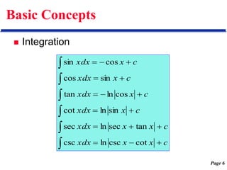
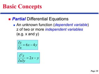
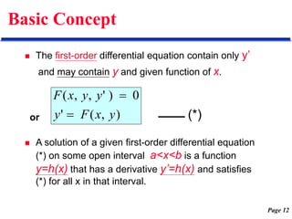
This document provides an outline and overview of concepts related to first-order differential equations. It discusses basic concepts such as differentiation, integration, orders of differential equations, and general vs. particular solutions. It also covers specific types of first-order differential equations like separable, exact, and linear differential equations. Methods for solving these types of equations are presented, including separation of variables, substitution, integrating factors, and finding general and particular solutions. Examples of applying these concepts and solution methods are provided.

1. 王 俊 鑫 (Chun-Hsin Wang)
中華大學 資訊工程系
Fall 2002
Chap 1 First-Order
Differential Equations

2. Page 2
Outline
 Basic Concepts
 Separable Differential Equations
 substitution Methods
 Exact Differential Equations
 Integrating Factors
 Linear Differential Equations
 Bernoulli Equations

3. Page 3
Basic Concepts
 Differentiation
x
e
x
x
x
a
a
a
e
e
nx
x
a
a
x
x
x
x
n
n
log
)
(log
1
)
(ln
ln
)
(
)
(
)
( 1









 
x
x
x
x
x
x
x
x
x
x
x
x
x
x
cot
csc
)
(csc
tan
sec
)
(sec
csc
)
(cot
sec
)
(tan
sin
)
(cos
cos
)
(sin
2
2
















4. Page 4
Basic Concepts
 Differentiation
x
x
x
x
sinh
)
(cosh
cosh
)
(sinh




2
1
2
1
2
1
2
1
1
1
)
(cot
1
1
)
(tan
1
1
)
(cos
1
1
)
(sin
x
x
x
x
x
x
x
x



















5. Page 5
Basic Concepts
 Integration
c
a
a
dx
a
c
e
dx
e
c
x
dx
x
dx
x
c
n
x
dx
x
x
x
x
x
n
n

















ln
ln
1
1
1
1



















vdx
u
uv
dx
v
u
vdu
uv
udv
udx
c
cudx
vdx
udx
dx
v
u )
(

6. Page 6
Basic Concepts
 Integration
c
x
x
xdx
c
x
x
xdx
c
x
xdx
c
x
xdx
c
x
xdx
c
x
xdx






















cot
csc
ln
csc
tan
sec
ln
sec
sin
ln
cot
cos
ln
tan
sin
cos
cos
sin

7. Page 7
Basic Concepts
 Integration
c
a
x
dx
a
x
c
a
x
dx
a
x
c
a
x
dx
x
a
c
a
x
a
dx
a
x




















1
2
2
1
2
2
1
2
2
1
2
2
cosh
1
sinh
1
sin
1
tan
1
1

8. Page 8
Basic Concepts
 ODE vs. PDE
 Dependent Variables vs. Independent
Variables
 Order
 Linear vs. Nonlinear
 Solutions

9. Page 9
Basic Concepts
 Ordinary Differential Equations
 An unknown function (dependent variable) y
of one independent variable x
x
dx
dy
y cos



0
4 


 y
y
2
2
2
)
2
(
2 y
x
y
e
y
y
x x










10. Page 10
Basic Concepts
 Partial Differential Equations
 An unknown function (dependent variable)
z of two or more independent variables
(e.g. x and y)
y
x
x
z
4
6 



y
x
y
x
z





2
2

11. Page 11
Basic Concepts
 The order of a differential equation is
the order of the highest derivative that
appears in the equation.
0
)
( 2
2
3






 y
n
x
y
x
y
x Order 2
2
2
1
y
x
dx
dy

 Order 1
1
)
( 4
3
2
2

 y
dx
y
d
Order 2

12. Page 12
Basic Concept
 The first-order differential equation contain only y’
and may contain y and given function of x.
 A solution of a given first-order differential equation
(*) on some open interval a<x<b is a function
y=h(x) that has a derivative y’=h(x) and satisfies
(*) for all x in that interval.
)
,
(
'
0
)
'
,
,
(
y
x
F
y
y
y
x
F


or (*)

13. Page 13
Basic Concept
 Example : Verify the solution
x
2
y
2y
xy'



14. Page 14
Basic Concepts
 Explicit Solution
 Implicit Solution
)
(x
h
y 
0
)
,
( 
y
x
H

15. Page 15
Basic Concept
 General solution vs. Particular solution
 General solution
 arbitrary constant c
 Particular solution
 choose a specific c
,....
2
,
3
'






c
c
sinx
y
cosx
y

16. Page 16
Basic Concept
 Singular solutions
 Def : A differential equation may sometimes have an
additional solution that cannot be obtained from the
general solution and is then called a singular
solution.
 Example
The general solution : y=cx-c2
A singular solution : y=x2/4
0
' 

 y
xy
y'
2

17. Page 17
Basic Concepts
 General Solution
 Particular Solution for y(0)=2 (initial condition)
kt
ce
t
y 
)
(
kt
e
t
y 2
)
( 
ky
y 


18. Page 18
Basic Concept
 Def: A differential equation together
with an initial condition is called an
initial value problem
0
0)
(
),
,
(
' y
x
y
y
x
f
y 


19. Page 19
Separable Differential Equations
 Def: A first-order differential equation of
the form
is called a separable differential
equation
dx
x
f
dy
y
g
f(x)
g(y)y
)
(
)
(
'



20. Page 20
Separable Differential Equations
 Example :
Sol:
0
4
9 

 x
y
y

21. Page 21
Separable Differential Equations
 Example :
Sol:
2
1 y
y 



22. Page 22
Separable Differential Equations
 Example :
Sol:
ky
y 


23. Page 23
Separable Differential Equations
 Example :
Sol:
1
)
0
(
,
2 


 y
xy
y

24. Page 24
Separable Differential Equations
 Substitution Method:
A differential equation of the form
can be transformed into a separable
differential equation
)
(
x
y
g
y 


25. Page 25
Separable Differential Equations
 Substitution Method:
ux
y  u
x
u
y 



x
dx
u
u
g
du
u
u
g
x
u
u
g
u
x
u










)
(
)
(
)
(

26. Page 26
Separable Differential Equations
 Example :
Sol:
2
2
2 x
y
y
xy 


cx
y
x
x
c
x
y
x
c
u
c
x
c
x
u
x
dx
u
udu
u
u
u
x
u
y
x
x
y
xy
x
xy
y
y
x
y
y
xy








































2
2
2
2
1
1
2
2
2
2
2
2
1
1
1
ln
ln
)
1
ln(
1
2
)
1
(
2
1
)
(
2
1
2
2
2

27. Page 27
Separable Differential Equations
 Exercise 1
2
01
.
0
1 y
y 


2
/
xy
y 

y
y
y
x 

 2
2
)
2
(
,
0
' 


 y
y
xy

28. Page 28
Exact Differential Equations
 Def: A first-order differential equation of
the form
is said to be exact if
0
)
,
(
)
,
( 
 dy
y
x
N
dx
y
x
M
x
y
x
N
y
y
x
M



)
,
(
)
,
(

29. Page 29
Exact Differential Equations
 Proof:
0
)
,
(
)
,
(
0
)
,
(









dy
y
x
N
dx
y
x
M
dy
y
u
dx
x
u
y
x
du
x
y
x
N
y
y
x
M
y
x
y
x
u






 )
,
(
)
,
(
)
,
(

30. Page 30
Exact Differential Equations
 Example :
Sol:
0
)
3
(
)
3
( 3
2
2
3



 dy
y
y
x
dx
xy
x
Exact
xy
x
N
y
M
xy
x
y
y
x
xy
y
xy
x
,
6
6
3
6
3
3
2
2
3














31. Page 31
Exact Differential Equations
Sol:
)
(
2
3
4
1
)
(
)
3
(
)
(
2
2
4
2
3
y
k
y
x
x
y
k
dx
xy
x
y
k
Mdx
u










1
4
3
2
2
4
)
(
3
)
(
3
c
y
y
k
y
y
x
N
dy
y
dk
y
x
y
u











32. Page 32
Exact Differential Equations
Sol:
c
y
y
x
x
y
x
u 


 )
6
(
4
1
)
,
( 4
2
2
4

33. Page 33
Exact Differential Equations
 Example
3
)
0
(
0
)
sinh
(cos
)
cosh
(sin



y
dy
y
x
dx
y
x

34. Page 34
Non-Exactness
 Example : 0


 xdy
ydx

35. Page 35
Integrating Factor
 Def: A first-order differential equation of the form
is not exact, but it will be exact if multiplied by
F(x, y)
then F(x,y) is called an integrating factor of this
equation
0
)
,
(
)
,
( 
 dy
y
x
Q
dx
y
x
P
0
)
,
(
)
,
(
)
,
(
)
,
( 
 dy
y
x
Q
y
x
F
dx
y
x
P
y
x
F

36. Page 36
Exact Differential Equations
 How to find integrating factor
 Golden Rule
x
x
y
y FQ
Q
F
FP
P
F
Exact
x
FQ
y
FP
FQdy
FPdx












,
0
)
(
1
1
0
Let
x
y
x
y
Q
P
Q
dx
dF
F
FQ
Q
dx
dF
FP
P
F(x)
F









37. Page 37
Exact Differential Equations
 Example :
Sol:
0


 xdy
ydx
Exact
x
N
x
y
M
dy
x
dx
x
y
x
xdy
ydx
x
F
,
1
1
1
2
2
2
2














38. Page 38
Exact Differential Equations
Sol:
cx
y
c
x
y
x
y
d
dy
x
dx
x
y







 0
)
(
1
2

39. Page 39
Exact Differential Equations
 Example :
2
)
2
(
0
)
cos(
)
sin(
2 2
2




y
dy
y
xy
dx
y

40. Page 40
Exact Differential Equations
 Exercise 2
0
2 2

 dy
x
xydx 0
)
( 2
2





d
r
rdr
e
x
e
F
ydy
ydx 

 ,
0
cos
sin
b
a
y
x
F
xdy
b
ydx
a 



 ,
0
)
1
(
)
1
(
0
)
1
(
)
1
( 


 dy
x
dx
y

41. Page 41
Linear Differential Equations
 Def: A first-order differential equation is
said to be linear if it can be written
 If r(x) = 0, this equation is said to be
homogeneous
)
(
)
( x
r
y
x
p
y 



42. Page 42
Linear Differential Equations
 How to solve first-order linear homogeneous
ODE ?
Sol:
0
)
( 

 y
x
p
y




 















dx
x
p
c
dx
x
p
c
dx
x
p
ce
e
e
e
y
c
dx
x
p
y
dx
x
p
y
dy
y
x
p
dx
dy
)
(
)
(
)
(
1
1
1
)
(
ln
)
(
0
)
(

43. Page 43
Linear Differential Equations
 Example :
Sol:
0


 y
y
x
c
x
c
x
dx
dx
x
p
e
c
e
ce
ce
ce
ce
x
y
2
)
1
(
)
(
1
1
)
(












44. Page 44
Linear Differential Equations
 How to solve first-order linear nonhomogeneous
ODE ?
Sol:
)
(
)
( x
r
y
x
p
y 


)
(
))
(
)
(
(
)
(
1
1
0
))
(
)
(
(
)
(
)
(
x
p
x
r
y
x
p
y
Q
P
Q
dx
dF
F
dy
dx
x
r
y
x
p
x
r
y
x
p
dx
dy
x
y 














45. Page 45
Linear Differential Equations
Sol:


dx
x
p
e
x
F
)
(
)
(





 




















c
dx
r
e
e
x
y
c
dx
r
e
y
e
r
e
y
e
py
y
e
dx
x
p
dx
x
p
dx
x
p
dx
x
p
dx
x
p
dx
x
p
dx
x
p
)
(
)
(
)
(
)
(
)
(
)
(
)
(
)
(
)
(
)
(

46. Page 46
Linear Differential Equations
 Example :
Sol:
x
e
y
y 2



 
 
x
x
x
x
x
x
x
x
dx
dx
dx
x
p
dx
x
p
e
ce
c
e
e
c
dx
e
e
e
c
dx
e
e
e
c
dx
r
e
e
x
y
2
2
2
)
1
(
)
1
(
)
(
)
(
)
(











 








 












47. Page 47
Linear Differential Equations
 Example :
)
2
cos
2
2
sin
3
(
2 x
x
e
y
y x
'




48. Page 48
Bernoulli, Jocob
Bernoulli, Jocob
1654-1705

49. Page 49
Linear Differential Equations
 Def: Bernoulli equations
 If a = 0, Bernoulli Eq. => First Order
Linear Eq.
 If a <> 0, let u = y1-a
a
y
x
g
y
x
p
y )
(
)
( 


g
a
pu
a
u )
1
(
)
1
( 





50. Page 50
Linear Differential Equations
 Example :
Sol:
2
By
Ay
y 



 
A
B
ce
u
y
A
B
ce
c
dx
e
A
B
e
c
dx
Be
e
u
B
Au
u
Ay
B
Ay
By
y
y
y
u
y
y
y
u
Ax
Ax
Ax
Ax
Ax
Ax
a














































1
1
)
( 1
2
2
2
1
2
1
1

51. Page 51
Linear Differential Equations
 Exercise 3
4


 y
y kx
e
ky
y 



2
2 y
y
y 


1



 xy
xy
y
)
2
(
,
sin
3 
y
x
y
y 



52. Page 52
Summary
可分離 Separable 
變換法 Substitution 
正合 Exact 
積分因子 Integrating Factor 
線性 Linear 
柏努利 Bernoulli 
dx
x
f
dy
y
g )
(
)
( 
dx
x
f
du
u
g )
(
)
( 
0
)
,
(
)
,
( 
 dy
y
x
N
dx
y
x
M
0

 FQdy
FPdx
)
(
)
( x
r
y
x
p
y 


a
y
x
g
y
x
p
y )
(
)
( 



53. Page 53
Orthogonal Trajectories of
Curves
 Angle of intersection of two curves is
defined to be the angle between the
tangents of the curves at the point of
intersection
 How to use differential equations for
finding curves that intersect given
curves at right angles ?

54. Page 54
How to find Orthogonal Trajectories
 1st Step: find a differential equation
for a given cure
 2nd Step: the differential equation of the
orthogonal trajectories to be found
 3rd step: solve the differential equation
as above ( in 2nd step)
)
,
( y
x
f
y 
)
,
( y
x
f
y' 
)
,
(
1
y
x
f
y' 


55. Page 55
Orthogonal Trajectories of Curves
 Example: given a curve y=cx2, where c
is arbitrary. Find their orthogonal
trajectories.
Sol:

56. Page 56
Existance and Uniqueness of Solution
 An initial value problem may have no
solutions, precisely one solution, or
more than one solution.
 Example
1
)
0
(
,
0
' 

 y
y
y
1
)
0
(
,
' 
 y
x
y
1
)
0
(
,
1
' 

 y
y
xy
No solutions
Precisely one solutions
More than one solutions

57. Page 57
Existence and uniqueness theorems
 Problem of existence
 Under what conditions does an initial
value problem have at least one
solution ?
 Existence theorem, see page 53
 Problem of uniqueness
 Under what conditions does that the
problem have at most one solution ?
 Uniqueness theorem, see page54