The document provides step-by-step instructions for creating a 3D solid model of a W16x50 steel beam in ANSYS Workbench. It describes sketching the cross-section profile on the xy-plane, adding symmetry and dimensional constraints, and then extruding the sketch to generate the full 3D beam geometry 10 feet in length. Additional techniques demonstrated include copying/pasting sketches, trimming excess lines, adding fillets, and moving dimensional values. The overall purpose is to practice basic sketching skills needed for geometry creation in simulations.

1. Finite Element
Simulations with
ANSYS Workbench 14
Theory, Applications, Case Studies
® ™
Huei-Huang Lee
www.SDCpublications.com
Better Textbooks. Lower Prices.SDCP U B L I C A T I O N S
Schroff Development Corporation
Supplemental
Files
Tutorial files on
enclosed DVD

2. Visit the following websites to learn more about this book:

3. Chapter 2 Sketching 53
Chapter 2
Sketching
A simulation project starts with the creation of a geometric model. To be successful on simulations, an engineer has to
be pro4cient at geometric modeling 4rst. In a simulation project, it is not uncommon to take majority of human-hours
to create a geometric model; it is particularly true in a 3D simulation.
A complex 3D geometry can be viewed as a series of boolean operations (unions, subtractions, etc.) of simpler
3D solid bodies. Each solid body is often created by 4rst drawing a sketch on a plane; the sketch is then used to
generate the 3D solid body by using a tool such as <Extrude>, <Revolve>, <Sweep>, etc. In turn, to be pro4cient at
3D bodies creation, an engineer has to be pro4cient at sketching 4rst.
Purpose of the Chapter
The purpose of this chapter is to provide exercises for the students so that they can be pro4cient at sketching using
<DesignModeler>. Pro4les of 4ve mechanical parts are created in this chapter. Each sketch is used to generate a 3D
model using a 3D tool of either <Extrude> or <Revolve>. The use of the 3D tools is trivial enough that we should be
able to focus on the 2D sketches.
About Each Section
Each sketch of a mechanical part will be completed in a section. Sketches in the 4rst two sections are guided in a
step-by-step fashion. Section 1 sketches a cross section of W16x50; the cross section is then extruded to generate a
3D beam. Section 2 sketches a triangular plate; the sketch is then extruded to generate a 3D solid model.
Section 3 does not mean to provide a hands-on case. It overviews the sketching tools in a systematic way,
attempting to complement what were missed in the 4rst two sections.
Sections 4, 5, and 6 provide three cases for more exercises. We will present in a not-so-step-by-step fashion; we
purposely leave some room for the students to 4gure out the details.

4. 54 Chapter 2 Sketching
Section 2.1
Step-by-Step: W16x50 Beam
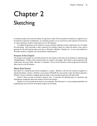
In this section, we will create a 3D solid body for a steel beam.
The steel beam has a W16x50 cross-section [1-4] and a length of
10 ft.
2.1-1 About the W16x50 Beam
W16x50
16.25"
.628"
.380"
7.07"
R.375"
[1] Wide-9ange
I-shape section.
[2] Nominal
depth 16 in.
[3] Weight 50
lb/ft.
[4] Detail
dimensions.
[2] <Workbench
GUI> shows up.
[3] Click the plus sign (+) to
expand <Component
Systems>. The plus sign
becomes minus sign.
[4] Double-click
<Geometry> to
create a system in
<Project
Schematic>.
[6] Double-click
<Geometry> to start
up <DesignModeler>,
the geometry editor.
[5]You may click
here to show the
messages from
ANSYS Inc. To hide
the message, click
again.
[1] Launch
Workbench.
2.1-2 Start Up <DesignModeler>

5. Section 2.1 Step-by-Step: W16x50 Beam 55
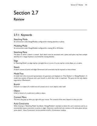
Notes: In this book, when a circle is used with a speech bubble, it is to indicate that mouse or keyboard ACTIONS
are needed in that step [1, 3, 4, 6, 8, 9]. A circle may be @lled with white color [1, 4, 6] or un@lled [3, 8, 9]. A speech
bubble without a circle [2, 7] or with a rectangle [5] is used for commentary only, i.e., no mouse or keyboard actions
are needed.
2.1-3 Draw a Rectangle on <XYPlane>
[9] Click <OK>. Note
that, after entering
<DesignModeler>, the
length unit cannot be
changed anymore.
[8] Select <Inch> as
length unit.
[7]
<DesignModeler>
shows up.
[1] By default,
<XYPlane> is the
current sketching
plane.
[2] Click to switch
to <Sketching
Mode>.
[4] Click
<Rectangle>
tool.
[3] Click <Look At
Face/Plane/Sketch>
to rotate the view
angle so that you
look at <XYPlane>.
[5] Draw a
rectangle (using
click-and-drag)
roughly like this.

6. 56 Chapter 2 Sketching
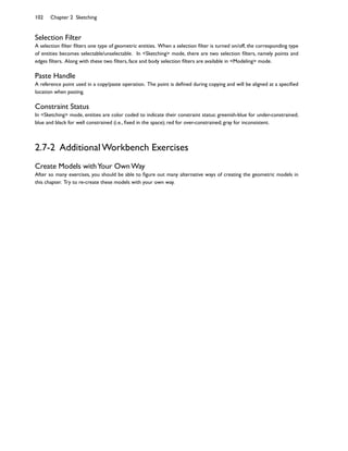
Impose symmetry constraints...
[6] Click
<Constraints>
toolbox.
[8] Click
<Symmetry>
tool.
[9] Click the vertical
axis and then two
vertical lines on both
sides to make them
symmetric about the
vertical axis.
[10] Right-click
anywhere on the graphic
area to open the context
menu, and choose
<Select new symmetry
axis>.
[11] Click the
horizontal axis and
then two horizontal
lines on both sides
to make them
symmetric about
the horizontal axis.
[7] If you don't
see <Symmetry>
tool, click here to
scroll down until
you see the tool.
[12] Click
<Dimensions>
toolbox.
[13]
<General> is
the default tool.
[17] In <Details
View>, type 7.07
(in) for H1 and
16.25 (in) forV2.
[14] Click this line,
move the mouse
upward, then click again
to create H1.
[15] Click this line,
move the mouse
rightward, then click
again to createV2.
[18] Click
<Zoom to Fit>.
[16] All the lines turn to blue
color. Colors are used to
indicate the constraint status.
The blue color means a
geometric entity is well
constrained.
Specify dimensions...

7. Section 2.1 Step-by-Step: W16x50 Beam 57
2.1-4 Clean up the Graphic Area
The ruler occupies space and is sometimes annoying; let's turn it off...
Let's display dimension values (instead of names) on the graphic area...
[2] The ruler will
disappear. We turn off
the ruler to make more
space for the graphic
area. For the rest of the
book, we always leave
the ruler off.
[1] Pull-down-select
<View/Ruler> to
turn the ruler off.
[3] If you don't see
<Display> tool,
click here to scroll
all the way down
to the bottom.
[4] Click
<Display> tool.
[5] Click <Name> to
turn it off. <Value>
automatically turns on.
[6] Dimension
names are replaced
by values. For the
rest of the book, we
always display values
instead of names.

8. 58 Chapter 2 Sketching
2.1-5 Draw a Polyline
Draw a polyline; the dimensions are not important for now...
[1] Select
<Draw>
toolbox.
[2] Select
<Polyline>
tool.
[3] Click roughly here to
start a polyline. Make sure a
<C> (coincident) appears
before clicking.
[4] Click the second point
roughly here. Make sure an
<H> (horizontal) appears
before clicking.
[5] Click the third point
roughly here. Make sure a
<V> (vertical) appears
before clicking.
[6] Click the last point
roughly here. Make sure an
<H> and a <C> appear
before clicking.
[7] Right-click
anywhere on the
graphic area to open
the context menu,
and select <Open
End> to end
<Polyline> tool.
[4] Right-click anywhere on the
graphic area to open the context
menu, and select <End/Use Plane
Origin as Handle>.
[1] Select
<Modify>
toolbox.
[2] Select
<Copy> tool.
[3] Select the
three newly
created segments
by control-clicking
them (see [11])
one after another.
Copy the newly created polyline to the right side, 8ip horizontally...
2.1-6 Copy the Polyline

9. Section 2.1 Step-by-Step: W16x50 Beam 59
Context menu is used heavily...
Basic Mouse Operations
[8] Right-click to open the
context menu again and
select <End> to end <Copy>
tool. An alternative way (and
better way) is to press ESC to
end a tool.
[6] Right-click to open
the context menu again
and select <Flip
Horizontal>.
[5] The tool automatically
changes from <Copy> to
<Paste>.
[7] Right-click to open
the context menu again
and select <Paste at
Plane Origin>.
[10] Click: single
selection.
[11] Control-click:
add/remove selection.
[12] Click-sweep:
continuous selection.
[13] Right-click: open
context menu.
[14] Right-click-drag:
box zoom.
[15] Scroll-wheel:
zoom in/out.
[16] Middle-click-drag: rotation.
Shift-middle-click-drag: zoom in/out.
Control-middle-click-drag: pan.
[9] The polyline
has been copied.

10. 60 Chapter 2 Sketching
2.1-7 Trim Away Unwanted Segments
[3] Click this
segment to
trim it away.
[4] And click
this segment
to trim it away.
[1] Select
<Trim> tool.
[2] Turn on
<Ignore Axis>. If
you don't turn it
on, the axes will
be treated as
trimming tools.
2.1-8 Impose Symmetry Constraints
[2] Select
<Symmetry>.
[3] Click the horizontal
axis and then two
horizontal segments on
both sides as shown to
make them symmetric
about the horizontal
axis.
[1] Select
<Constraints>
toolbox.
[4] Right-click anywhere to open
the context menu and select
<Select new symmetry axis>.
[5] Click the vertical axis and then two
vertical segments on both sides as shown to
make them symmetric about the vertical
axis. Although they are already symmetric
before we impose this constraint, but the
symmetry is "weak" and may be overridden
(destroyed) by other constraints.

11. Section 2.1 Step-by-Step: W16x50 Beam 61
2.1-9 Specify Dimensions
[2] Leave
<General> as
default tool.
[1] Select
<Dimensions>
toolbox.
[4] Select
<Horizontal>.
[3] Click this
segment and
move leftward
to create a
dimension.
Note that the
entity is now
blue-colored.
[5] Click these two
segments
sequentially and
move upward to
create a horizontal
dimension. Note
that all segments
now turn blue,
indicating that these
segments are well
constrained.
[6] In <DetailsView>,
type 0.38 (in) for H4
and 0.628 (in) forV3.

12. 62 Chapter 2 Sketching
2.1-10 Add Fillets
2.1-11 Move Dimensions
[1] Select
<Modify>
toolbox.
[2] Select
<Fillet>
tool.
[3] Type 0.375 (in)
for the 7llet
radius.
[4] Click two
adjacent segments
sequentially to
create a 7llet.
Repeat this step
for the other
three corners.
[2] Select
<Move>.
[3] Click a
dimension value
and move to a
suitable position
as you like.
Repeat this step
for other
dimensions.
[1] Select
<Dimensions>
toolbox.
[5] The greenish-blue color
of the 7llets indicates that
these 7llets are under-
constrained. The radius
speci7ed in [3] is a "weak"
dimension (may be destroyed
by other constraints). You
could impose a <Radius>
dimension (which is in
<Dimension> toolbox) to
turn the 7llets to blue. We,
however, decide to ignore
the color. We want to show
that an under-constrained
sketch can still be used. In
general, however, it is a good
practice to well-constrain all
entities in a sketch.

13. Section 2.1 Step-by-Step: W16x50 Beam 63
2.1-12 Extrude to Generate 3D Solid
[9] Click
<Zoom to Fit>.
Use this tool
whenever
needed.
[10] Click
<Display Plane>
to turn off the
display of
sketching plane.
[11] Click all plus signs
(+) to expand the model
tree and examine the
structure of <Tree
Outline>.
[3] Note that the active sketch
(current sketch) is shown here.
[6] An <Apply/Cancel> pair
appears; click <Apply>. The
active sketch (Sketch1) is
selected as the default
<Geometry>.
[2] The world
rotates and is in
isometric view
now.
[5] Note that
<Modeling> mode
is automatically
activated.
[7] In <Details
View>, type 120
(in) for <Depth>.
[1] Click the little
cyan sphere to
rotate the world to
an isometric view
for a better visual
effect.
[4] Click
<Extrude>.
[8] Click
<Generate>.

14. 64 Chapter 2 Sketching
2.1-13 Save Project and Exit Workbench
[1] Pull-down-select <File/Close
DesignModeler> to
close <DesignModeler>.
[3] Pull-down-select
<File/Exit> to exit
Workbench.
[2] Click <Save
Project>. Type
"W16x50" as project
name.

15. Section 2.2 Step-by-Step: Triangular Plate 65
Section 2.2
Step-by-Step: Triangular Plate
The triangular plate [1, 2] is made to
withstand a tensile force on each side face
[3]. The thickness of the plate is 10 mm.
Other dimensions are shown in the 9gure.
In this section, we want to sketch
the plate on <XYPlane> and then extrude
a thickness of 10 mm along Z-axis to
generate a 3D solid body.
In Section 3.1, we will use this
sketch again to generate a 2D solid
model, and the 2D model is then used for
a static structural simulation to assess the
stress under the loads.
The 2D solid model will be used
again in Section 8.2 to demonstrate a
design optimization procedure.
2.2-1 About the Triangular Plate
40mm
30 mm
300 mm
2.2-2 Start up <DesignModeler>
[1] From Start
menu, launch
Workbench.
[2] Double-click to
create a <Geometry>
system (see 2.1-2[3, 4]).
[3] Double-click to
start up
<DesignModeler>.
[1] The plate
has three
planes of
symmetry.
[2] Radii of
the 9llets
are 10 mm.
[3] Tensile forces
are applied on the
three side faces.

16. 66 Chapter 2 Sketching
[5] Select
<Sketching>
mode.
[6] Click <Look At
Face/Plane/Sketch> so
that you look at
<XYPlane>.
[4] Select
<Millimeter>
as length unit.
Click <OK>.
[2] Click roughly
here to start a
polyline.
[3] Click the second
point roughly here. Make
sure a <V> (vertical)
constraint appears before
clicking.
[4] Click the third point roughly
here. Make sure a <C> (coincident)
constraint appears before clicking.
<Auto Constraints> is an important
feature of <DesignModeler> and will
be discussed in Section 2.3-5.
[5] Right-click anywhere
to open the context menu
and select <Close End>
to close the polyline and
end the tool.
[1] From
<Draw>
toolbox, select
<Polyline>.
2.2-3 Draw a Triangle on <XYPlane>

17. Section 2.2 Step-by-Step: Triangular Plate 67
Before we proceed further, let's look into some useful tools for 2D graphics controls [1-10]; feel free to use these
tools whenever needed. Here, the tools are numbered according to roughly their frequency of use. Click to turn
on a tool; click again to turn it off. Note that more useful mouse shortcuts for <Pan>, <Zoom>, and <Box
Zoom> are available; please see Section 2.3-4.
2.2-4 Make the Triangle Regular
[1] From
<Constraints>
toolbox, select
<Equal Length>
tool.
[2] Click these two
segments one after the
other to make their
lengths equal.
[3] Click these two
segments one after the
other to make their
lengths equal.
[9] <Undo>. Click this
tool to undo what you've
just done. Multiple
undo's are allowed. This
tool is available only in
<Sketching> mode.
[10] <Redo>. Click this
tool to redo what you've
just undone. This tool is
available only in
<Sketching> mode.
[2] <Zoom to Fit>.
Click this tool to Ct
the entire sketch in
the graphic area.
[4] <Box Zoom>.
Click to turn on/off
this mode. When on,
you can click-and-drag
a box on the graphic
area to enlarge that
portion of graphics.
[5] <Zoom>. Click to turn on/
off this mode. When on, you
can click-and-drag upward or
downward on the graphic area
to zoom in or out.
[1] <Look At Face/
Plane/Sketch>. Click
this tool to make
current sketching plane
rotate toward you.
[6] <Previous
View>. Click this
tool to go to
previous view.
[7] <Next
View>. Click this
tool to go to next
view.
[8] These tools work
for either <Sketching>
or <Modeling> mode.
[3] <Pan>. Click to turn
on/off this mode. When on,
you can click-and-drag on the
graphic area to move the
sketch.
2.2-5 2D Graphics Controls

18. 68 Chapter 2 Sketching
2.2-7 Draw an Arc
[2] Select
<Horizontal>.
[6] Select
<Move> and then
move the
dimensions as
you like (2.1-11).
[3] Click the vertex on the
left and the vertical line on the
right (before clicking, make
sure the cursor indicates that
the point or edge has been
"snapped,") and then move the
mouse downward to create
this dimension. (The value 300
will be typed in step [5].)
[4] Click the vertex on the left
and the vertical axis, and then
move the mouse downward to
create this dimension. Note that
all the segments turn to blue,
indicating they are well de:ned
now. (The value 200 will be
typed in step [5].)
[5] In <DetailsView>, type
300 (mm) and 200 (mm) for
the dimensions just created.
Click <Zoom to Fit>
(2.2-5[2]).
[2] Click this
vertex as the
arc center.
Make sure a
<P> (point)
constraint
appears before
clicking.
[3] Click the second point
roughly here. Make sure a
<C> (coincident) constraint
appears before clicking.
[4] Click the
third point
here. Make
sure a <C>
(coincident)
constraint
appears before
clicking.
[1] From
<Draw>
toolbox, select
<Arc by
Center>.
2.2-6 Specify Dimensions
[1] In <Dimension> toolbox, click
<Display>. Click <Name> to turn it
off and automatically turn <Value> on.
For the rest of the book, we always
display values instead of names.

19. Section 2.2 Step-by-Step: Triangular Plate 69
2.2-8 Replicate the Arc
[2] Select the
arc.
[4] Select this vertex as
paste handle. Make sure
a <P> appears before
clicking. If you have
dif<culty making <P>
appear, see [7, 8].[1] From <Modify>
toolbox, select
<Replicate>. Type
120 (degrees) for
<r>. <Replicate> is
equivalent to
<Copy>+<Paste>.
[7] Whenever you have
dif<culty making <P>
appear, click <Selection
Filter: Points> in the
toolbar. <Selection
Filter> also can be set
from the context
menu, see [8].
[3] Right-click
anywhere to open the
context menu and
select <End/Set Paste
Handle>.
[8] <Selection Filter>
also can be set from
the context menu.
[6] Click this vertex to
paste the arc. Make sure a
<P> appears before
clicking. If you have
dif<culty making <P>
appear, see [7, 8].
[5] Right-click-select
<Rotate by r Degrees>
from the context menu.

20. 70 Chapter 2 Sketching
For instructional purpose, we chose to manually set the paste handle [3] on the vertex [4]. In this case, we actually
could have used plane origin as handle.
2.2-9 Trim Away Unwanted Segments
[10] Select this vertex
to paste the arc. Make
sure a <P> appears
before clicking.
[9] Right-click-select
<Rotate by r
Degrees> in the
context menu.
[11] Right-click-
select <End> in the
context menu to end
<Replicate> tool.
Alternatively, you
may press ESC to
end the tool.
[3] Click to trim
unwanted segments
as shown; totally 6
segments are
trimmed away.
[1] From
<Modify>
toolbox, select
<Trim>.
[2] Turn on
<Ignore Axis>
(2.1-7[2]).

21. Section 2.2 Step-by-Step: Triangular Plate 71
After impose dimension in [2], all
segments turn to blue, indicating
they are well de<ned now. Note
that we didn't specify the radii of
the arcs; the radii of the arcs are
automatically calculated.
Constraint Status
Note that the arcs have a greenish-blue color, indicating they are not well de<ned yet (i.e., under-constrained). Other
color codes are: blue and black colors for well de<ned entities (i.e., <xed in the space); red color for over-constrained
entities; gray to indicate an inconsistency.
[1] From
<Constraints>
toolbox, select
<Equal Length>.
[5] Select the
horizontal axis as
the line of
symmetry.
[4] Select
<Symmetry>.
[2] Select this segment and
the vertical segment
sequentially to make their
lengths equal.
[3] Select this segment and
the vertical segment
sequentially to make their
lengths equal.
[6] Select the
lower and upper
arcs sequentially to
make them
symmetric.
[1] Select <Dimension>
toolbox and leave
<General> as default.
[2] Click the vertical
segment and move the
mouse rightward to
create this dimension.
(The value 40 will be
typed in the next step.)
[3] Type 40 (mm)
for the dimension
just created.
2.2-10 Impose Constraints
2.2-11 Specify Dimension for Side Faces

22. 72 Chapter 2 Sketching
2.2-12 Create Offset
[1] From <Modify>
toolbox, select
<Offset>.
[2] Sweep-select all the
segments (sweep each segment
while holding your left mouse
button down, see 2.1-6[12]).
When selected, the segments
turn to yellow. Sweep-select is
also called paint-select.
[4] Right-click-select
<End selection/Place
Offset> in the
context menu.
[6] Right-click-select
<End> in the context
menu, or press ESC,
to close <Offset>
tool.
[5] Click roughly
here to place the
offset.
[3] Another way to select
multiple entities is to switch
<Select Mode> to <Box
Select>, and then draw a box to
select all entities inside the box.

23. Section 2.2 Step-by-Step: Triangular Plate 73
2.2-13 Create Fillets
[1] In <Modify>
toolbox, select
<Fillet>. Type 10
(mm) for <Radius>.
[7] From
<Dimension>
toolbox, select
<Horizontal>.
[8] Click the two left arcs and
move downward to create this
dimension. Note that all the
segments turn to blue now.
[9] Type 30
(mm) for the
dimension just
created.
[10] It is possible that some
points become separate after
imposing the dimension. If so,
impose a <Coincident>
constraint on them, see [11].
[11] If necessary,
impose a
<Coincident> on
the separated
points.
[2] Click two segments
sequentially to create a 8llet.
Repeat this step to create the
other two 8llets. Note that
the 8llets are in greenish-blue
color, indicating they are only
weakly de8ned.

24. 74 Chapter 2 Sketching
2.2-14 Extrude to Create 3D Solid
[2] Click
<Extrude>.
[3] Type 10 (mm) for
<Depth>. Note that
Sketch1 is automatically
selected as the default
<Geometry>.
[4] Click
<Generate>.
[5] Click <Display Plane>
to turn off the display of
sketching plane.
[6] Click all plus
signs (+) to
expand and
examine <Tree
Outline>.
[1] Click the little
cyan sphere to
rotate the world to
an isometric view, a
better view.
[4] From
<Dimension>
toolbox, select
<Radius>.
[3] Dimensions
speci6ed in a
toolbox are usually
regarded as "weak"
dimensions,
meaning they may
be overridden by
other constraints
or dimensions.
[5] Click one of the 6llets to
create this dimension. This
action turns a "weak"
dimension to a "strong" one.
The 6llets turn blue now.

25. Section 2.2 Step-by-Step: Triangular Plate 75
2.2-15 Save the Project and Exit Workbench
[2] Click <Save
Project>. Type
"Triplate" as project
name.
[1] Pull-down-select
<File/Close
DesignModeler> to
close <DesignModeler>.
[3] Pull-down-select
<File/Exit> to
exit Workbench.

26. 76 Chapter 2 Sketching
Section 2.3
More Details
2.3-1 DesignModeler GUI
<DesignModeler GUI> is divided into several areas [1-7]. On the top are pull-down menus and toolbars [1]; on the
bottom is a status bar [7]. In-between are several "window panes." A separator [8] between two window panes can
be dragged to resize the window panes. You even can move or dock a window pane by dragging its title bar.
Whenever you mess up the workspace, pull-down-select <View/Windows/Reset Layout> to reset the default layout.
<Tree Outline> [3] shares the same area with <Sketching Toolboxes> [4]; you can switch between <Modeling>
mode and <Sketching> mode by clicking a "mode tab" [2]. <Details View> [6] shows the detail information of the
objects highlighted in <Tree Outline> [3] or graphics area [5]. The graphics area [5] displays the model when in
<Model View> mode; you can click a tab (at the bottom of the graphics area) to switch to <Print Preview>. We will
introduce more features of <DesignModeler GUI> in Chapter 4.
[1] Pull-down
menus and toolbars.
[3] <Tree
Outline>, in
<Modeling>
mode.
[6] Details
view.
[5] Graphics area.
[7] Status bar.
[4] <Sketching
Toolboxes>, in
<Sketching> mode.
[2] Mode tabs.
[8] A separator
allows you to
resize window
panes.

27. Section 2.3 More Details 77
Model Tree
<Tree Outline> [3] contains an outline of the model tree, the data structure of the geometric model. Each branch of
the tree is called an object, which may contain one or more objects. At the bottom of the model tree is a part branch,
which is the only object that will be exported to <Mechanical>. By right-clicking an object and selecting a tool from
the context menu, you can operate on the object, such as delete, rename, duplicate, etc.
The order of the objects is relevant. <DesignModeler> renders the geometry according to the order of objects
in the model tree. New objects are normally added one after another. If you want to insert a new object BEFORE an
existing object, right-click the existing object and select <Insert/...> from the context menu. After insertion,
<DesignModeler> will re-render the geometry.
A sketch consists of points and edges; edges may be straight lines or curves. Dimensions and constraints may be
imposed on these geometric entities. As mentioned (Section 2.3-2), multiple sketches may be created on a plane. To
create a new sketch on a plane on which there is yet no sketch, you simply switch to <Sketching> mode and draw any
geometric entities on it. Later, if you want to add a new sketch on that plane, you have to click <New Sketch> [1].
Exactly one plane and one sketch is active at a time [2-5]; newly created sketches are added to the active plane, and
newly created geometric entities are added to the active sketch. In this chapter, we almost exclusively work with a
single sketch; the only exception is Section 2.6, in which a second sketch is used (2.6-4). More on creating sketches
will be discussed in Chapter 4. When a new sketch is created, it becomes the active sketch.
A sketch must be created on a sketching plane, or simply called plane; each plane, however, may contain multiple
sketches. In the beginning of a <DesignModeler> session, three planes are automatically created: <XYPlane>,
<YZPlane>, and <ZXPlane>. Currently active plane is shown on the toolbar [1]. You can create new planes as many
as needed [2]. There are several ways of creating new planes [3]. In this chapter, since we always assume that
sketches are created on <XYPlane>, we will not discuss how to create sketching planes further, which will be
discussed in Chapter 4.
2.3-2 Sketching Planes
2.3-3 Sketches
[3] There are several
ways of creating new
planes.
[1] To create a new sketch on
the active sketching plane,
click <New Sketch>.
[2] Currently
active plane.
[3] Currently
active sketch.
[4] Active sketching plane can
be changed using the pull-
down list, or by selection in
<Tree Outline>.
[5] Active sketch can be
changed using the pull-
down list, or by selection
in <Tree Outline>.
[1] Currently
active plane.
[2] To create a
new plane, click
<New Plane>.

28. 78 Chapter 2 Sketching
2.3-4 Sketching Toolboxes
When you switch to <Sketching> mode by clicking the mode tab (2.3-1[2]), you will see <Sketching Toolboxes>
(2.3-1[4]). <Sketching Toolboxes> consists of ?ve toolboxes: <Draw>, <Modify>, <Dimensions>, <Constraints>, and
<Settings> [1-5]. Most of the tools in the toolboxes are self-explained. The best way to learn these tools is to try
them out individually. During the tryout, whenever you want to clean up the graphics area, pull-down-select <File/
Start Over>. These sketching tools will be explained from 2.3-6 to 2.3-10.
Before we discuss these sketching tools, some tips relevant to sketching are emphasized below.
Pan, Zoom, and Box Zoom
Besides <Pan> tool (2.2-5[3]), the graphics can be panned by dragging your mouse while holding down both control
key and the middle mouse button. Besides <Zoom> tool (2.2-5[5]) the graphics can be zoomed in/out by simply
rolling forward/backward your mouse wheel; the cursor position is the "zoom center." <Box Zoom> (2.2-5[4]) can be
done by dragging a rectangle in the graphics area using the right mouse button. When you get used to these basic
mouse actions, you usually don't need <Pan>, <Box Zoom>, and <Zoom> tools (2.2-5[3-5]) any more.
Context Menu
While most of operations can be done by issuing commands using pull-down menus or toolbars, many operations
either require or are more ef?cient using the context menu. The context menu can be popped-up by right-clicking the
graphics area or objects in the model tree. Try to explore whatever available in the context menu.
Status Bar
The status bar (2.3-1[7]) contains instructions on completing each operations. Look at the instruction whenever you
don't know what is the next action to be done. Whenever a draw tool is in use, the coordinates of your mouse
pointer are shown in the status bar.
[1] <Draw>
toolbox.
[2] <Modify>
toolbox. [3] <Dimensions>
toolbox.
[4] <Constraints>
toolbox.
[5] <Settings>
toolbox.

29. Section 2.3 More Details 79
2.3-5 Auto Constraints1, 2
By default, <DesignModeler> is in <Auto Constraints> mode, both
globally and locally. While drawing, <DesignModeler> attempts to
detect the user's intentions and try to automatically impose
constraints on points or edges. The following cursor symbols
indicate the kind of constraints that will be applied:
C - The cursor is coincident with a line.
P - The cursor is coincident with another point.
T - The cursor is a tangent point.
- The cursor is a perpendicular foot.
H - The line is horizontal.
V - The line is vertical.
// - The line is parallel to another line.
R - The radius is equal to another radius.
Both <Global> and <Cursor> modes are based on all entities of the
active plane (not just the active sketch). The difference is that
<Cursor> mode only examines the entities nearby the cursor, while
<Global> mode examines all the entities in the active plane.
Note that while <Auto Constraints> can be useful, they
sometimes can lead to problems and add noticeable time on
complicated sketches. Turn off them if desired [1].
2.3-6 <Draw> Tools3 [1]
Line
Draws a straight line by two clicks.
Tangent Line
Click a point on an edge (an edge may be a curve or a straight line)
to start a line. The line will be tangent to the edge at that point.
Line by 2 Tangents
If you click two curves (a curve may be a circle, arc, ellipse, or spline),
a line tangent to these two curves will be created. If you click a
curve and a point, a line tangent to the curve and ending to the point
will be created.
Polyline
A polyline consists of multiple straight line segments. A polyline must
be completed by choosing either <Open End> or <Closed End>
from the context menu [2].
Polygon
Draws a regular polygon. The ?rst click de?nes the center and the
second click de?nes the radius of the circumscribing circle.
[1] By default,
<DesignModeler> is in
<Auto Constraints>
mode, both globally and
locally. You can turn
them off whenever they
cause troubles.
[1] <Draw>
toolbox.

30. 80 Chapter 2 Sketching
Rectangle by 3 Points
The 7rst two points de7ne one side and the third point de7nes the
other side.
Oval
The 7rst two clicks de7ne two centers, and the third click de7nes the
radius.
Circle
The 7rst click de7nes the center, and the second click de7nes the
radius.
Circle by 3 Tangents
Select three edges (lines or curves), and a circle tangent to these
three edges will be created.
Arc by Tangent
Click a point on an edge, an arc starting from that point and tangent
to that edge will be created; click a second point to de7ne the other
end (and the radius) of the arc.
Arc by 3 Points
The 7rst two clicks de7ne the two ends of the arc, and the third click
de7nes a point in-between the ends.
Arc by Center
The 7rst click de7nes the center, and two additional clicks de7ne the
ends.
Ellipse
The 7rst click de7nes the major axis and the major radius, and the
second click de7nes the minor radius.
Spline
A spline is either rigid or 8exible. The difference is that a 8exible
spline can be edited or changed by imposing constraints, while a rigid
spline cannot. After de7ning the last point, you must right-click to
open the context menu, and select an option [3]: either open end or
closed end; either with 7t points or without 7t points.
Construction Point at Intersection
Select two edges, a construction point will be created at the
intersection.
[3] A spline must be
complete by selecting
one of the options
from the context
menu.
[2] A polyline must be
completed by choosing
either <Open End> or
<Closed End> from the
context menu.
How to delete edges?
To delete edges, select them and choose <Delete> or <Cut> from the context menu. Multiple selection methods
(e.g., control-selection or sweep-selection) can be used to select edges. To clean up the graphics area entirely, pull-
down-select <File/Start Over>. A more general way of deleting any sketching entities (edges, dimensions, or
constraints) is to right-click the entity in <DetailsView> and issue <Delete> (see 2.3-8[10] and 2.3-9[3, 4]).
How to abort a tool?
To abort a tool, simply press <ESC>.

31. Section 2.3 More Details 81
2.3-7 <Modify> Tools4 [1]
Fillet
Select two edges or a vertex, and a 6llet will be created. The radius of
the 6llet can be speci6ed in the toolbox [2]. Note that this radius
value is temporary and not a "formal" dimension or constraint,
meaning that it can be changed by other dimensions or constraints.
Chamber
Select two edges or a vertex, and an equal-length chamber will be
created. The lengths (distance between the vertex and the endpoints
of the chamber line) can be speci6ed in the toolbox, similar to [2].
Corner
Select two edges, and the edges will be trimmed or extended up to
the intersection point and form a sharp corner. The clicking points
decide which sides to be trimmed.
Trim
Select an edge, and the portion of the edge up to its intersection with
other edge, axis, or point will be removed.
Extend
Select an edge, and the edge will be extended up to an edge or axis.
Split
This tool splits an edge into several segments depending on the
options from the context menu [3]. <Split Edge at Selection>: select
an edge, and the edge will be split at the clicking point. <Split Edges at
Point>: select a point, and all the edges passing through that point will
be split at that point. <Split Edge at All Points>: select an edge, the
edge will be split at all points on the edge. <Split Edge into n Equal
Segments>: Select an edge and specify a value n, and the edge will be
split equally into n segments.
Drag
Drags a point or an edge to a new position. All the constraints and
dimensions are preserved.
Copy
Copies the selected entities to a "clipboard." A <Paste Handle> must
be speci6ed using one of the methods in the context menu [4]. After
completing this tool, <Paste> tool is automatically activated.
Cut
Similar to <Copy>, i.e., copy the selected entities to a "clipboard,"
except that the copied entities are removed.
[1] <Modify>
toolbox.
[2] Radii of 6llets can be
speci6ed as "weak"
dimensions.
[4] Options of
<Copy> in the
context menu.
[3] Options of
<Split> in the
context menu.

32. 82 Chapter 2 Sketching
Paste
Pastes the entities in the "clipboard" to the graphics area. The :rst
click de:nes the position of the <Paste Handle> speci:ed in the
<Copy> or <Cut> tools. Many options can be chosen from the
context menu [5], where the rotating angle r and the scaling factor f
can be speci:ed in the toolbox.
Move
Equivalent to a <Cut> followed by a <Paste>. (The original is
removed.)
Replicate
Equivalent to a <Copy> followed by a <Paste>. (The original is
preserved.)
Duplicate
Equivalent to <Replicate>, except the entities are pasted on the same
place as the originals and become part of the current sketch. It is
often used to duplicate plane boundaries.
Offset
Creates a set of edges that are offset by an equal distance from an
existing set of edges.
Spline Edit
Used to modify ;exible splines. You can insert, delete, drag the :t
points, etc [6]. For details, see the reference4.
[5] Options of
<Paste> in the
context menu.
[6] Option of
<Spline Edit> in
the context menu.
2.3-8 <Dimensions> Tools5 [1]
General
Allows creation of any of the dimension types, depending on what
edge and right mouse button options are selected. If the selected
edge is a straight line, the default dimension is its length; you can
choose other dimension type from the context menu [6]. If the
selected edge is a circle or arc, the default dimension is the radius; you
can choose other dimension type from the context menu [7].
Horizontal
Select two points to specify a horizontal dimension. If you select an
edge (instead of a point), the horizontal extremity of the edge will be
assumed.
Vertical
Similar to <Horizontal>.
[1] <Dimension>
toolbox.

33. Section 2.3 More Details 83
Length/Distance
Select two points to specify a distance dimension. You also can select a
point and a line to specify the distance between the point and the line.
Radius
Select a circle or arc to specify a radius dimension. If you select an
ellipse, the major (or minor) radius will be speci9ed.
Diameter
Select a circle or arc to specify a diameter dimension.
Angle
Select two lines to specify an angle. By varying the selection order and
location of the lines, you can control which angle you are
dimensioning. The end of the lines that you select will be the direction
of the hands, and the angle is measured counterclockwise from the
9rst selected hand to the second. If the angle is not what you want,
repeatedly choose <Alternate Angle> from the context menu until the
correct angle is selected [8].
Semi-Automatic
This tool displays a series of dimensions automatically to help you fully
dimension the sketch.
Edit
Click a dimension, it allows you to change its name or value.
Move
Click a dimension and move it to an appropriate position.
Animate
Click a dimension to show the animated effects.
Display
Allows you to decide whether to display dimension names, values, or
both. In this book, we always choose to display dimension values [9]
rather than dimension names.
[6] Option of
<General> in the
context menu if you
select a line.
[7] Option of
<General> in the
context menu if you
select a circle or arc.
[8] Repeatedly choose
<Alternate Angle> from the
context menu until the
correct angle is selected.
[9] In this book, we
always choose to
display dimension
values.
How to delete dimensions?
To delete a dimension, select the dimension in <DetailsView>, and
choose <Delete> from the context menu [10]. You even can delete
ALL dimensions by right-click <Dimensions> in <DetailsView>.
[10]You can delete a
dimension by selecting
it in <DetailsView>.

34. 84 Chapter 2 Sketching
2.3-9 <Constraints> Tools6 [1]
Fixed
Applies on an edge to make it fully constrained if <Fix Endpoints> is
selected [2]. If <Fix Endpoints> is not selected, then the edge's
endpoints can be changed, but not the edge's position and slope.
Horizontal
Applies on a line to make it horizontal.
Vertical
Applies on a line to make it vertical.
Perpendicular
Applies on two edges to make them perpendicular to each other.
Tangent
Applies on two edges, one of which must be a curve, to make them
tangent to each other.
Coincident
Select two points to make them coincident. Or, select a point and an
edge, the edge or its extension will pass through the point. There are
other possibilities, depending on how you select the entities.
Midpoint
Select a line and a point, the midpoint of the line will coincide with the
point.
Symmetry
Select a line or an axis, as the line of symmetry, and then either select
2 points or 2 lines. If select 2 points, the points will be symmetric
about the line of symmetry. If select 2 lines, the lines will form the
same angle with the line of symmetry.
Parallel
Applies on two lines to make them parallel to each other.
Concentric
Applies on two curves, which may be circle, arc, or ellipse, to make
their centers coincident.
Equal Radius
Applies on two curves, which must be circle or arc, to make their
radii equal.
Equal Length
Applies on two lines to make their lengths equal.
[1] <Constraints>
toolbox.
[3] Select <Yes> for
<Show Constraints?> in
<DetailsView>.
[4] Right-click a
constraint and issue
<Delete>.
[2] If <Fix Endpoints> is
selected, the edge will be
fully constrained.

35. Section 2.3 More Details 85
Equal Distance
Applies on two distances to make them equal. A distance can be de;ned by selecting two points, two parallel lines, or
one point and one line.
Auto Constraints
Allows you to turn on/off <Auto Constraints> (2.3-5[1]).
How to delete constraints?
By default, constraints are not displayed in <Details View>. To display constraints, select <Yes> for <Show
Constraints?> in <DetailsView> [3] (previous page). You will see an edge has a group of constraints associated with it.
To delete a constraint, right-click the constraint and issue <Delete> [4] (previous page).
40 mm
2.3-10 <Settings> Tools7 [1]
Grid
Allows you to turn on/off grid visibility and snap capability. The
grid is not required to enable snapping.
Major Grid Spacing
Allows you to specify <Major Grip Spacing> [4, 5] if the grid
display is turned on.
Minor-Steps per Major
Allows you to specify <Minor-Steps per Major> [6, 7] if the grid
display is turned on.
Snaps per Minor
Allows you to specify <Snaps per Minor> [8] if the snap
capability is turned on.
[5] <Major Grid
Spacing> = 10 mm.
[7] <Minor-Steps
per Major> = 2.
[2] Check here to
turn on grid display.
[1] <Settings>
toolbox.
[3] Check here
to turn on snap
capability.
[4] If the grid display is
turned on, specify <Major
Grid Spacing> here.
[8] If the snap capability is
turned on, specify <Snaps
per Minor> here.
[6] If the grid display is
turned on, specify <Minor-
Steps per Major> here.

36. 86 Chapter 2 Sketching
References
1. ANSYS Help System//DesignModeler//2D Sketching//Auto Constraints
2. ANSYS Help System//DesignModeler//2D Sketching//Constraints Toolbox//Auto Constraints :: 0
3. ANSYS Help System//DesignModeler//2D Sketching//Draw Toolbox
4. ANSYS Help System//DesignModeler//2D Sketching//Modify Toolbox
5. ANSYS Help System//DesignModeler//2D Sketching//Dimensions Toolbox
6. ANSYS Help System//DesignModeler//2D Sketching//Constraints Toolbox
7. ANSYS Help System//DesignModeler//2D Sketching//Settings Toolbox

37. Section 2.4 More Exercise: M20x2.5 Threaded Bolt 87
32
11×p=27.5
d1
d
External
threads
(bolt)
Internal
threads
(nut)
H
H
4
H
8
p
Minor diameter of internal thread d1
Nominal diameter d
p
60o
Section 2.4
More Exercise: M20x2.5 Threaded
Bolt
In a pair of threaded bolt-and-nut, the bolt has external threads while the nut has internal threads. This exercise is to
create a sketch and revolve the sketch 360 to generate a 3D solid body representing a portion of the bolt threaded
with M20x2.5 [1-6]. In Section 3.2, we will use this sketch again to generate a 2D solid body. The 2D body is then
used for a static structural simulation.
2.4-1 About the M20x2.5 Threaded Bolt
M20x2.5
H = ( 3 2)p = 2.165 mm
d1
= d (5 8)H × 2 =17.294 mm
[2] Metric
system.
[3] Nominal
diameter
d = 20 mm.
[4] Pitch
p = 2.5 mm.
[1] The threaded bolt
created in this
exercise.
[5] Thread
standards.
[6] Calculation
of detail sizes.

38. 88 Chapter 2 Sketching
2.4-2 Draw a Horizontal Line
2.4-3 Draw a Polyline
Draw a polyline (totally 3 segments) and specify dimensions (30o
, 60o
, 60o
, 0.541, and 2.165) as shown below [1-2]. To
dimension angles, please refer to 2.3-8.
Launch Workbench and create a <Geometry>
System. Save the project as "Threads." Start up
<DesignModeler>. Select <Millimeter> as length
unit.
Draw a horizontal line on <XYPlane>.
Specify the dimensions as shown [1].
[1] Draw a
horizontal line
with dimensions
as shown.
[2] Draw a polyline of
3 segments.
[1] This is the line
drawn in 2.4-2[1].

39. Section 2.4 More Exercise: M20x2.5 Threaded Bolt 89
2.4-4 Draw Fillets
Draw a vertical line and specify its position
(0.271 mm) [1]. Create a 6llet and specify
its position (0.541 mm) [2, 3].
[1] Draw a vertical
line and specify its
position (0.271 mm).
[3] Create a 6llet and
specify its position
(0.541 mm).
[2] Before creating
6llets, specify an
approximate radius
value, say 0.5 mm.
2.4-5 Trim Unwanted Segments
[1] The sketch
after trimming.
2.4-6 Replicate 10 Times
Select all segments except the horizontal line (totally 4
segments), and replicate 10 times. You may need to manually
set the paste handle [1]. You may also need to use the tool
<Selection Filter: Points> [2].
[1] Set Paste
Handle at this
point.
[2] <Selection
Filter: Points>.

40. 90 Chapter 2 Sketching
2.4-7 Complete the Sketch
Follow steps [1-5] to complete the sketch.
Note that, in step [4], you don't need to
worry about the length. After step [5], you
can trim the vertical segment created in step
[4].
2.4-8 Revolve to Create 3D Solid
References
1. Zahavi, E., The Finite Element Method in Machine Design, Prentice-Hall, 1992; Chapter 7. Threaded Fasteners.
2. Deutschman, A. D., Michels, W. J., and Wilson, C. E., Machine Design:Theory and Practice, Macmillan Publishing Co.,
Inc., 1975; Section 16-6. Standard Screw Threads.
Click <Revolve> to generate a solid of revolution.
Select theY-axis as the axis of revolution. Don't
forget to click <Generate>.
Save the project and exit from the
Workbench. We will resume this project again in
Section 3.2.
[1] Create this
segment by
using
<Replicate>.
[3] Specify
this dimension
(4.5 mm).
[2] Draw this
segment, which
passes through
the origin.
[4] Draw this
vertical
segment. You
may need to
trim away
extra length
later after
next step.
[5] Draw this
horizontal
segment.

41. Section 2.5 More Exercise: Spur Gears 91
The 9gure below shows a pair of identical spur gears in mesh [1-5]. Spur gears have their teeth cut parallel to the axis
of the shaft on which the gears are mounted. In other words, spur gears are used to transmit power between parallel
shafts. To maintain a constant angular velocity ratio, two meshing gears must satisfy a fundamental law of gearing: the
shape of the teeth must be such that the common normal [8] at the point of contact between two teeth must always
pass through a 9xed point on the line of centers1 [5]. This 9xed point is called the pitch point [6].
The angle between the line of action [8] and the common tangent of the pitch circles [7] is known as the
pressure angle [8]. The parameters de9ning a spur gear are its pitch radius (rp = 2.5 in) [3], pressure angle ( = 20o
)
[8], and number of teeth (N = 20). The teeth are cut with a radius of addendum ra = 2.75 in [9] and a radius of
dedendum rd = 2.2 in [10]. The shaft has a radius of 1.25 in [11]. The 9llet has a radius of 0.1 in [12]. The thickness of
the gear is 1.0 in.
2.5-1 About the Spur Gears
Section 2.5
More Exercise: Spur Gears
Geometric details of spur gears are essential for a mechanical engineer. However, if you are not interested in these
geometric details for now, you may skip the 9rst two subsections and jump directly to 2.5-3.
[7] Common
tangent of the
pitch circles.
[6] Contact
point (pitch
point).
[8] Line of action (common
normal of contacting gears).
The pressure angle is 20o
.
[3] Pitch circle
rp = 2.5 in.
[9] Addendum
ra = 2.75 in.
[10]
Dedendum
rd = 2.2 in.
[1] The driving
gear rotates
clockwise.
[2] The driven
gear rotates
counter-
clockwise.
[4] Pitch
circle of the
driving gear.
[5] Line of
centers.
[12] The 9llet
has a radius of
0.1 in.
[11] The shaft has
a radius of 1.25 in.

42. 92 Chapter 2 Sketching
To satisfy the fundamental law of gearing, most of gear pro9les are cut to an involute curve [1]. The involute curve may
be constructed by wrapping a string around a cylinder, called the base circle [2], and then tracing the path of a point on
the string.
Given the gear's pitch radius rp and pressure angle , we can calculated the coordinates of each point on the
involute curve. For example, consider an arbitrary point A [3] on the involute curve; we want to calculate its polar
coordinates (r, ) , as shown in the 9gure. Note that BA and CP are tangent lines of the base circle, and F is a foot of
perpendicular.
2.5-2 About Involute Curves
A
C
O
P
B
rb
rpr
D
rb
rb
E F
Since APF is an involute curve and
BCDEF is the base circle, by the
de9nition of involute curve,
BA = BC + CP = BCDEF (1)
CP = CDEF (2)
From OCP ,
rb
= rp
cos (3)
From OBA ,
r =
rb
cos
(4)
Or,
= cos 1
rb
r
(5)
To calculate , we notice that
DE = BCDEF BCD EF
Dividing the equation with rb
and using Eq. (1),
DE
rb
=
BA
rb
BCD
rb
EF
rb
If radian is used, then the above equation can be written as
= (tan ) 1
(6)
The last term 1
is the angle EOF , which can be calculated by dividing Eq. (2) with rb
,
CP
rb
=
CDEF
rb
, or tan = + 1
, or
1
= (tan ) (7)
Eqs. (3-7) are all we need to calculate polar coordinates (r, ) . The polar coordinates can be easily transformed to
rectangular coordinates, using O as origin and OP as y-axis,
x = r sin , y = r cos (8)
1
[4] Contact
point (pitch
point).
[2] Base circle.
[5] Line of
action.
[6] Common
tangent of pitch
circles.
[7] Line of centers;
this length (OP) is the
pitch radius rp.
[1] Involute
curve.
[3] An
arbitrary
point on
the
involute
curve.

43. Section 2.5 More Exercise: Spur Gears 93
Numerical Calculations
In our case, the pitch radius rp
= 2.5 in, and pressure angle = 20o
; from Eqs. (3) and (7) respectively,
rb
= 2.5cos20o
= 2.349232 in
1
= tan20o 20o
180o
= 0.01490438
The calculated coordinates are listed in the table below. Notice that, in using Eqs. (6) and (7), radian is used as the unit
of angles; in the table below, however, we translated the unit to degrees.
r
in. Eq. (5), degrees Eq. (6), degrees
x y
2.349232 0.000000 -0.853958 -0.03501 2.34897
2.449424 16.444249 -0.387049 -0.01655 2.44937
2.500000 20.000000 0.000000 0.00000 2.50000
2.549616 22.867481 0.442933 0.01971 2.54954
2.649808 27.555054 1.487291 0.06878 2.64892
2.750000 31.321258 2.690287 0.12908 2.74697
2.5-3 Draw an Involute Curve
Launch Workbench. Create a <Geometry> system. Save the
project as "Gear." Start up <DesignModeler>. Select <Inch>
as length unit. Start to draw sketch on the XYPlane.
Using <Construction Point>, draw 6 points and specify
dimensions as shown (the vertical dimensions are measured
down to the X-axis). Note that although the dimension
values display with three digits after decimal points, we
actually typed with Dve digits (refer to the above table) for
more accuracy. Impose a <Coincident> constraint on theY-
axis for the point which has aY-coordinate of 2.500 [1].
Connect these six points using <Spline> tool, keeping
<Flexible> option on, and close the spline with <Open End>.
[1]Y-axis.
[2] Re-Dt spline.
It is equally good that you draw the
spline by using <Spline> tool
directly without creating
construction points Drst. To do
that, issue <Open End with Fit
Points> from the context menu at
the end of <Spline> tool. After
dimensioning each Dtting points,
use <Spline Edit> tool to edit the
spline and issue <Re-Dt Spline> [2].

44. 94 Chapter 2 Sketching
2.5-4 Draw Circles
Draw three circles [1-3]. Let the
addendum circle "snap" to the
outermost construction point [3].
Specify radii for the circle of shaft
(1.25 in) and the dedendum circle
(2.2 in).
2.5-5 Complete the Prole
Draw a line starting from the lowest
construction point, and make it perpendicular
to the dedendum circle [1-2]. Note that, when
drawing the line, avoid a V auto-constraint,
(since this line is NOT vertical). Draw a 4llet
[3] of radius 0.1 in to complete the pro4le of a
tooth.
[3] Let the addendum
circle snap to the
outermost construction
point.
[1] The circle of
shaft.
[2] Dedendum
circle.
[2] This segment is a
straight line and
perpendicular to the
dedendum circle.
[3] This 4llet has a
radius of 0.1 in.
[1] Dedendum circle.[4] Turn off Display Plane to
clear up the graphics area.
Sometimes, turning off Display Plane may
be helpful to clear up the graphics area. In
this case, all the dimensions referring the
plane axes disappear [4].

45. Section 2.5 More Exercise: Spur Gears 95
2.5-6 Replicate the Prole
Activate Replicate tool, type 9 (degrees) for
r. Select the prole (totally 3 segments), End/
Use Plane Origin as Handle, Flip Horizontal,
Rotate by r degrees, and Paste at Plane
Origin [1]. End Replicate tool by pressing
ESC.
Note that the gear has 20 teeth, each spans
by 18 degrees. The angle between the pitch points
[2] on the left and the right proles is 9 degrees.
2.5-7 Replicate Proles 19 Times
Activate Replicate tool again,
type 18 (degrees) for r. Select
both left and right proles (totally 6
segments), End/Use Plane Origin
as Handle, Rotate by r degrees,
and Paste at Plane Origin.
Repeat the last two steps (rotating
and pasting) until ll-in a full circle
(totally 20 teeth).
Save your project by clicking
Save Project tool in the toolbar.
[1] Replicated
prole.
[1] Save
Project.
[2] Pitch
point.

46. 96 Chapter 2 Sketching
References
1. Deutschman, A. D., Michels, W. J., and Wilson, C. E., Machine Design:Theory and Practice, Macmillan Publishing Co.,
Inc., 1975; Chapter 10. Spur Gears.
2. Zahavi, E., The Finite Element Method in Machine Design, Prentice-Hall, 1992; Chapter 9. Spur Gears.
2.5-8 Trim Away Unwanted Segments
2.5-9 Extrude to Create 3D Solid
Extrude the sketch 1.0 inch to create a 3D solid as shown. Save
the project and exit from Workbench. We will resume this
project again in Section 3.4.
Trim away unwanted portion in the
addendum circle and the dedendum
circle.
It is equally good that you create a single tooth (a 3D solid
body) and then duplicate it by using Create/Pattern in
Modeling mode. In this exercise, however, we use
Replicate in Sketching mode because our purpose in this
chapter is to practice sketching techniques.
Remember, turning
off Display
Plane also turns
off all the
dimensions
referring the plane
axes (2.5-5[4]).

47. Section 2.6 More Exercise: Microgripper 97
480
144
176
280
400140212
7747
87
20
R25R45
32
92
D30
Unit: m
Thickness: 300 m
Section 2.6
More Exercise: Microgripper1, 2
The microgripper is made of PDMS (polydimethylsiloxane, see 1.1-1). The device is actuated by a shape memory
alloy (SMA) actuator [1-3], of which the motion is caused by temperature change, and the temperature is in turn
controlled by electric current.
In the lab, the microgripper is tested by gripping a glass bead of a diameter of 30 micrometer [4].
In this section, we will create a solid model for the microgripper. The model will be used for simulation in
Section 13.3 to assess the gripping forces on the glass bead under the actuation of SMA actuator.
2.6-1 About the Microgripper
[2] Actuation
direction.
[1] Gripping
direction.
[3] SMA
actuator.
[4] Glass
bead.

48. 98 Chapter 2 Sketching
2.6-2 Create Half of the Model
Launch Workbench. Create a Geometry system. Save the
project as Microgripper. Start up DesignModeler. Select
Micrometer as length unit.
Draw a sketch on XYPlane as shown [1]. Note that
two of the three circles have equal radii. Trim away unwanted
segments as shown [2]. Also note that we drew half of the
model, due to the symmetry. Extrude the sketch 150 microns
both sides of the plane symmetrically (total depth is 300
microns) [3]. So far we have half of the gripper [4].
[1] Before
trimming.
[2] After
trimming.
[3] Extrude
both sides
symmetrically.
[4] Half of the
microgripper.

49. Section 2.6 More Exercise: Microgripper 99
2.6-3 Mirror Copy the Solid Body
[3] Select the solid
body and click
Apply.
[2] The default type
is Mirror (mirror
copy).
[6] Click
Generate.
[4] Select YZPlane in the
model tree and click Apply.
If Apply doesn't appear, see
next step.
[5] If Apply/Cancel doesn't
appear, click the yellow area to
make it appear.
[1] Pull-down-
select Create/Body
Operation.

50. 100 Chapter 2 Sketching
2.6-4 Create the Bead
Create a new sketch on XYPlane [1, 2] and draw a
semicircle as shown [3-6]. Revolve the sketch 360 degrees
to create the glass bead. Note that the two bodies are
treated as two parts [7]. Rename two bodies [8].
[6] Impose a Tangent
constraint between the
semicircle and the sloping line.
[4] Close the
sketch by
drawing a
vertical line.
[3] The
semicircle can
be created by
creating a full
circle and then
trimming it
using the axis.
[5] Specify the
dimension (15 micron).
Wrap Up
Close DesignModeler, save the project and exit
Workbench. We will resume this project in Section 13.3.
References
1. Chang, R. J., Lin ,Y. C., Shiu, C. C., and Hsieh,Y.T., “Development of SMA-Actuated Microgripper in Micro Assembly
Applications,” IECON, IEEE,Taiwan, 2007.
2. Shih, P.W., Applications of SMA on Driving Micro-gripper, MS Thesis, NCKU, ME,Taiwan, 2005.
[1] Select
XYPlane.
[2] Click New
Sketch.
[8] Right-click to
rename the two
bodies.
[7] The two bodies
are treated as two
parts.

51. 2.7-1 Keywords
Sketching Mode
An environment under DesignModeler, con5gured for drawing sketches on planes.
Modeling Mode
An environment under DesignModeler, con5gured for creating 3D or 2D bodies.
Sketching Plane
The plane on which a sketch is created. Each sketch must be associated with a plane; each plane may have multiple
sketches on it. Usage of planes is not limited for storing sketches.
Edge
In Sketching Mode, an edge may be a (straight) line or a curve. A curve may be a circle, ellipse, arc, or spline.
Sketch
A sketch consists of points and edges. Dimensions and constraints may be imposed on these entities.
Model Tree
A model tree is the structured representation of a geometry and displayed on Tree Outline in DesignModeler. A
model tree consists of features and a part branch, in which their order is important. The parts are the only objects
exported to Mechanical.
Branch
A branch is an object of a model tree and consists one or more objects under itself.
Object
A leaf or branch of a model tree is called an object.
Context Menu
The menu that pops up when you right-click your mouse. The contents of the menu depend on what you click.
Auto Constraints
While drawing in Sketching Mode, by default, DesignModeler attempts to detect the user's intentions and try to
automatically impose constraints on points or edges. Detection is performed over entities on the active plane, not just
active sketch. Auto Constraints can be switched on/off in Constraints toolbox.
Section 2.7 Review 101
Section 2.7
Review

52. Selection Filter
A selection -lter -lters one type of geometric entities. When a selection -lter is turned on/off, the corresponding type
of entities becomes selectable/unselectable. In Sketching mode, there are two selection -lters, namely points and
edges -lters. Along with these two -lters, face and body selection -lters are available in Modeling mode.
Paste Handle
A reference point used in a copy/paste operation. The point is de-ned during copying and will be aligned at a speci-ed
location when pasting.
Constraint Status
In Sketching mode, entities are color coded to indicate their constraint status: greenish-blue for under-constrained;
blue and black for well constrained (i.e., -xed in the space); red for over-constrained; gray for inconsistent.
2.7-2 Additional Workbench Exercises
Create Models withYour Own Way
After so many exercises, you should be able to -gure out many alternative ways of creating the geometric models in
this chapter. Try to re-create these models with your own way.
102 Chapter 2 Sketching