Presentation to IMF area departments regarding the calculation and interpretation of financial cycles

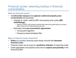
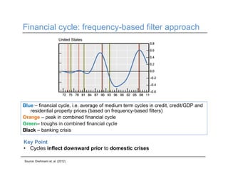
1. Financial Cycles:
What are they and how to compute them?
IMF Area Department Presentation
March 17, 2015
Benjamin Huston
Sanaa Nadeem
Inci Otker-Robe

2. Financial cycles: detecting buildup in financial
vulnerabilities
What are financial cycles?
• A multivariate measure that captures credit and property price
co-movement and periodicity
– Average of credit, credit-to-GDP, and property price cycles (BIS
methodology).
• Sept 2011 GFSR: credit growth combined with asset price growth tends to provide a
better measure of an impending financial crisis.
– Estimated using two econometric approaches:
• Turning point algorithm
• Frequency-based bandpass filter
Why are financial cycles important?
• Peaks of a country’s financial cycle closely coincide with domestic
financial crises
• Financial cycles can be used as a predictive indicator of impending crises
• Credit aggregates and property prices tend to capture procyclicality in the
financial system

3. Financial cycle: elements
Example: United States (Drehmann et. al, 2012)
Key Point
• Crises fall between medium-term peak/trough pairs
• Recessions fall between short-term peak/trough pairs
Source: Drehmann et. al. (2012)

4. Financial cycle: frequency-based filter approach
Blue – financial cycle, i.e. average of medium term cycles in credit, credit/GDP and
residential property prices (based on frequency-based filters)
Orange – peak in combined financial cycle
Green– troughs in combined financial cycle
Black – banking crisis
Source: Drehmann et. al. (2012)
Key Point
• Cycles inflect downward prior to domestic crises

5. Computing financial cycles: data
• Three input series:
– Real residential property prices
– Real credit
– Real credit/real GDP ratio
• Series should be in levels and standardized to a common point in
time (e.g., 2010-Q3)
• Nominal series deflated using either GDP deflator or consumer
inflation rates
• Recommended minimum sample size: 40 years of quarterly data

6. Computing financial cycles: techniques
Turning point analysis
– Identifies local maxima and minima
– Input series are real, normalized levels (as in prior slide)
– Apply Quarterly Bry-Boschan (BBQ) algorithm (Harding, Pagen; 2002) to each
input series
• parameters: min phase of 2 quarters; min cycle length of 40 quarters
– Use Harding and Pagen (2006) algorithm to combine input series’
peaks/troughs and get financial cycle
Frequency-based filter analysis
– Identifies downward inflections in averaged cyclical components
– Convert input series into 4-quarter log-differences
– Apply asymmetric Christiano-Fitzgerald band pass filter (Christiano, Fitzgerald;
2003)
• parameters: min/max periods of 8 and120 quarters; stationarity assumed
• extract cyclical components from each input series
– take simple average of input series’ cyclical components to get financial cycle

7. Stylized facts
• Financial cycles have a lower frequency (10-20 vs. 6-8 years) and
higher amplitude than traditional business cycles
• Recessions that coincide with financial cycle contractions tend to be
deeper.
Source: Drehmann et. al. (2012)
United States

8. Guidance for Low Income Countries
Issue
Lack of long and relevant time series and frequent structural breaks
make computing financial cycles difficult
Recommendations
• Compute Credit/GDP gap (template from Staff Guidance Note on
Macroprudential Policy; FSI-based tools (MCM Financial Toolbox)
• Complement Credit/GDP gap (core indicator) with additional
measures (e.g. real credit growth, credit/GDP level and growth,
structural private sector gap, debt service to income ratio, LTV ratio,
signs of FX and funding mismatches, other market-based indicators)
(Source: Staff Guidance Note: Table 1 in the main paper and Box 1 in
the background paper for Low Income Countries)
• Examine credit and asset price co-movement over shorter time
periods
• Always consider country specific circumstances

9. Credit/GDP gap as a financial cycle proxy
South Africa
Denmark
Financial Cycle Credit/GDP Gap Credit Cycle
Financial Cycle Credit/GDP Gap Credit Cycle
*Financial cycles and credit cycles computed using frequency-based filter approach; red lines mark onset of 2008 financial crisis; credit/GDP gap
calculated using annual credit data that is temporally disaggregated to a quarterly frequency

10. Considerations for Low Income Countries
• Is rapid credit growth a symptom of a buildup in financial stability
risks or financial deepening?
Source: Rapid Credit growth in Central and Eastern Europe: Endless Boom or Early Warning? Eds. Charles Enoch and Inci Ötker-Robe,
Palgrave MacMillan (March 2007).

11. Considerations for Low Income Countries (Cont’d)
• Are house price increases the most accurate characterization
of rising financial stability risks for LICs (vs. household
indebtedness, household consumption, corporate leverage,
government deficit, volatile capital flows, export
concentration)
• Combine information from other potential contributors: e.g.
tax policy, supply constraints, credit from nonbank sector
• Compare recent indicators with a relevant peer group if
sample is too short

12. References
• Borio, C. (2012). The financial cycle and macroeconomics: What have we
learnt? BIS Working Paper No. 395.
• Christiano, L. and Fitzgerald T.J. (2003). The bandpass filter. International
Economic Review, 44(2):435- 65.Claessens, S., Kose, A. and Terrones, M.
(2011) Financial Cycles: What? How? When? IMF Working Paper 11/76
• Drehmann, M, Borio, C., and Tsatsaronis, K. (2012). Characterizing the financial
cycle: don’t lose sight of the medium term! BIS Working Paper No. 380.
• Harding, D. and Pagan A. (2002). Dissecting the Cycle: A Methodological
Investigation. Journal of Monetary Economics 49 (2), 365–381
• ---. (2006). Synchronization of cycles, Journal of Econometrics, 132, 59-79.
• IMF 2014. Staff Guidance Note on Macroprudential Policy.
• ---. Staff Guidance Note on Macroprudential Policy. Detailed Guidance
• ---. Staff Guidance Note on Macroprudential Policy Considerations for Low
Income Countries. IMF Policy Paper.