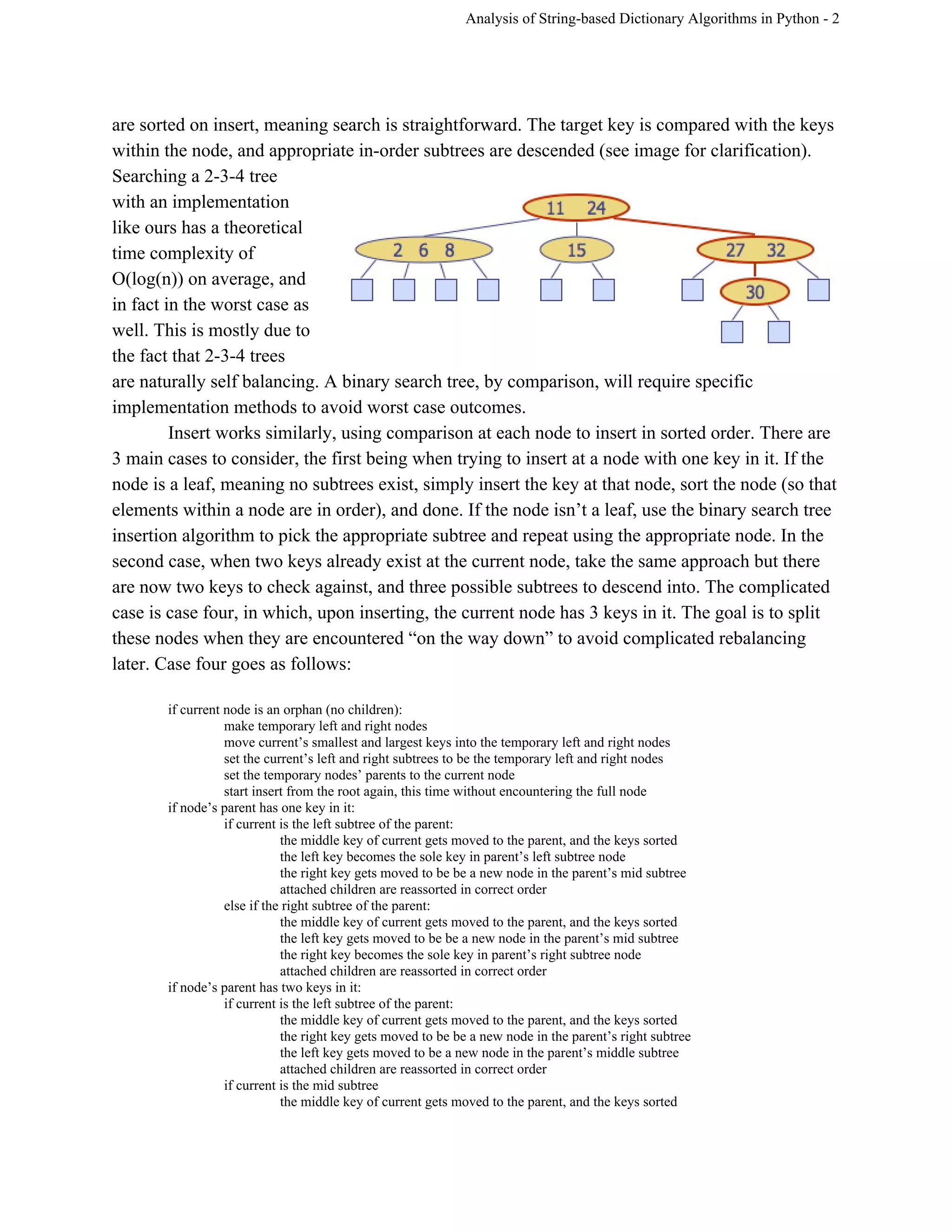
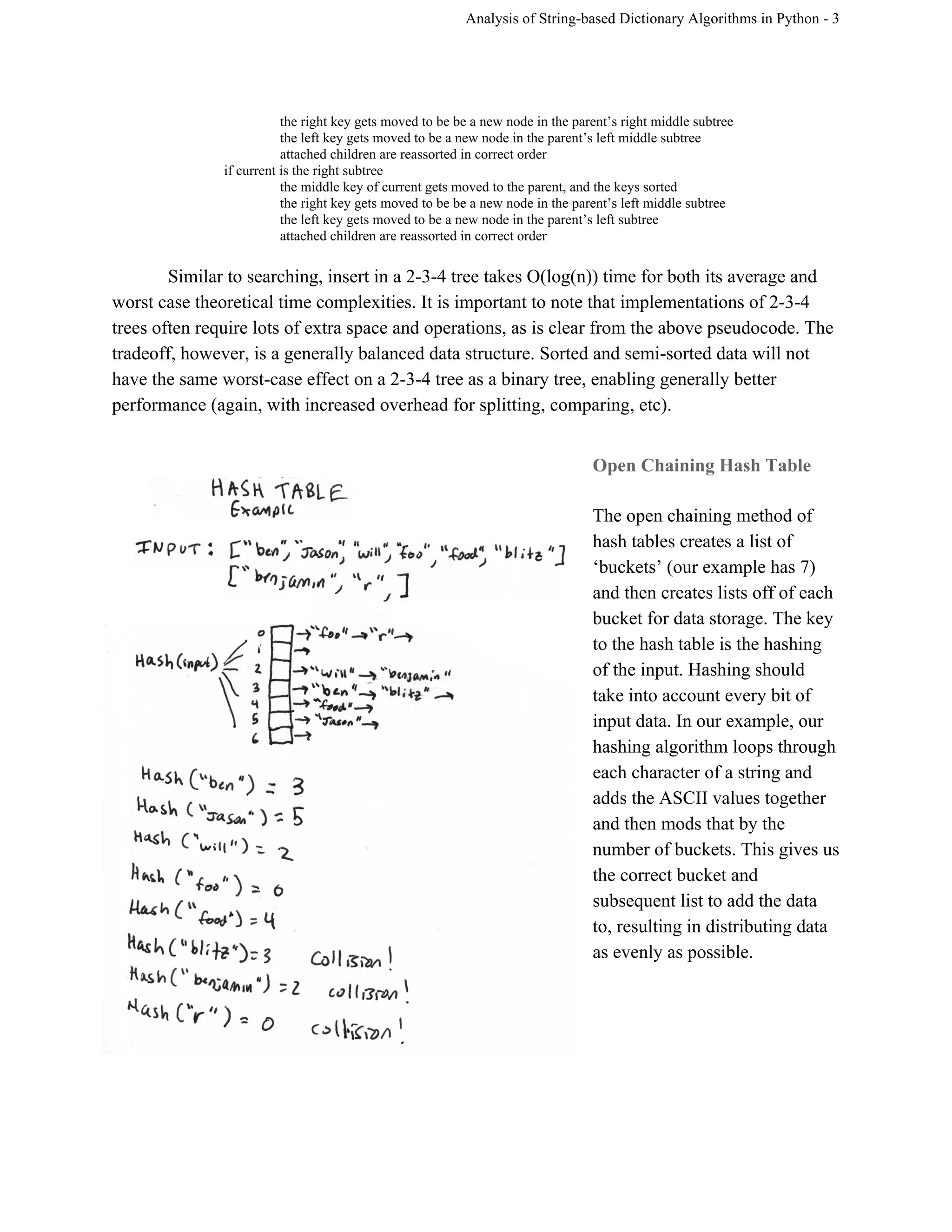
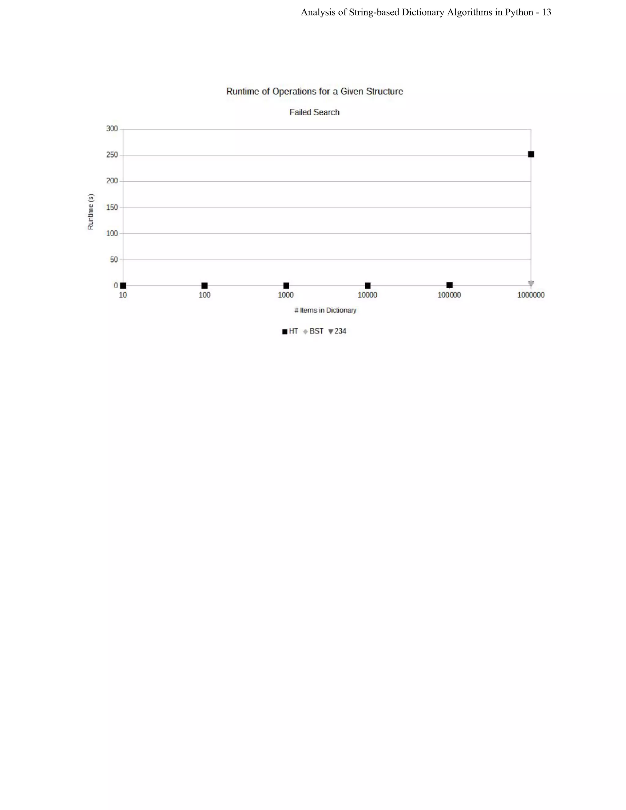
This document analyzes the implementations and efficiencies of three Python dictionary algorithms: an open-hashing table, binary search tree (BST), and 2-3-4 tree. The group implemented each data structure and tested their performance. The BST has insertion and selection times of O(log n) on average and O(n) worst-case. The 2-3-4 tree also has O(log n) average and worst-case times for insertion and searching due to self-balancing, though it requires more space. The open-hashing table uses hashing to distribute keys across buckets, but collisions degrade performance with many elements. The group encountered challenges with Python concepts like null values but overcame them through research

1.
Ben Reichert
Jason Hannan
Will Oberfest
Analysis of String­based Dictionary Algorithms in Python
Project purpose
To thoroughly understand the implementations and efficiencies of string­based dictionary
implementations written in Python. We chose three implementation algorithms of dictionaries:
an open­hashing table, binary­search tree, and 2­3­4 tree.
Chosen Algorithm Descriptions
Binary Search Tree
Binary Search Tree is a simple program to understand and implement. This is a trivial
topic that every second year or higher C.S. major comes to understand, therefore I will not cover
the details of how to build a BST. The algorithmic complexity of Insertion and Selection from a
BST are relatively similar. Insertion is not tightly bound. Its worst case is when the data is
inserted in order or reverse order. This builds a Linear Linked List and has O(n) for Insertion. In
the best case scenario you will get Θ(Log n). This is because the data gets distributed evenly
across the tree and our height will be Log n.
For Selection we have a best case scenario of Θ(1) being that the item we are looking for
is the first element of the tree. Worst case scenario is when either its the last element of the tree,
and the tree is a linear linked list, or when the item isn’t contained within the tree at all. This
gives us O(n) for Selection.
Key piece of information to know when counting the complexity of a BST is that your
basic operation is anytime you have to traverse the tree. This always happens on a recursive call
of one of its children. See attached sheet for algorithm complexity calculations.
2­3­4 Tree
Search and traversal in a 2­3­4 tree work similarly to a binary search tree, except that
each node can hold multiple keys. For our implementation, each node is comprised of an object
meant to hold three keys, as well as 4 objects with pointers to children, and a final pointer to a
parent. The four children represent subtrees; a left, left­middle, right­middle, and right. At any
given time, a node in a 2­3­4 tree will have either one, two, or three keys within the current node.
If one key exists, the tree has a left and right subtree. If two keys exist, a left, middle, and right
subtree exist. When three keys exist, there are left, left middle, right middle, and right subtrees.
Searching a 2­3­4 tree is relatively straightforward. It works similarly to a binary search
tree, but with additional comparisons at each node before descending deeper into the tree. Nodes

2. Analysis of String­based Dictionary Algorithms in Python ­ 2
are sorted on insert, meaning search is straightforward. The target key is compared with the keys
within the node, and appropriate in­order subtrees are descended (see image for clarification).
Searching a 2­3­4 tree
with an implementation
like ours has a theoretical
time complexity of
O(log(n)) on average, and
in fact in the worst case as
well. This is mostly due to
the fact that 2­3­4 trees
are naturally self balancing. A binary search tree, by comparison, will require specific
implementation methods to avoid worst case outcomes.
Insert works similarly, using comparison at each node to insert in sorted order. There are
3 main cases to consider, the first being when trying to insert at a node with one key in it. If the
node is a leaf, meaning no subtrees exist, simply insert the key at that node, sort the node (so that
elements within a node are in order), and done. If the node isn’t a leaf, use the binary search tree
insertion algorithm to pick the appropriate subtree and repeat using the appropriate node. In the
second case, when two keys already exist at the current node, take the same approach but there
are now two keys to check against, and three possible subtrees to descend into. The complicated
case is case four, in which, upon inserting, the current node has 3 keys in it. The goal is to split
these nodes when they are encountered “on the way down” to avoid complicated rebalancing
later. Case four goes as follows:
if current node is an orphan (no children):
make temporary left and right nodes
move current’s smallest and largest keys into the temporary left and right nodes
set the current’s left and right subtrees to be the temporary left and right nodes
set the temporary nodes’ parents to the current node
start insert from the root again, this time without encountering the full node
if node’s parent has one key in it:
if current is the left subtree of the parent:
the middle key of current gets moved to the parent, and the keys sorted
the left key becomes the sole key in parent’s left subtree node
the right key gets moved to be be a new node in the parent’s mid subtree
attached children are reassorted in correct order
else if the right subtree of the parent:
the middle key of current gets moved to the parent, and the keys sorted
the left key gets moved to be be a new node in the parent’s mid subtree
the right key becomes the sole key in parent’s right subtree node
attached children are reassorted in correct order
if node’s parent has two keys in it:
if current is the left subtree of the parent:
the middle key of current gets moved to the parent, and the keys sorted
the right key gets moved to be be a new node in the parent’s right subtree
the left key gets moved to be a new node in the parent’s middle subtree
attached children are reassorted in correct order
if current is the mid subtree
the middle key of current gets moved to the parent, and the keys sorted

3. Analysis of String­based Dictionary Algorithms in Python ­ 3
the right key gets moved to be be a new node in the parent’s right middle subtree
the left key gets moved to be a new node in the parent’s left middle subtree
attached children are reassorted in correct order
if current is the right subtree
the middle key of current gets moved to the parent, and the keys sorted
the right key gets moved to be be a new node in the parent’s left middle subtree
the left key gets moved to be a new node in the parent’s left subtree
attached children are reassorted in correct order
Similar to searching, insert in a 2­3­4 tree takes O(log(n)) time for both its average and
worst case theoretical time complexities. It is important to note that implementations of 2­3­4
trees often require lots of extra space and operations, as is clear from the above pseudocode. The
tradeoff, however, is a generally balanced data structure. Sorted and semi­sorted data will not
have the same worst­case effect on a 2­3­4 tree as a binary tree, enabling generally better
performance (again, with increased overhead for splitting, comparing, etc).
Open Chaining Hash Table
The open chaining method of
hash tables creates a list of
‘buckets’ (our example has 7)
and then creates lists off of each
bucket for data storage. The key
to the hash table is the hashing
of the input. Hashing should
take into account every bit of
input data. In our example, our
hashing algorithm loops through
each character of a string and
adds the ASCII values together
and then mods that by the
number of buckets. This gives us
the correct bucket and
subsequent list to add the data
to, resulting in distributing data
as evenly as possible.

4. Analysis of String­based Dictionary Algorithms in Python ­ 4
Code snippets in Python
Hash Table
Hashing algorithm hash function.
Hash table search code.
BST
BST insertion code.

5. Analysis of String­based Dictionary Algorithms in Python ­ 5
BST search code.
2­3­4 Tree
Very small section of the 2­3­4 tree insert algorithm. Many other cases are in the full source
available on Github (see link in conclusion).
Python Implementation
Because each data structure was implemented by a different team member, different
issues with the language of choice arose for different members. For instance, Ben had no
experience writing testing systems, or generating random strings for this project. While this was
new, stackoverflow and forums helped guide our group in the right direction. We were able to
create a very solid testing framework from scratch. Jason didn’t have too many problems with

6. Analysis of String­based Dictionary Algorithms in Python ­ 6
the BST implementation, but returning values as tuples and lists was new to him. Will had
almost zero experience writing in python, so the majority of the syntax required extra attention
and learning.
Our Hash table used a static size of 57 list bucket elements. This obviously causes
problems with millions of elements and tons of collisions, but for the sake of complexity analysis
we did not want to change the table elements as we thought it may affect our complexity and
running time analysis.
There were things with Python that we did not expect, but learned from and dealt with
properly. Having a background in C++, the concept of Null not being the same in Python, as well
as not having pointers in the first place, led to needing some unique solutions. We did not expect
that a majority of the time of running tests was actually generating the pseudo­random strings,
and not actually running the algorithms. We also found out that we could not reasonably generate
sets of strings over 10 million elements without running into gigs of generated input data and
massive running times for the algorithms. Ben’s hash table implementation would take over an
hour per trial, and it had 30 to do per test at 100 million elements. Because of this we reduced
our max set to 1,000,000 strings. We can not comment on the specific details of Python’s list and
other object memory space, we do know that the overhead of these types of objects is roughly 4x
that of the original data. This could lead to what we like to refer to as “Python bloating”. With
this in mind, our choice of Python was a solid one as it allowed us to get moving quickly and
effectively, but may not be the most efficient for these algorithms.
Since our code was single­threaded, it took a long time to run all the tests. While we may
have been able to test multiple algorithms in parallel, we did not want to bother with the added
complexity, headaches, and unreliability.

7. Analysis of String­based Dictionary Algorithms in Python ­ 7
Single core Python testing suite running. Generating strings may have been faster with
threading as well as testing multiple algorithms in parallel (but that is outside the scope of
this project).
Testing
Our testing suite is where most of our originality stems from. It was written from the
ground up for this specific project in mind, and therefore was tailored to fit our needs as best
possible. We start out by generating random strings as input. These strings are uppercase ASCII
of length 9. For example: ‘TGHAJDLDJ’. Code for string generation follows:

8. Analysis of String­based Dictionary Algorithms in Python ­ 8
Class used for generating random strings for testing.
We wrote a Worker class that handled the creation of lists of random strings. It would also pick a
subset of strings in the random list used for searching. It would also generate more random
strings that were guaranteed ​not​ to be in the valid search strings, so we could purposely check for
worst case running time. Each set of strings was generate at runtime of that specific instance of
the test and run through each algorithm for comparison. We picked random string counts of 10,
100, 1000, 10000, 100000, 1000000 for testing.
For the actual runtime time checking, we used a basic, but reliable system for
measurement. We would run insertion, search, and then invalid search for every algorithm with
10 trials each for a more reliable statistical average. Right before each trial run we would record
the current system time using Python’s built in time library, and the end time after the test. The
difference between start and end time was the running time. We also kept track of each trial’s
basic operation count.
We create the tester such that it would log results automatically to CSV formatted files
for later graphs and analysis. We also stored the input strings as a Python ‘pickled’ object to disk
for later reference. The true beauty of the tester was that we could run a new series of tests with a
single command, and come back later to fetch data without any other interaction.
To test the correctness of our algorithms we inserted all strings into the implementation,
and then searched for each one. If we found every string, we could assume that the
implementation stores and searches for strings properly (which they did!). On the same page, we
also made sure that none of the invalid strings were found in each algorithm. We did this to
ensure our implementations were correctly storing data and not storing data that ​shouldn’t ​be
there. Ben had a great time writing the testing suite and all the automation components of it to
ensure a easy, reliable method of testing our implementations.

9. Analysis of String­based Dictionary Algorithms in Python ­ 9
Algorithm Complexity
The time­complexity for Insert and Search on average is O(log n). For search this is
shown through our trials. We can see that it was exactly what it was suppose to be. It shows that
for 10 items it took 4 basic operations to find the data and return it. This is the ceiling of log n.
This shows not only was the time­complexity nearly on the spot, that the code implementation
was correctly counting the basic operations and that it was a near balanced tree. The data for
Insert is a little more complex because it is the summation of inserts. when looking at the table
for 10 items. It shows that all runs took 36 basic operations to insert all data. This is roughly the
cost of of the summation of 10 inserts when the insert complexity is log n. This shows that our
insertion is fairly random and that it is building a nearly balanced tree. This leads back to
showing a fundamentally sound counting of basic operations and coding of a binary search tree.
Similarly, we know 2­3­4 trees have the same time complexity for search as BST’s on
average, O(log n). It’s easy to see in the tables for number of operations that the 2­3­4 tree
performs similarly to BST’s, although it does deviate from being strictly equal. This is likely in
part due to implementation, but it is clear from the data that they perform similarly given the
scale of the data. In addition, we know 2­3­4’s also insert in O(log(n)). In terms of number of
operations, 2­3­4’s perform similarly to BST’s once again, although for smaller inputs (under
1000 insertions in our case), the 2­3­4 took significantly fewer operations (roughly half that of
BST’s). This is because of the overhead from splitting while inserting; our counting
implementation for number of operations is related to numbers of comparisons, not creating new
objects, assigning values, etc.
To make that last point explicit, see the run times for our search and insert in both 2­3­4
and BST. The times should match, just as the number of operations did. However, we can see
that the runtime for searches is the only similar part, and matches asymptotic estimates.
However, the insert function, which should also be identical, is far from it. Here we see the
effects of a 2­3­4 tree’s overhead. Insert takes almost twice as long with any decently large
dataset (100 items or more, though by then the gap is quite large). This reinforces the well
established fact that frequent inserts with large numbers of items can become slow in a 2­3­4
tree; that said, if the inserts are infrequent, the results of searching can edge out even a BST in
terms of speed.
The Hash Table basic operation was based on the hashing ops, which are 9 operations
due to the length of strings being 9 characters. The problem we saw immediately, is that the
basic operations were far abstracted from the real running time culprit ­­ searching through the
bucket lists for elements and insertion. The hash table’s average search time is O(1) which would
be the case should there be no collisions. Also, the worst case search time is if the hash table is
built with all elements colliding in the same bucket, resulting in O(n). We found that based on
the random input strings, the elements of the table were fairly evenly distributed. Based on our
recorded data, we noticed that as the hash table grew very large, and the chains as well, the

10. Analysis of String­based Dictionary Algorithms in Python ­ 10
algorithm running time suffered roughly 30x slower than the other two tested. Something else
worth noting is that our hash table implementation appended to the end of a list when adding
data without accessing any list elements. This is what we called “cheating” and if implemented
as a linear linked list, would require traversal of each node and would therefore bring the
insertion time down tremendously. This is why the hash table appears to be roughly 50x faster
than the other algorithms for insertion.
Even though the search of a hash table is O(1), it quickly falls behind the tree algorithms
of O(log(n)) with any reasonably sized data set. This is due to the organizational structure of the
trees compared to the hash table. The hash table cannot change its dimensions while running,
while the trees, to a degree, can shape data flow much more effectively during run­time. This is
one example of why one cannot simply look at the asymptotic complexity and make conclusions
about performance. Also something to consider is that each implementation has a best use case
and knowing when to use which one is just as important as the efficiency of these algorithms.
Conclusions
Due to the high leveled nature of Python we found out that it is very difficult to get the
actual byte usage of an object at any given time. Compounded with this, and the lack of time, we
decided we would not be able to test space and time tradeoffs for this analysis, as much as we
would have liked to.
One of the most notable curiosities of this assignment and dealing with python is that
choosing basic operation to count is tricky. This was particularly clear in the hash function when
from a coding standpoint the innermost loop was on building the key for the input. This was not
even close to being the most expensive operation. Most expensive operation is where we append
items to the end of the hash bucket. This looks from a coding standpoint as just 1 operation but it
is by far the most expensive, in time and space complexities.
When we look at the runtime cost of a 234 tree we will notice that it is expensive. It has
to constantly compare, split and reattach nodes to maintain its balanced form. We noticed it is
roughly 2 times the runtime as a BST. When considering how this performs, if you have a
program that inserts a lot you will probably not want to use a 234 tree due to its performance.
Another thing to note is that 234 tree’s splits can become fairly complex to get right. If you were
to implement this tree in its entirety, the delete and splitting portions will be incredibly complex
and time consuming to code unless someone is incredibly experienced with the cases and how
the splits work. If you were on a time crunch and wanted a data structure that was quick to
implement, the 234 tree would not be recommended for such a task.
For further reference, please see our data and code in our open source GitHub repo at
https://github.com/benjipdx/cs350­project
Sources:

11. Analysis of String­based Dictionary Algorithms in Python ­ 11
http://www2.hawaii.edu/~suthers/courses/ics311s14/Notes/Topic­11.html​ (2­3­4 Image)

12. Analysis of String­based Dictionary Algorithms in Python ­ 12

13. Analysis of String­based Dictionary Algorithms in Python ­ 13