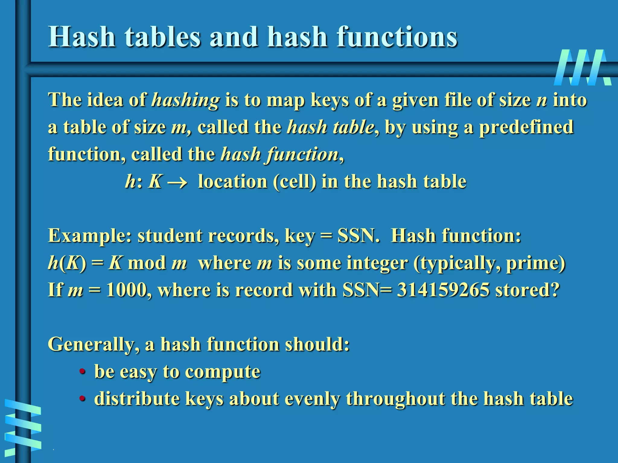
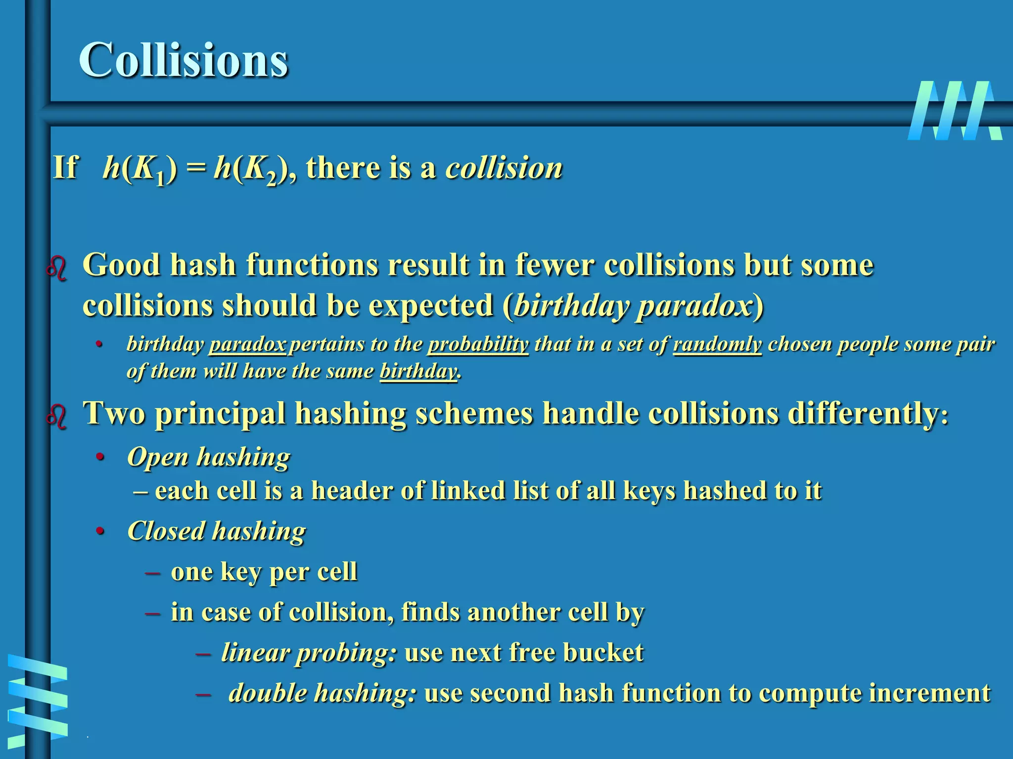
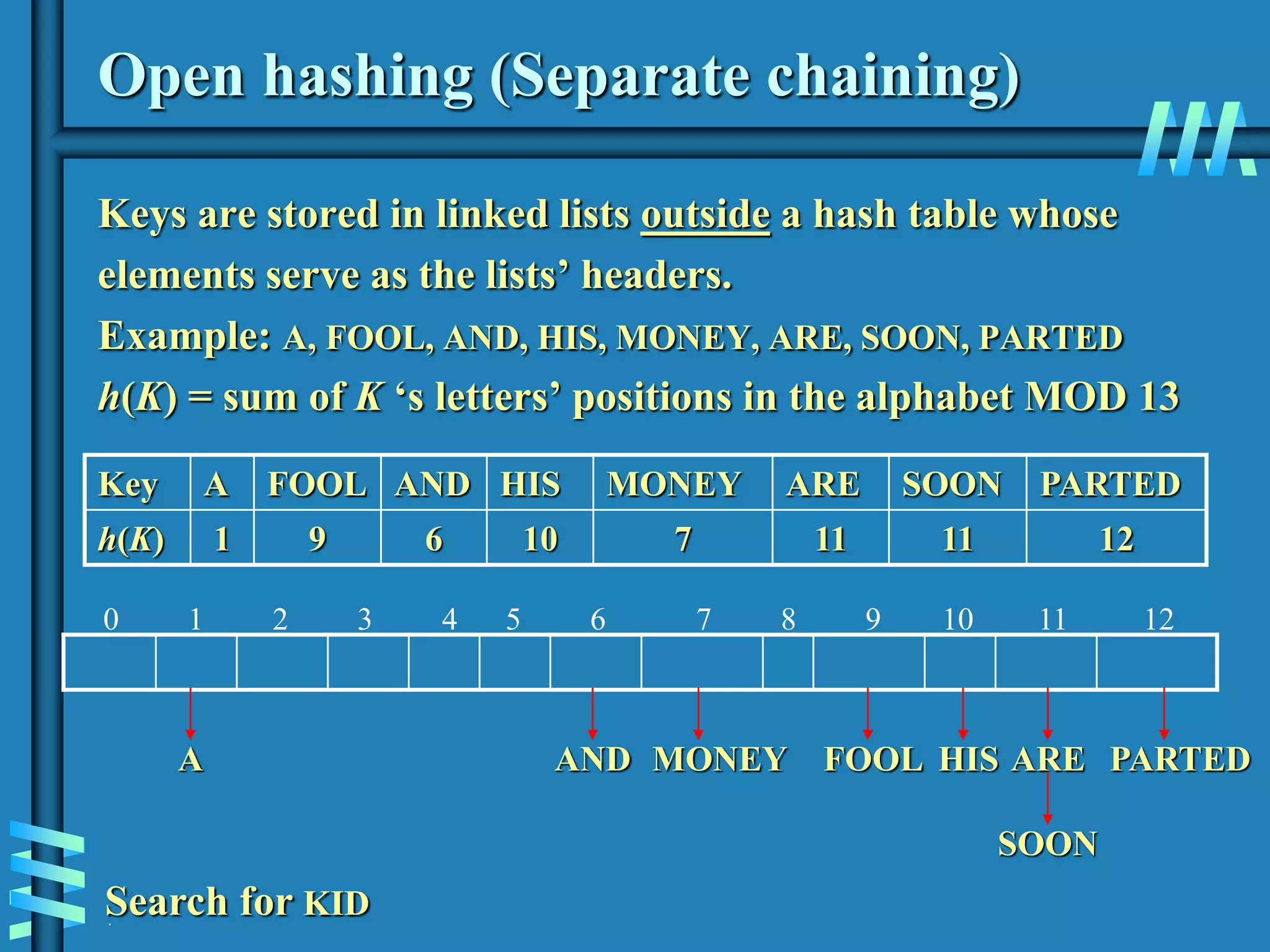
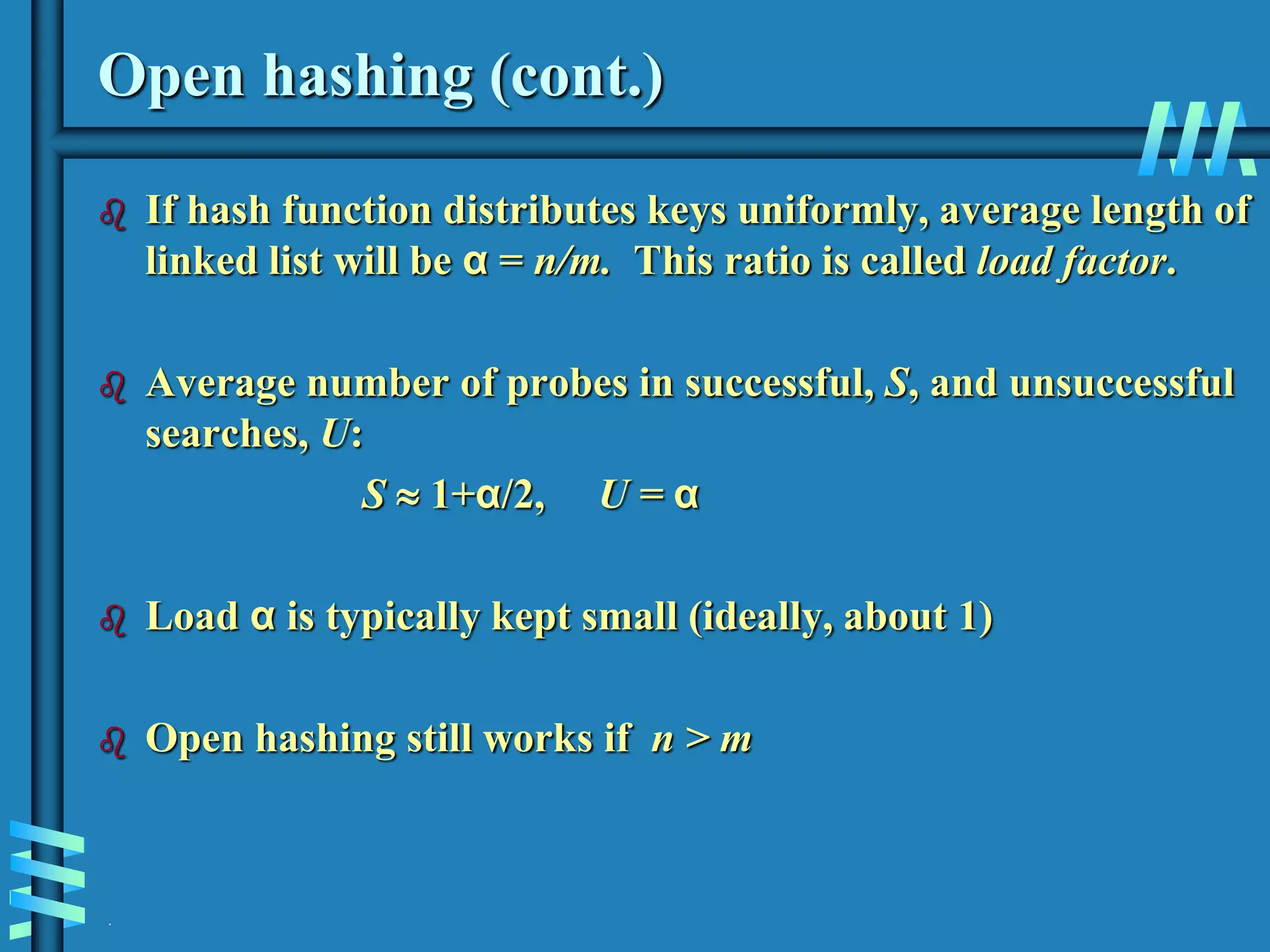
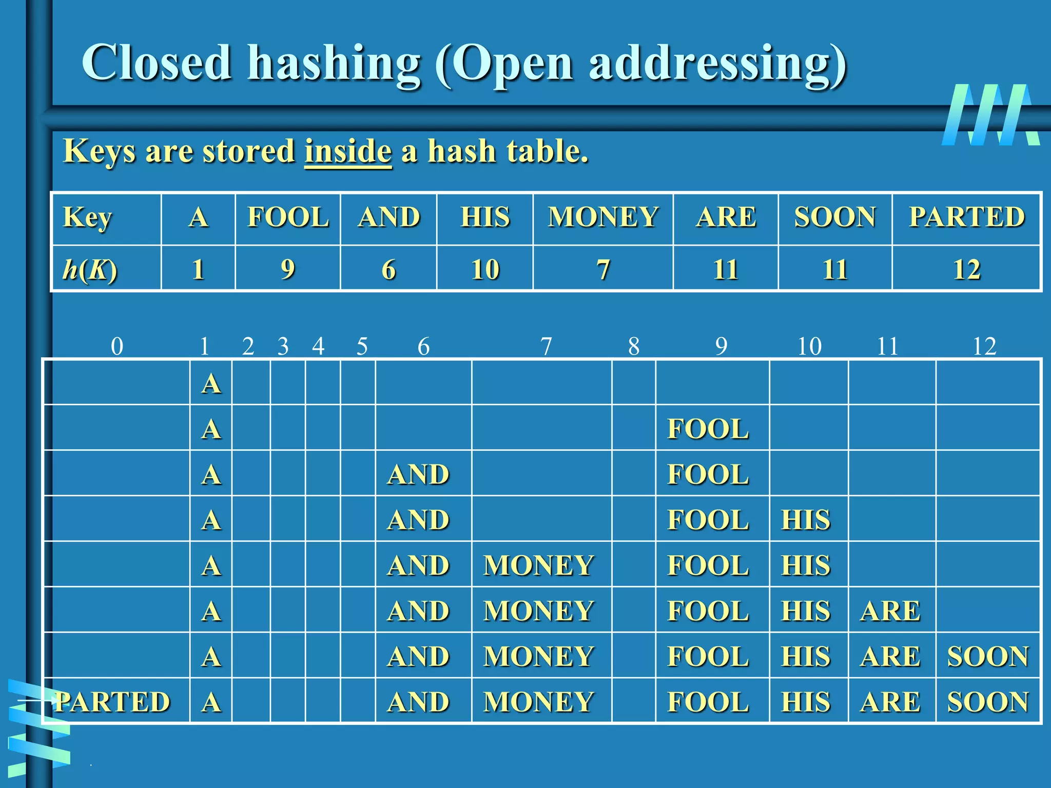
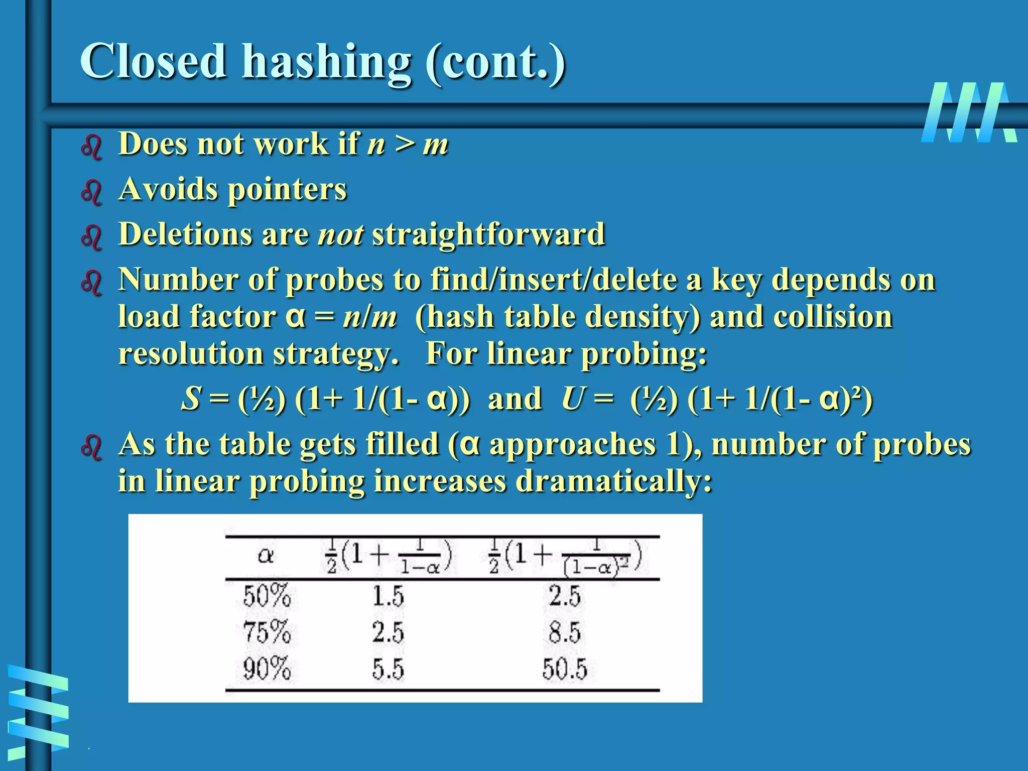
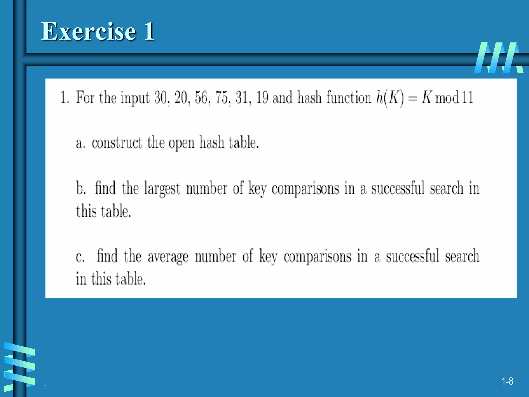
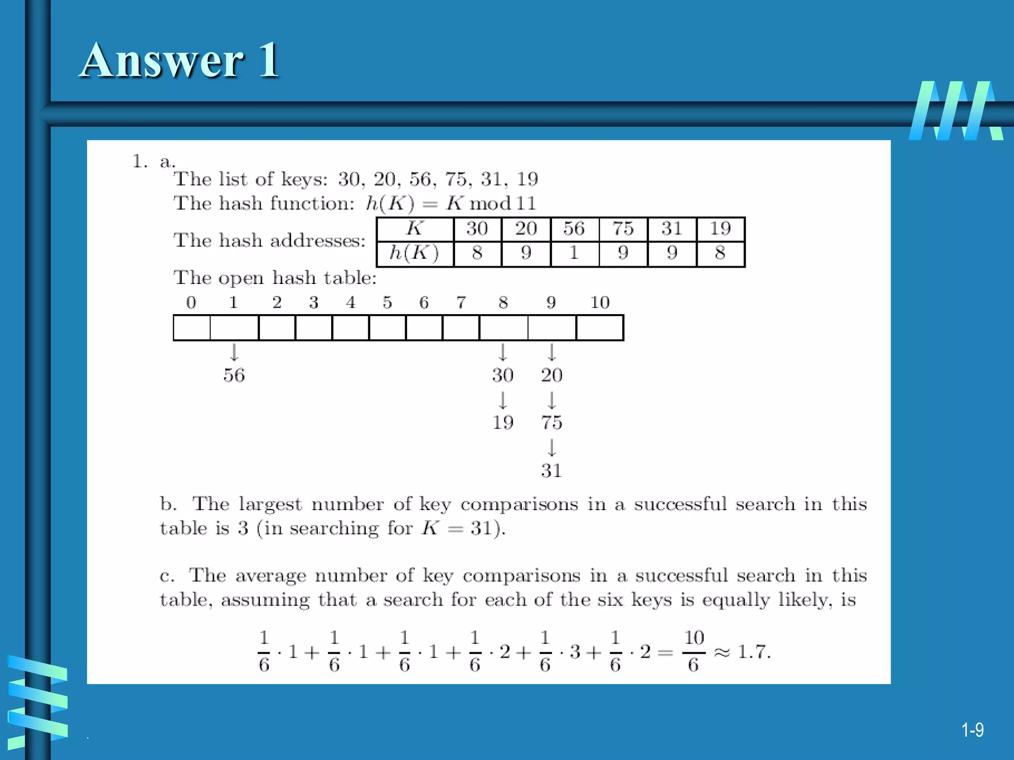
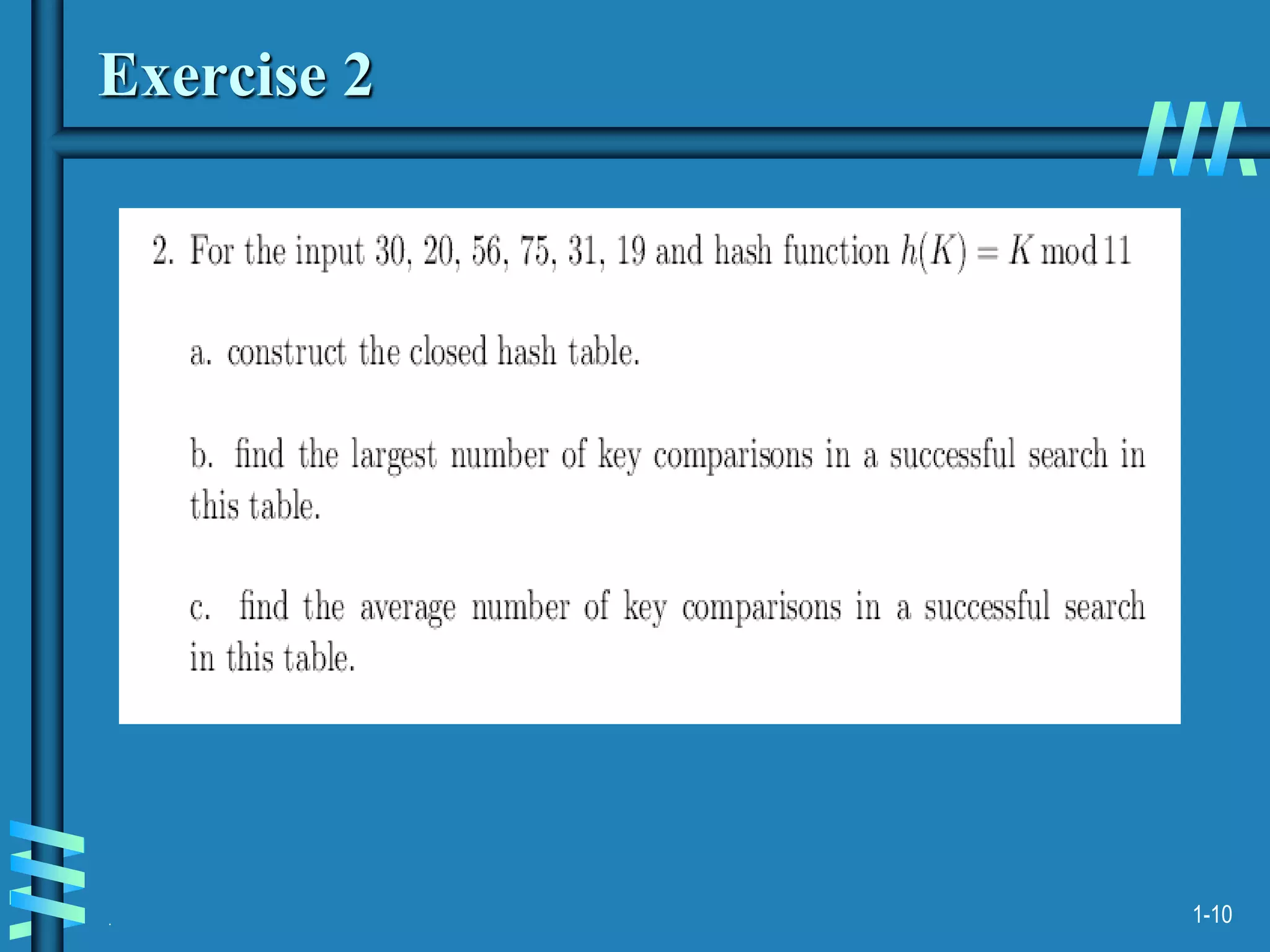
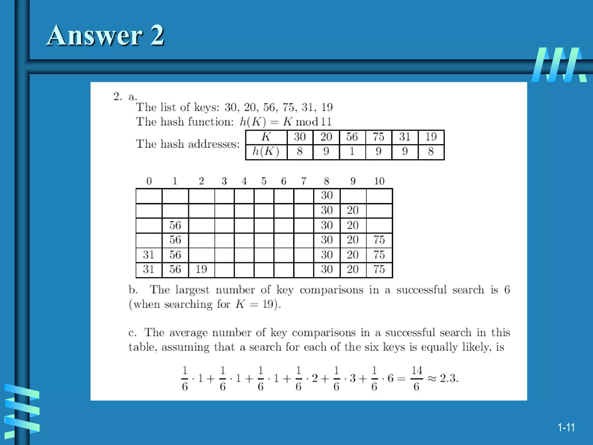
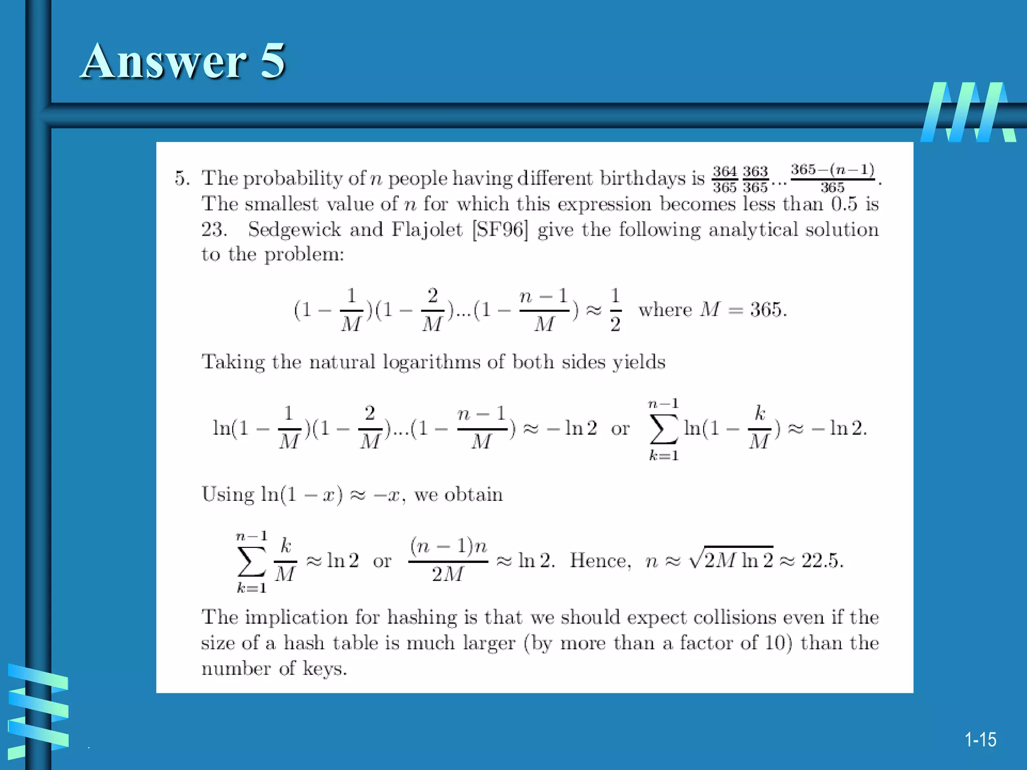
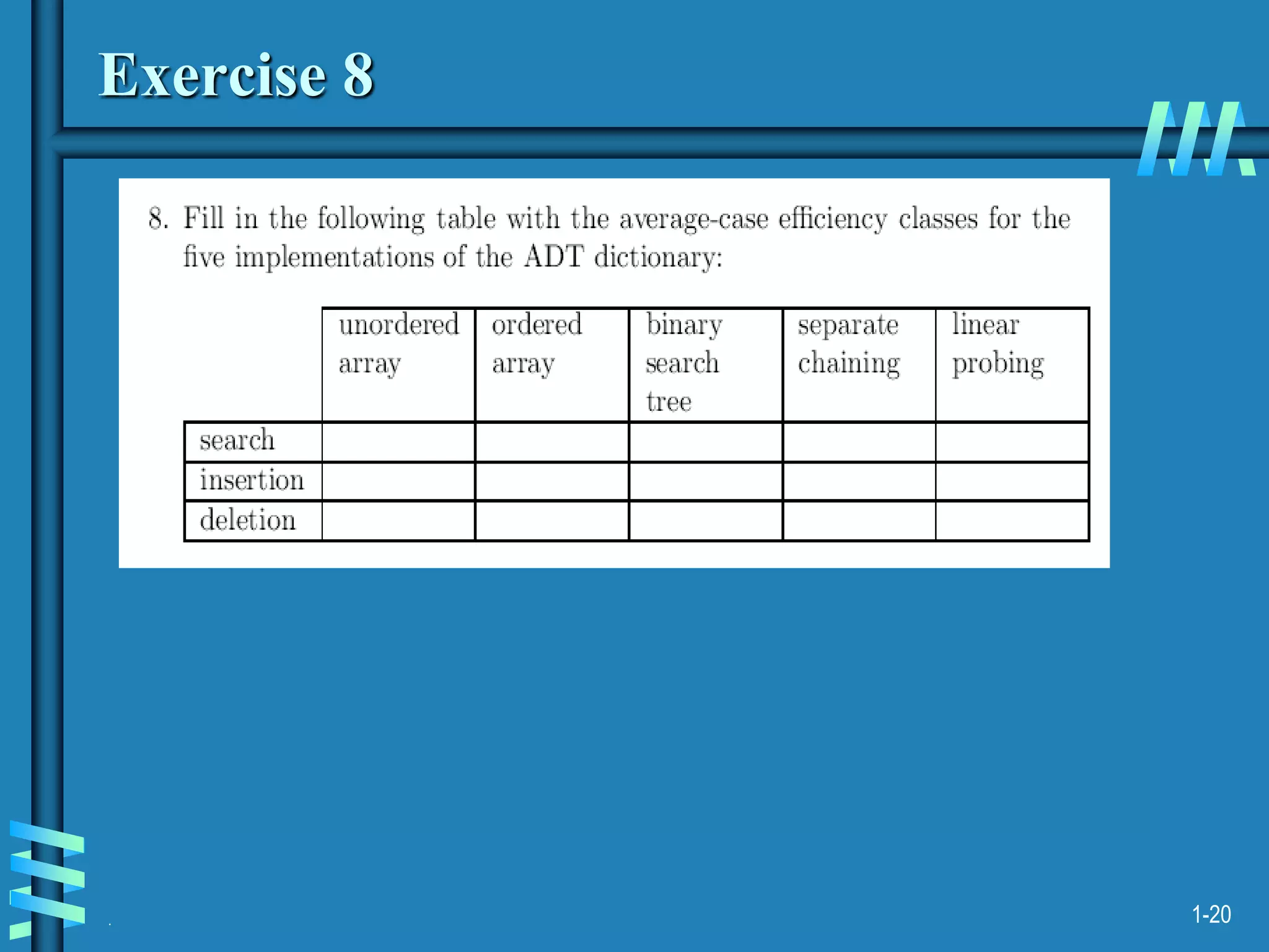
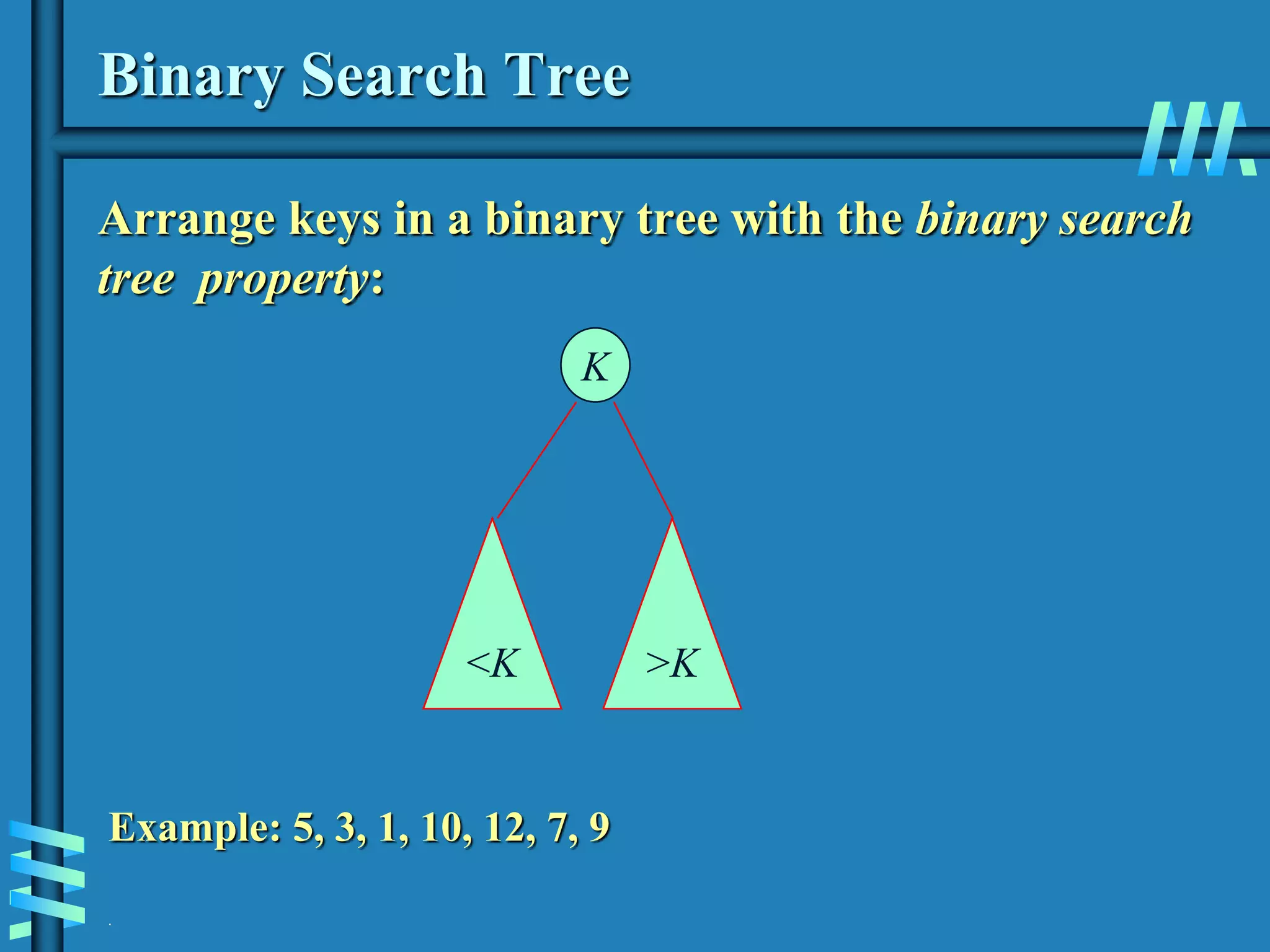
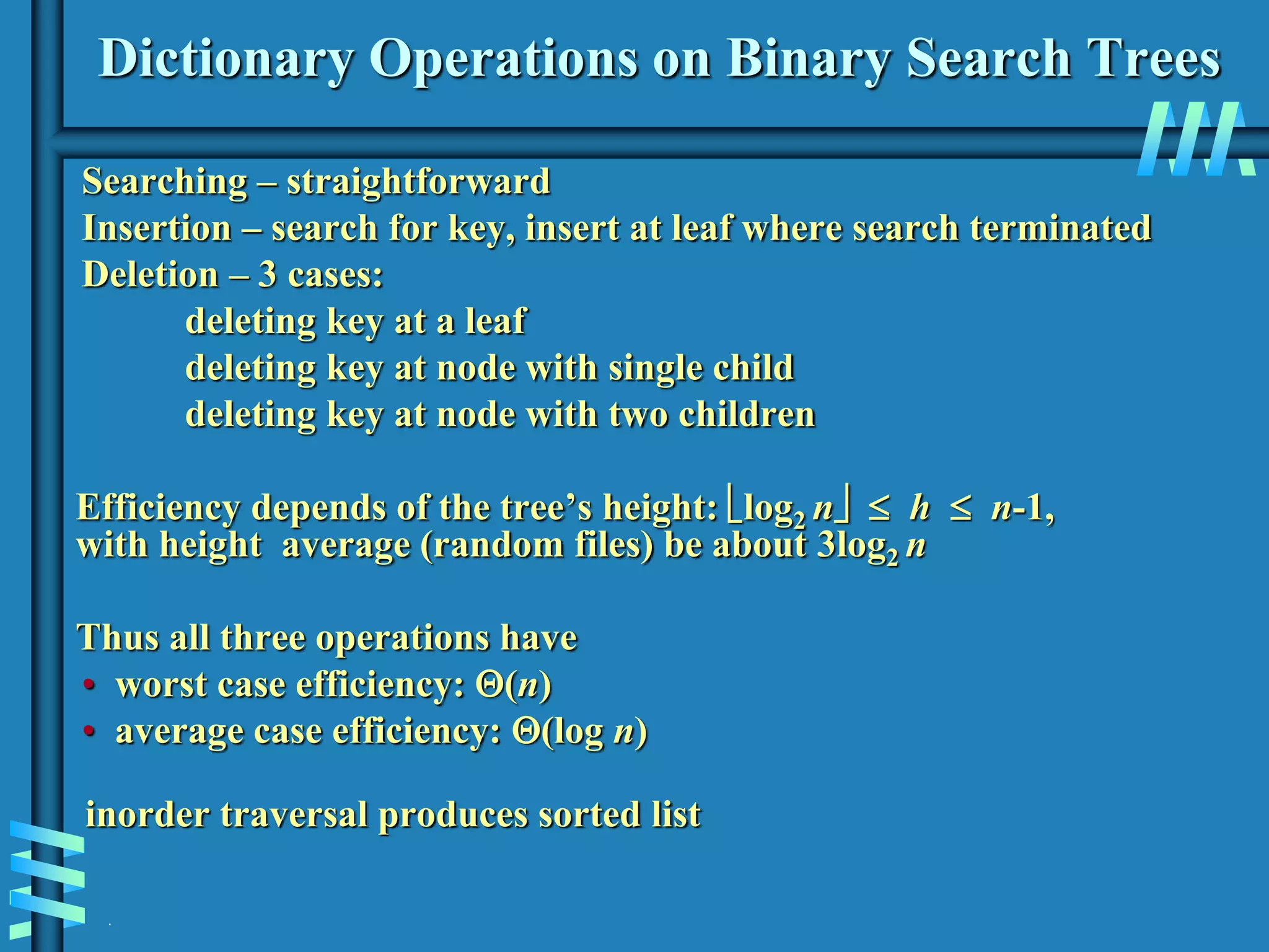
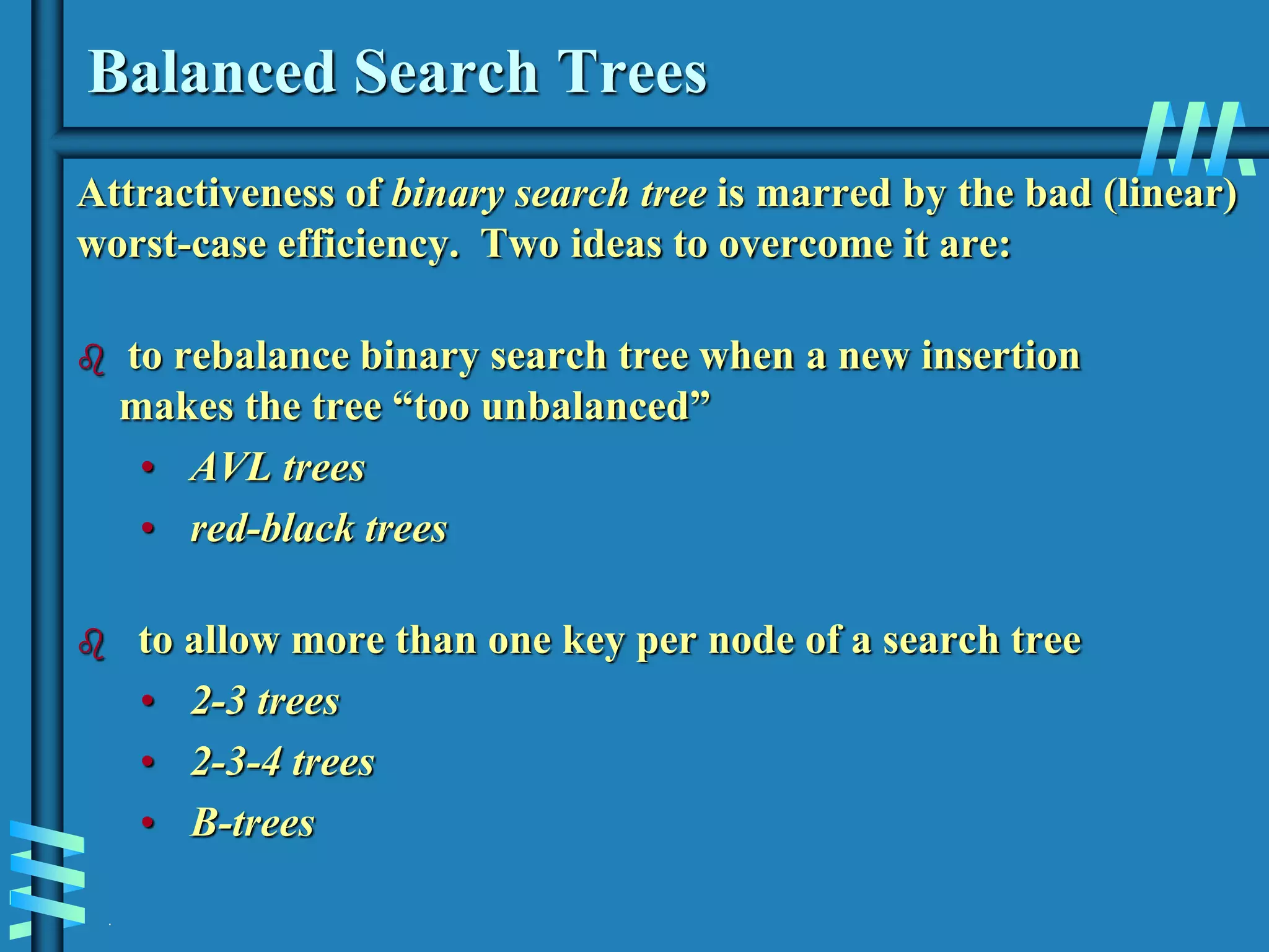
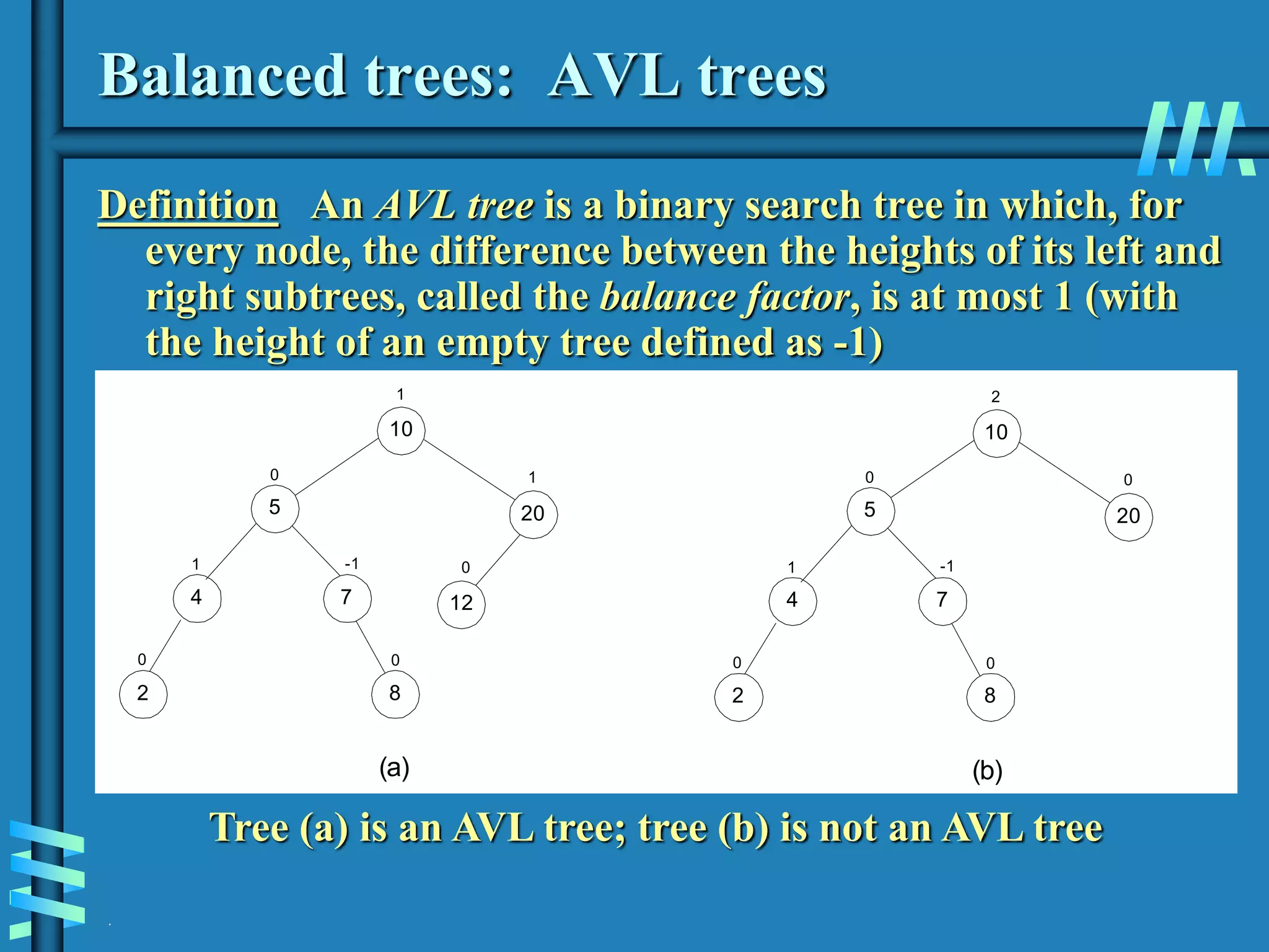
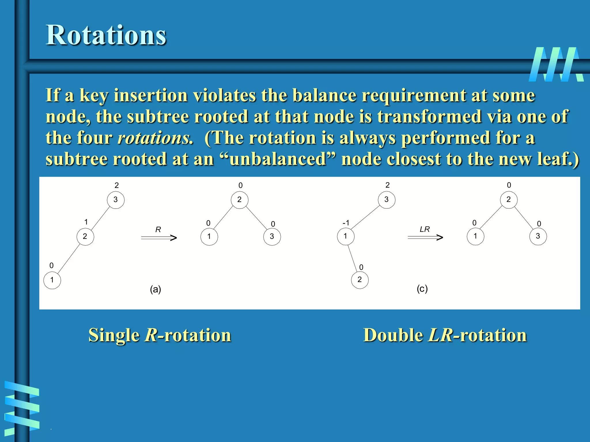
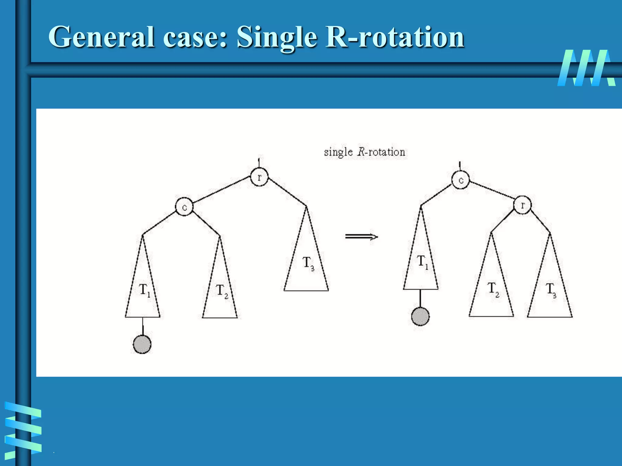
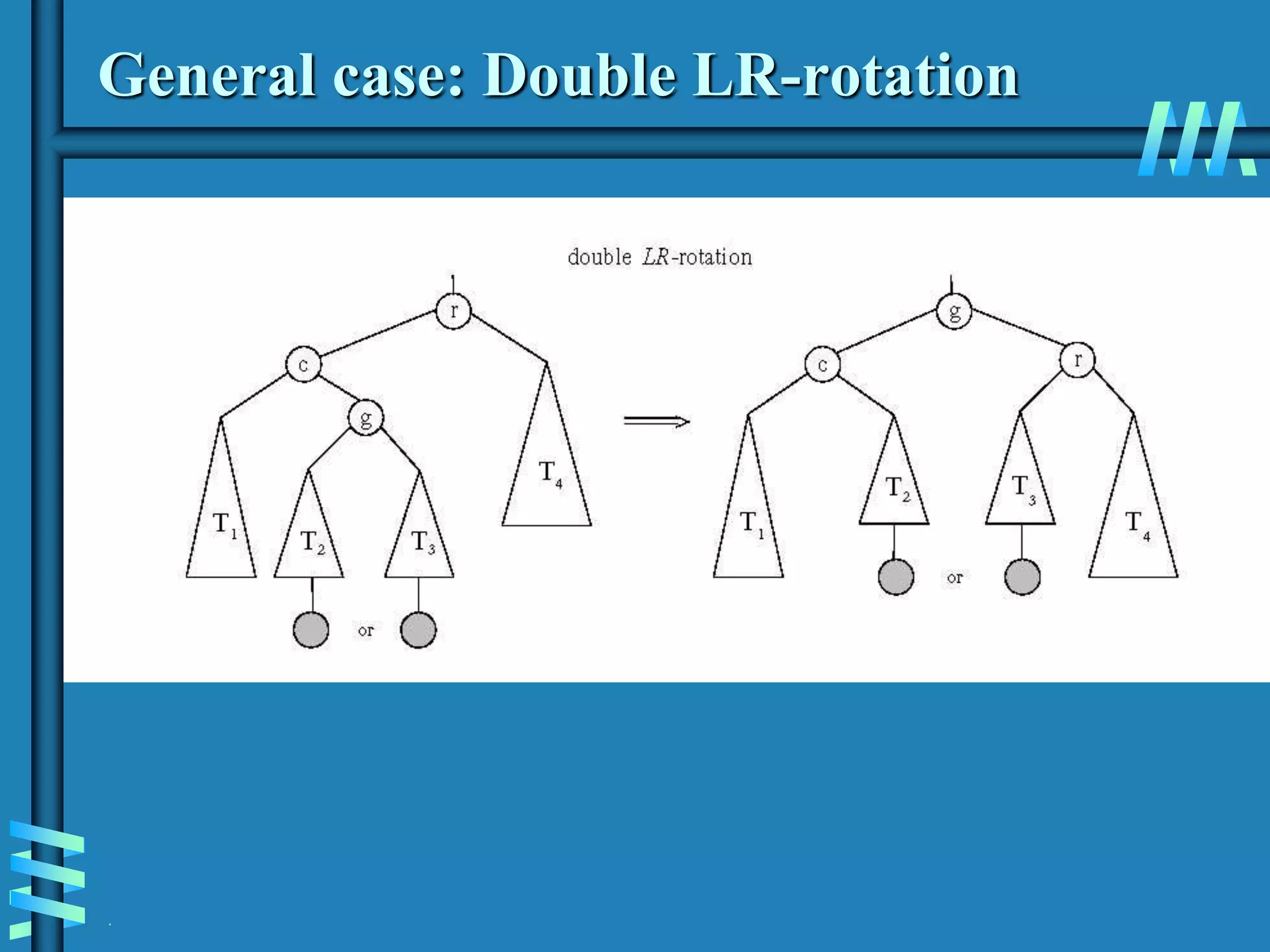
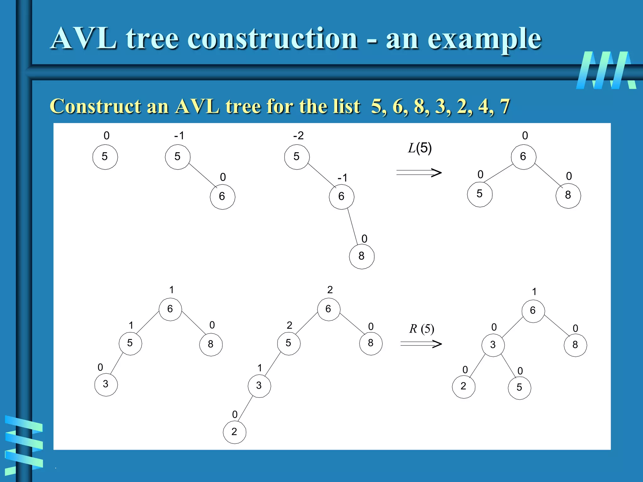
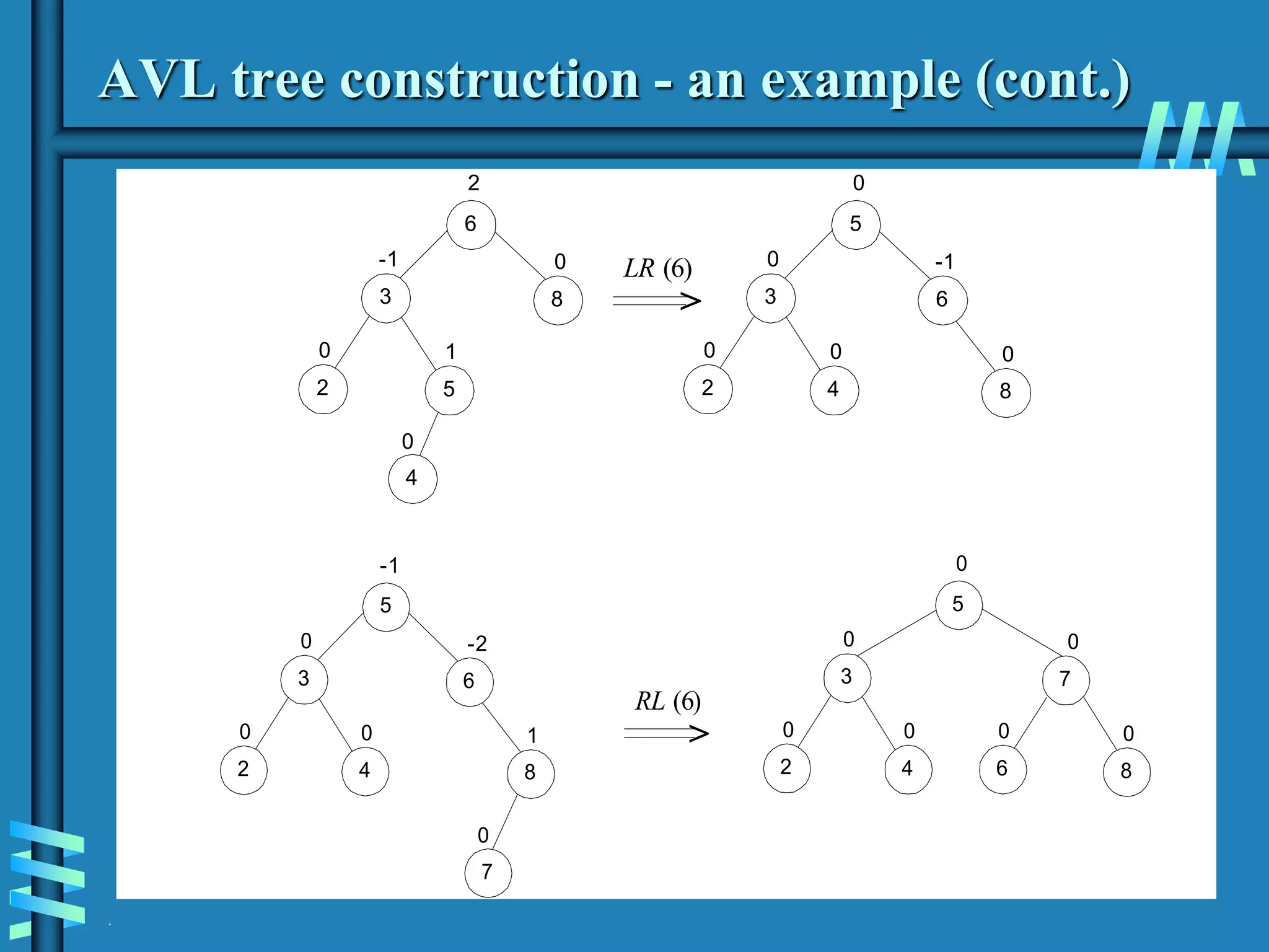
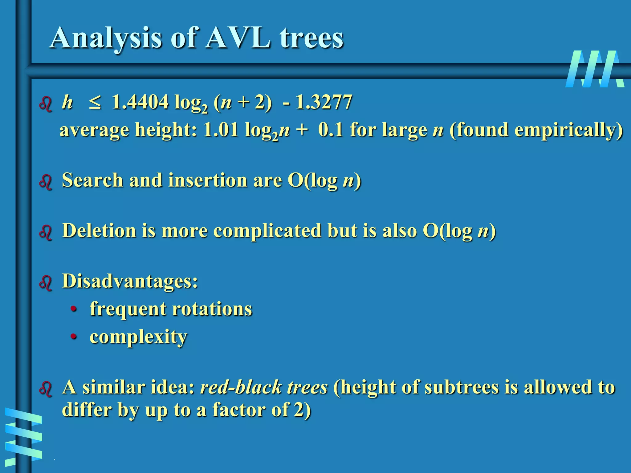
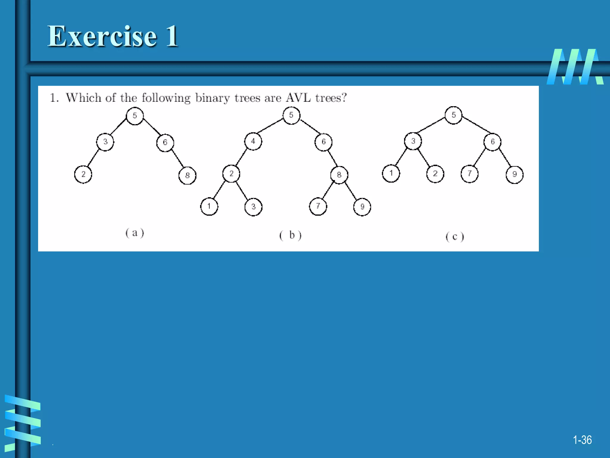
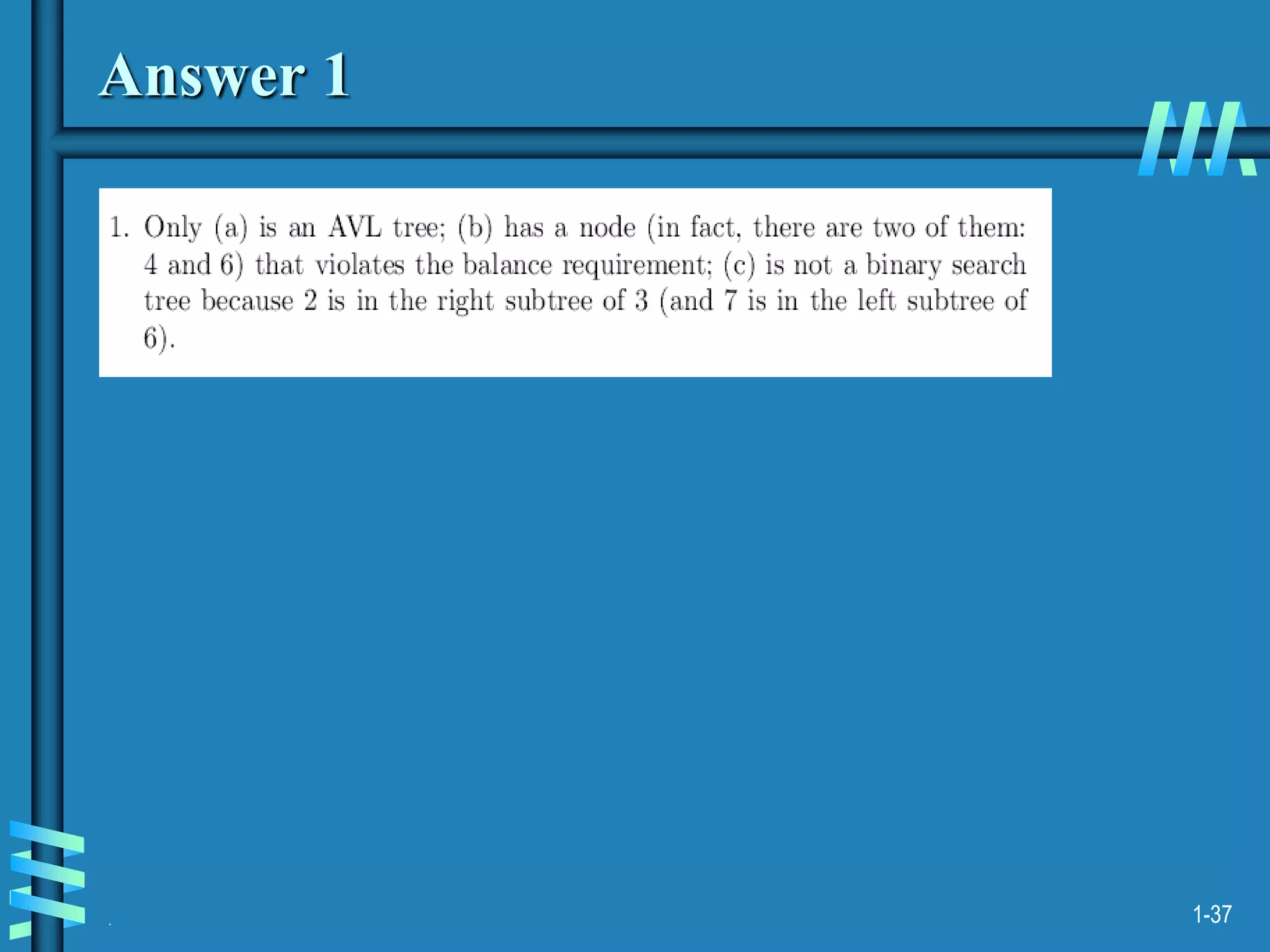
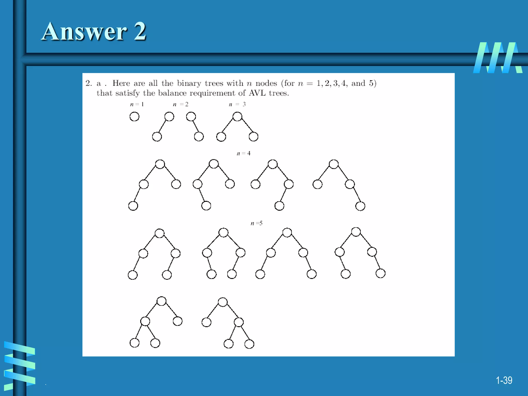
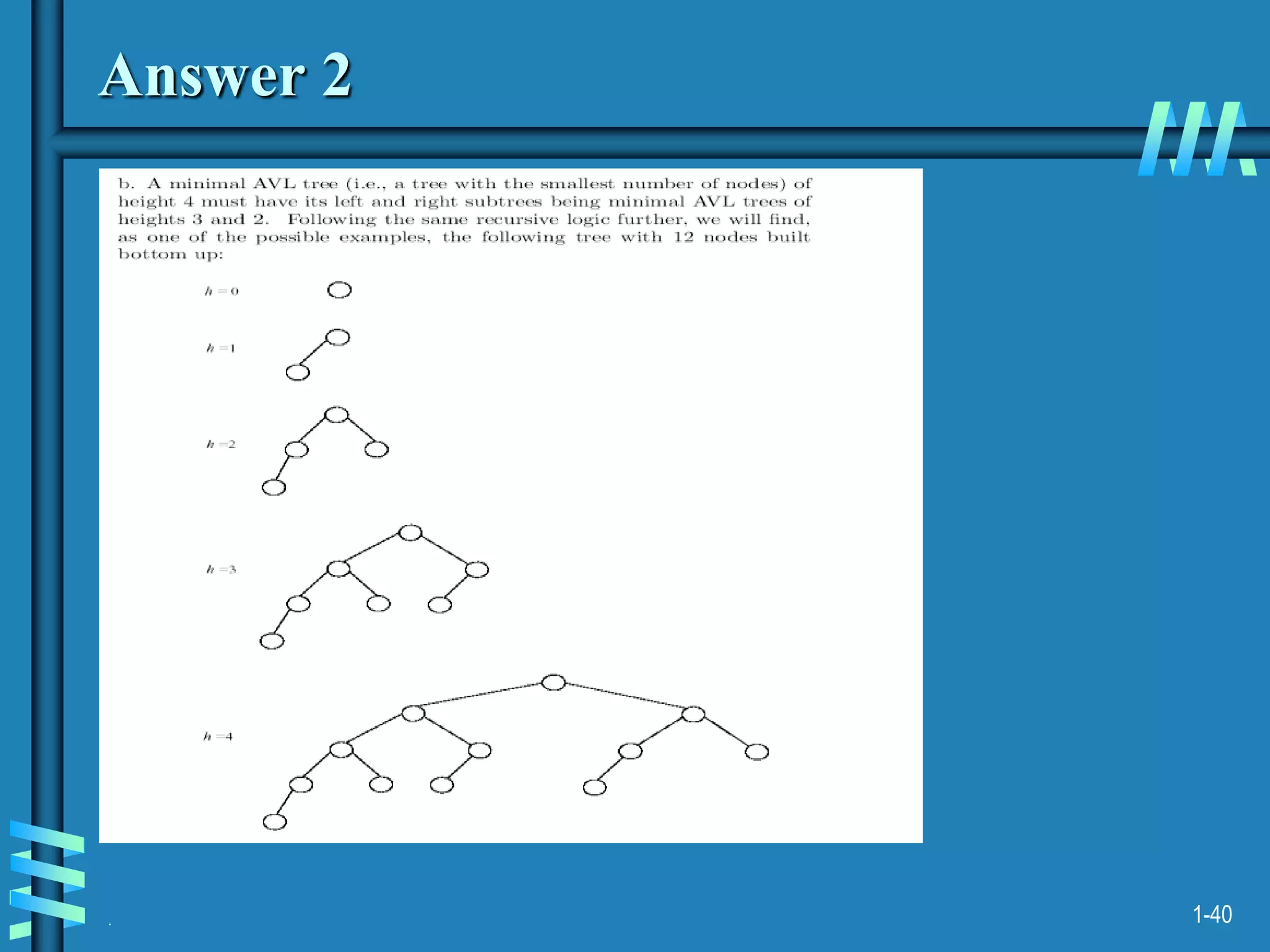
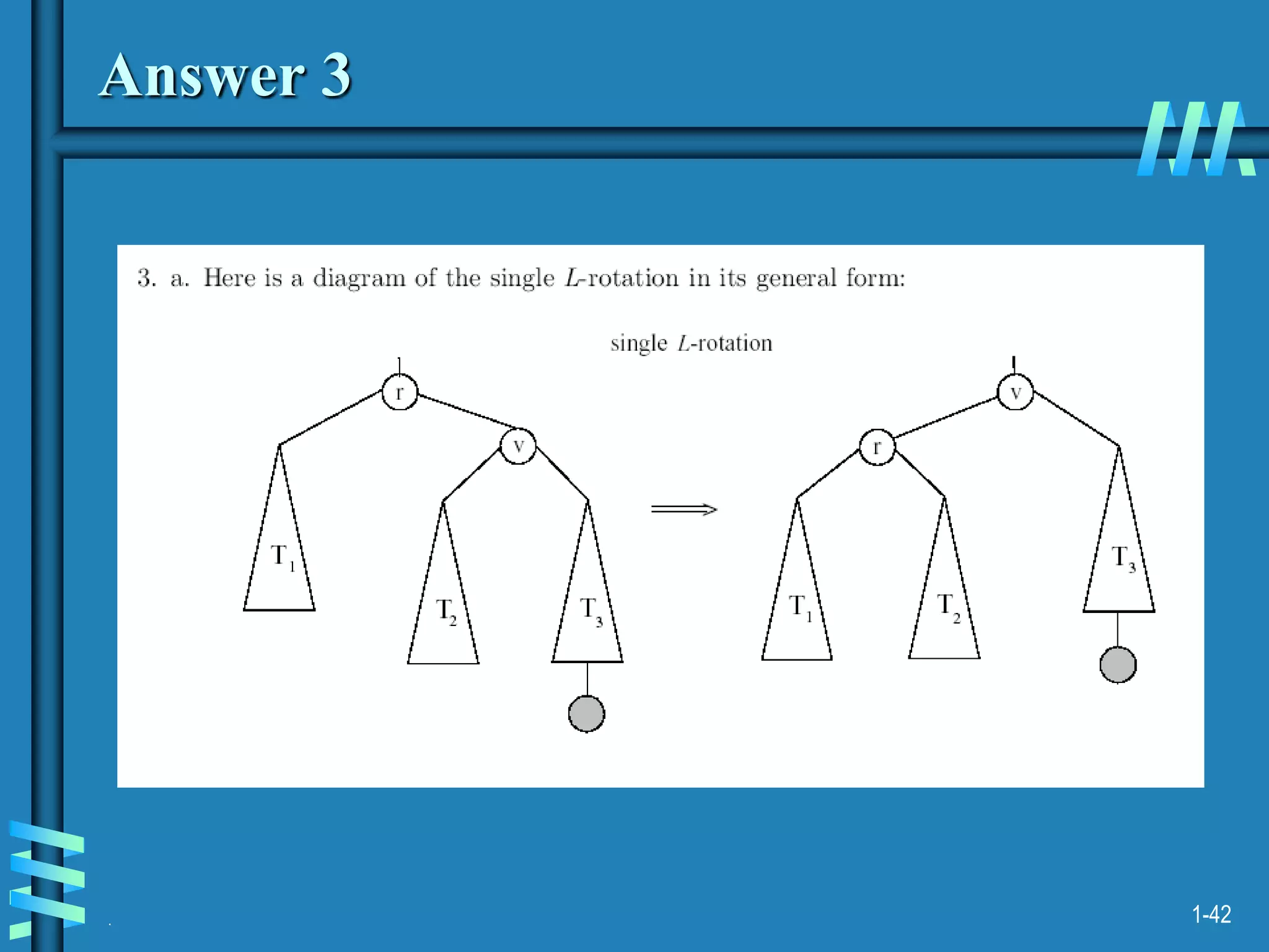
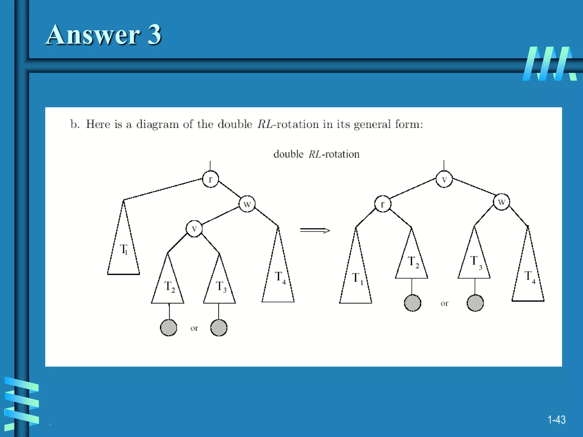
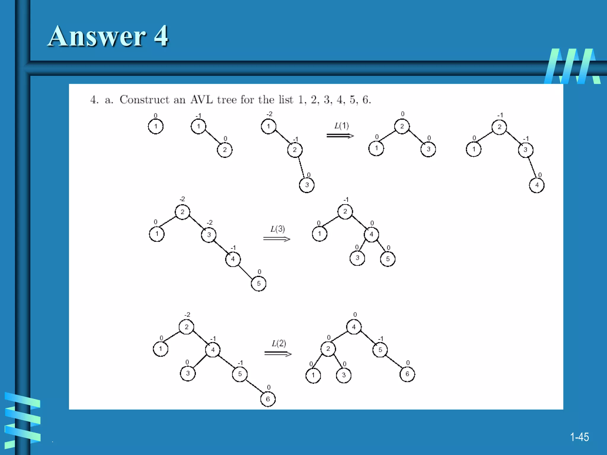
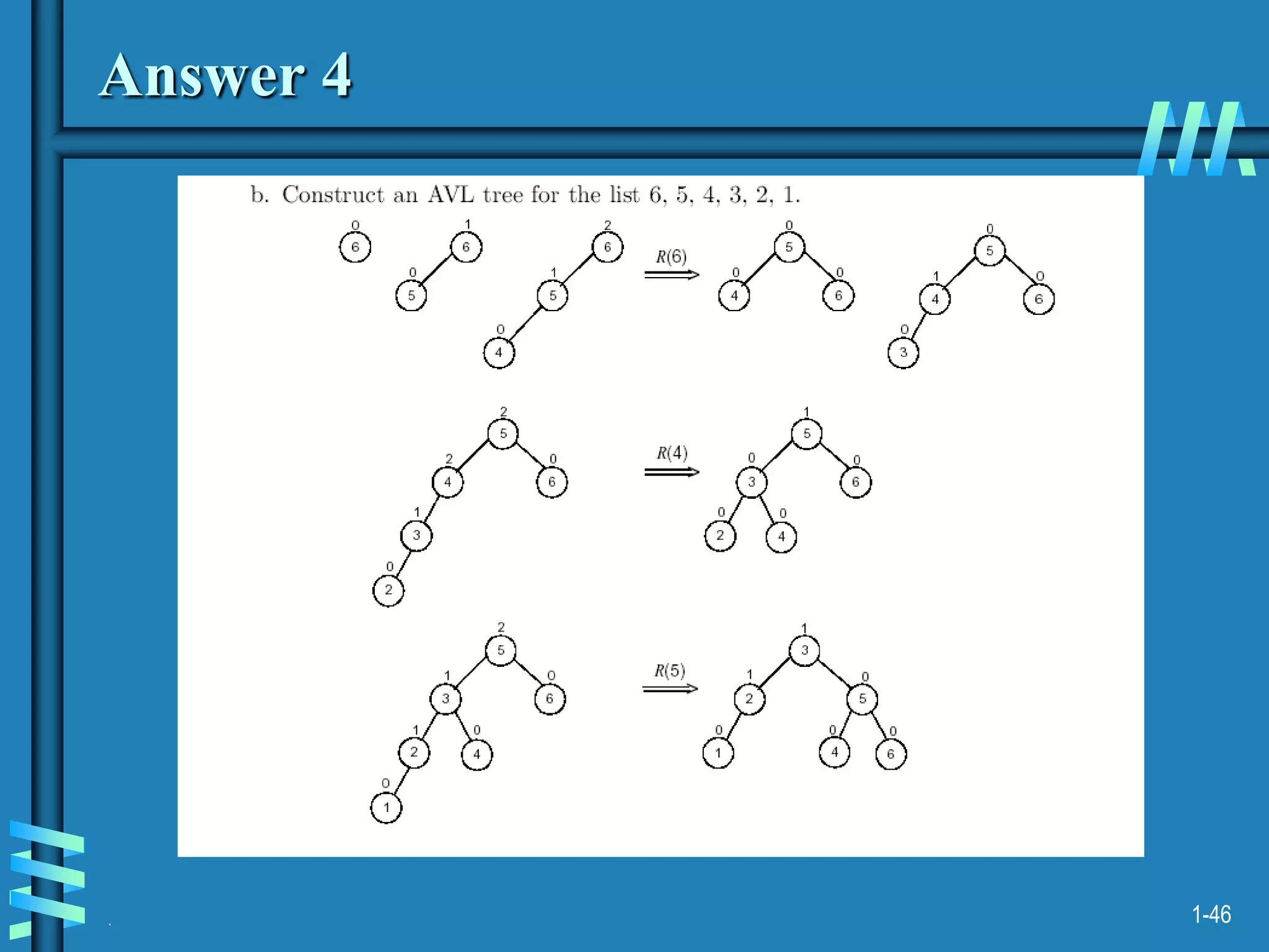
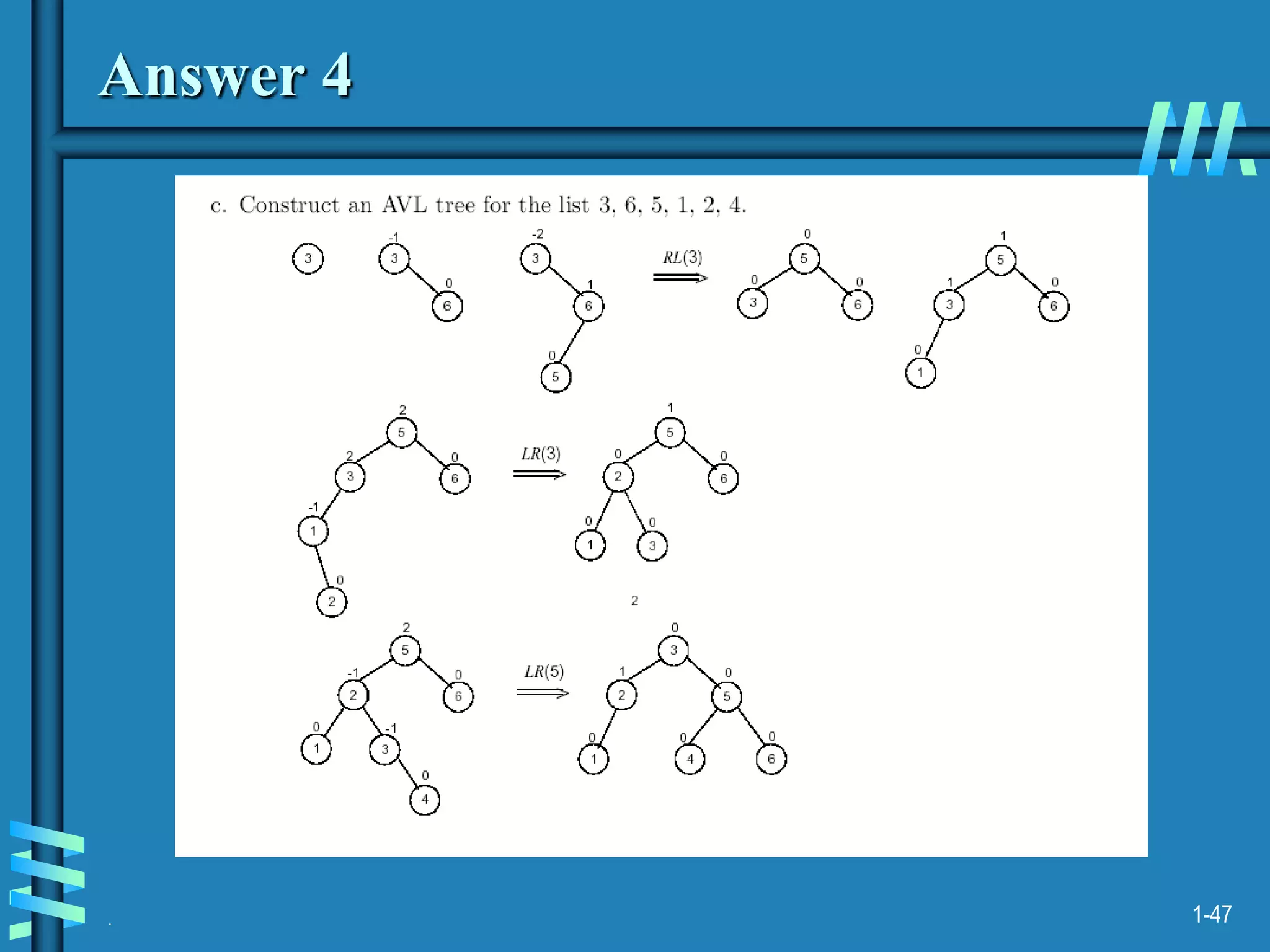
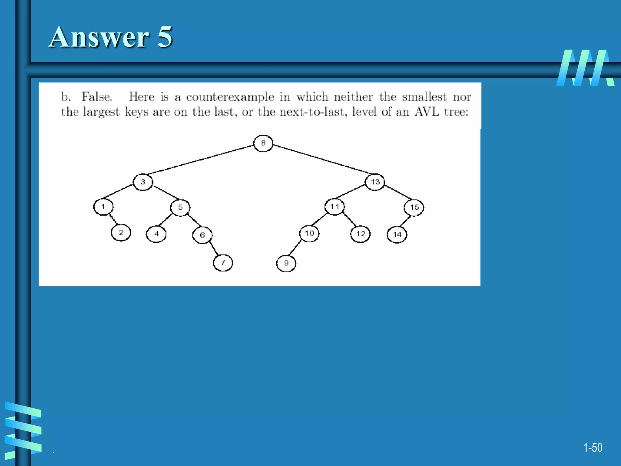
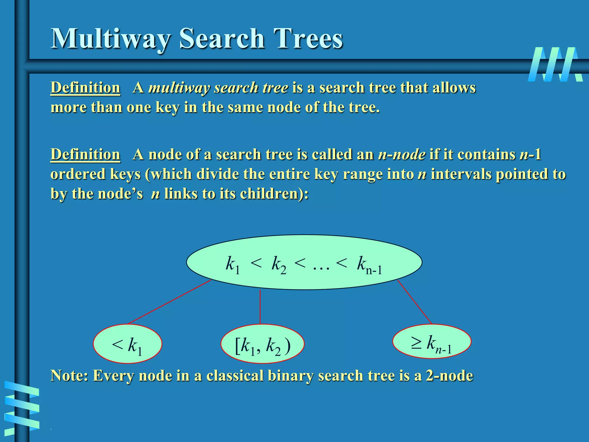
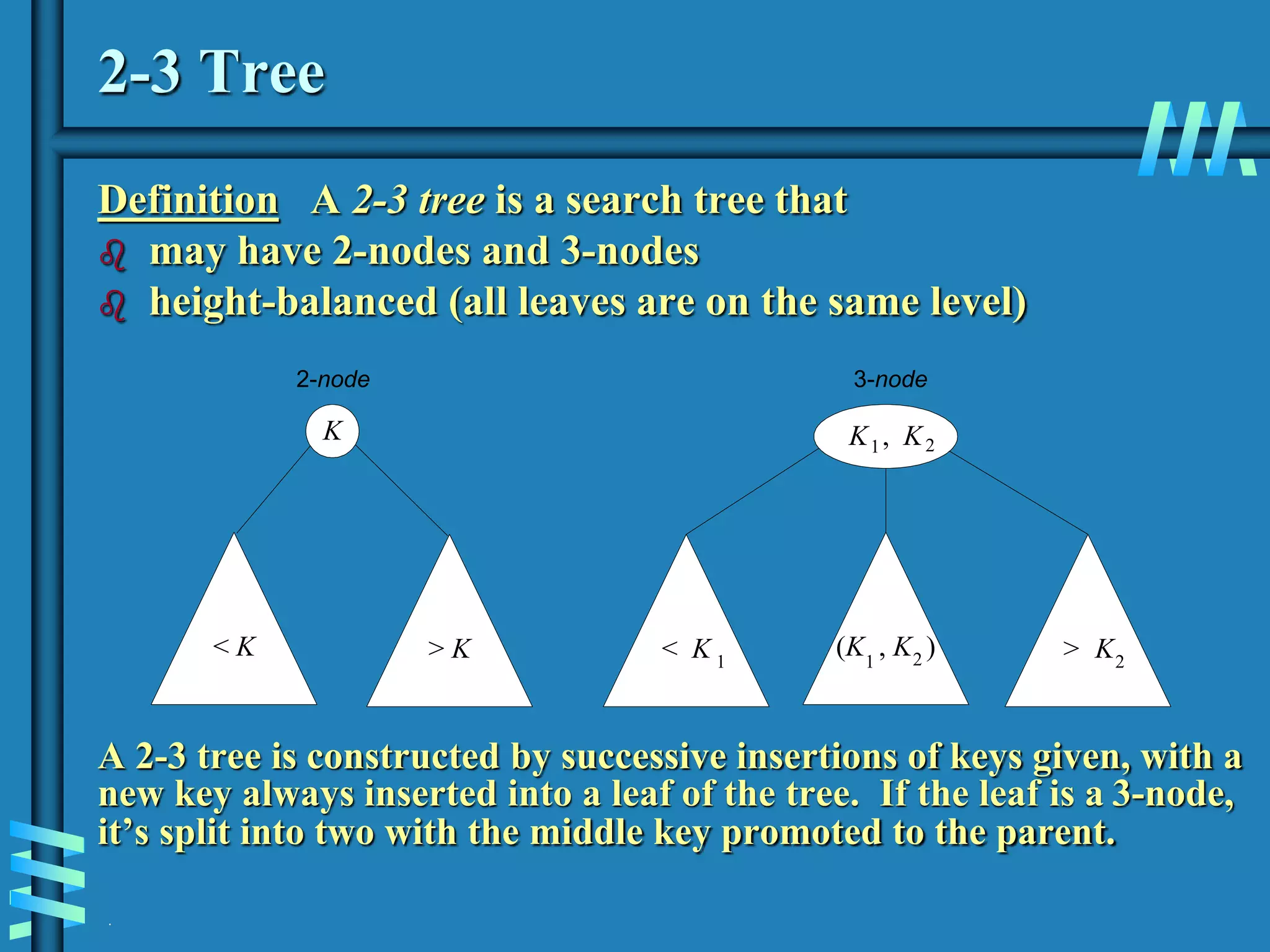
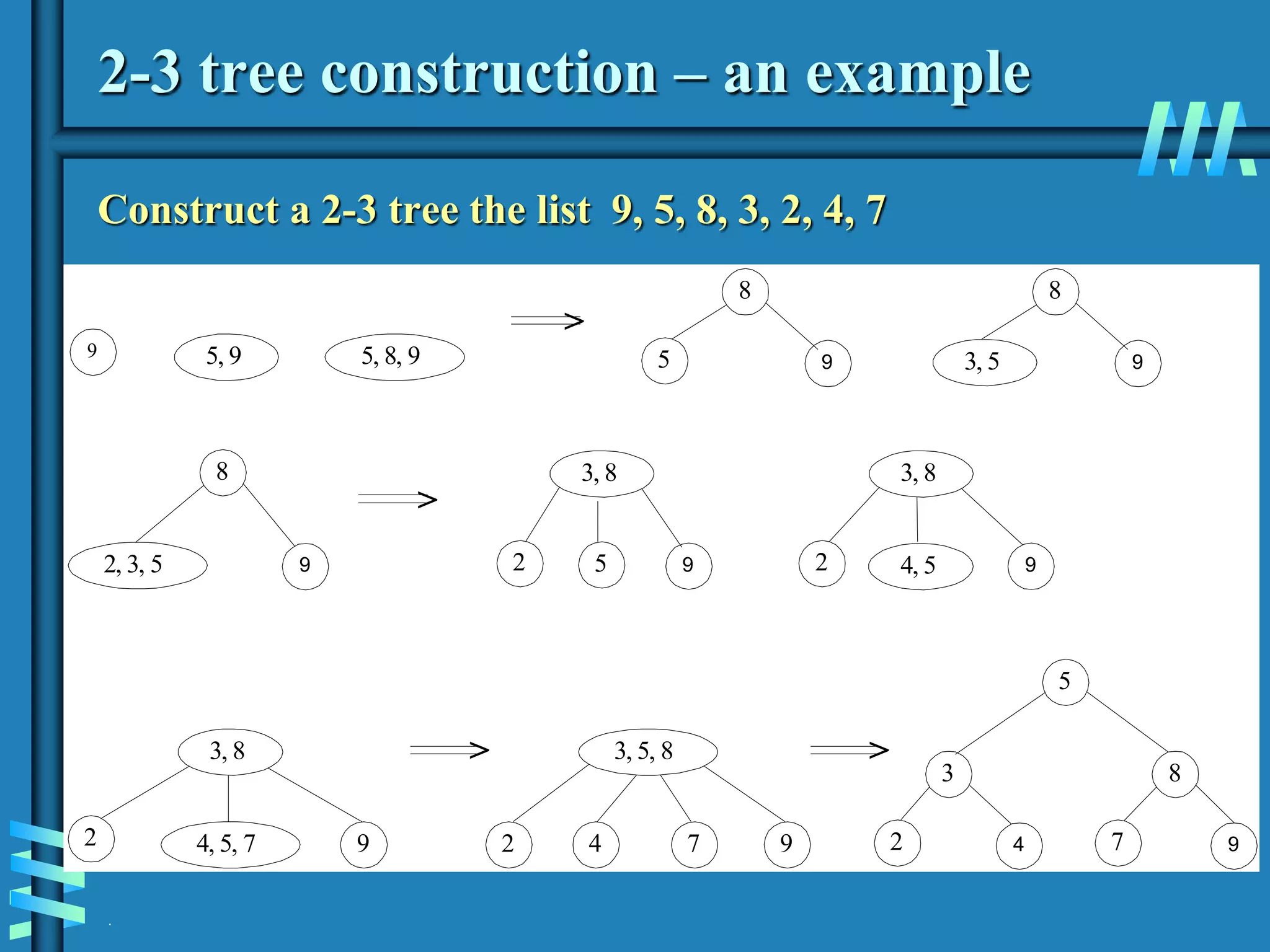
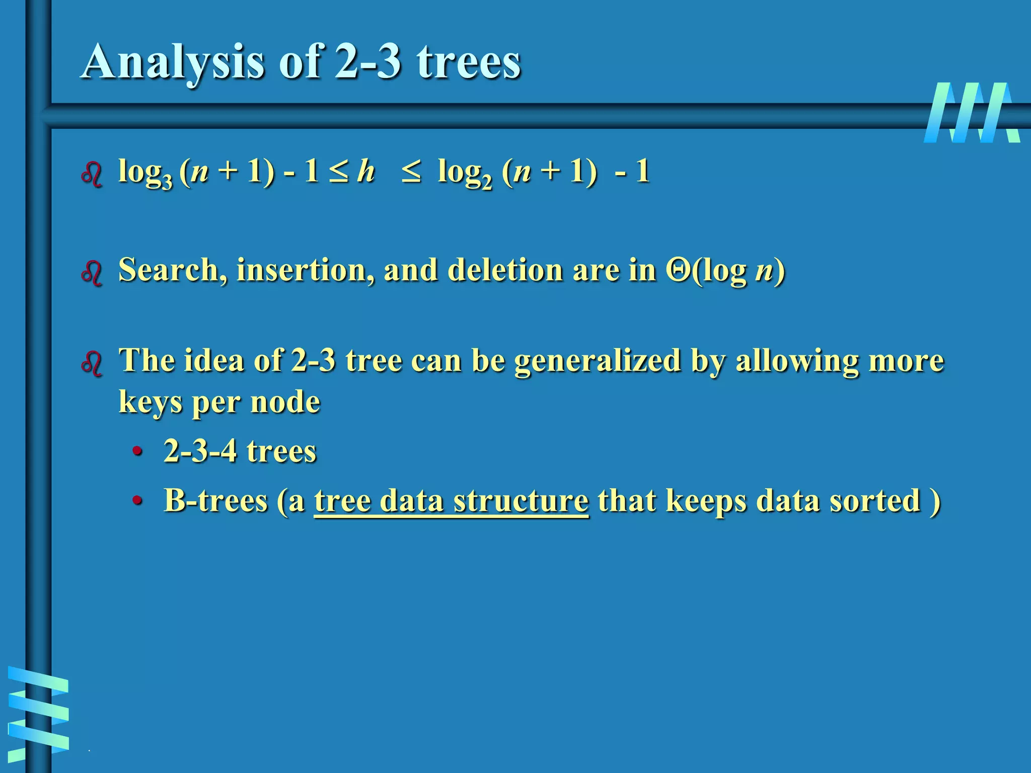
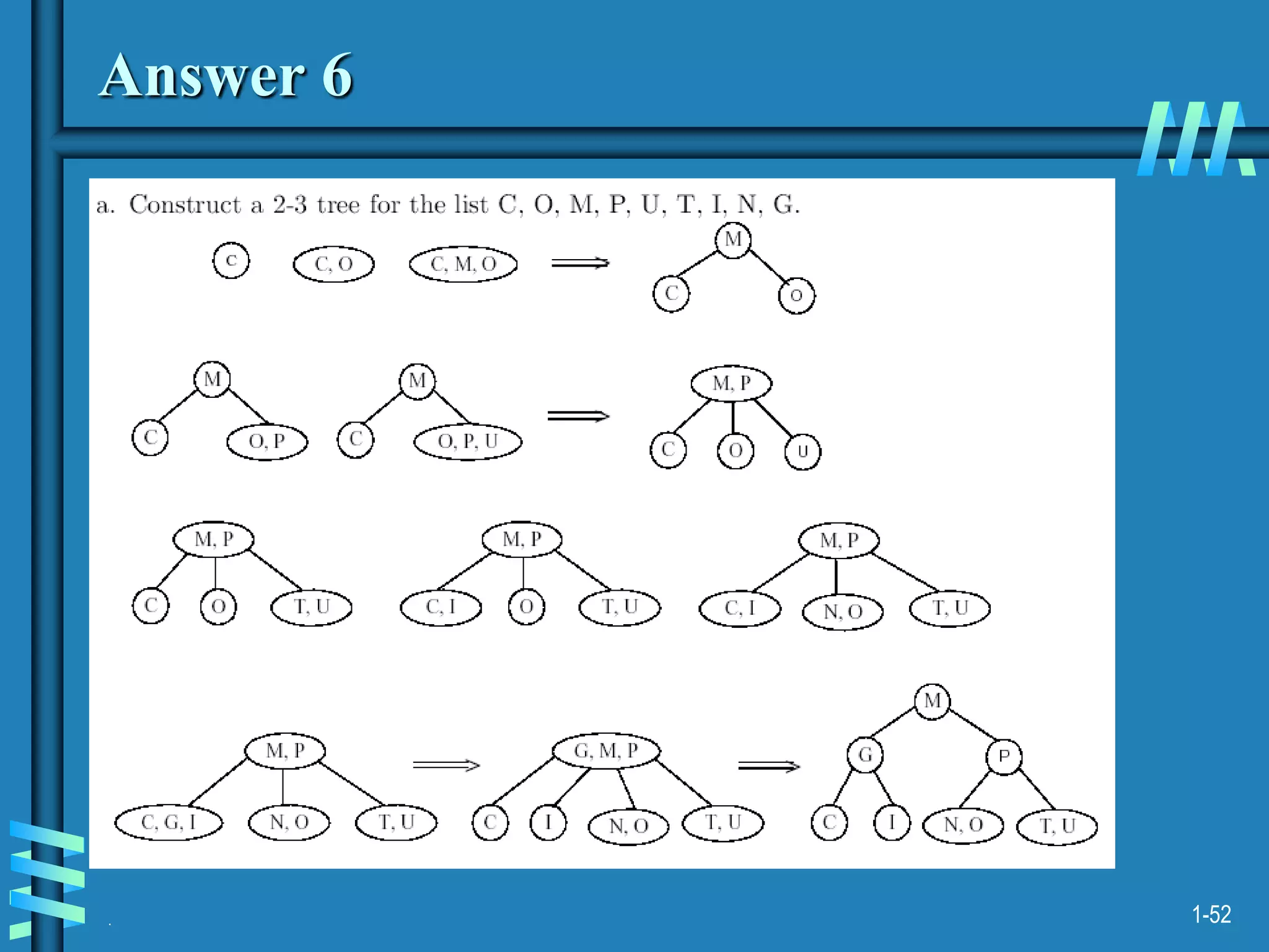
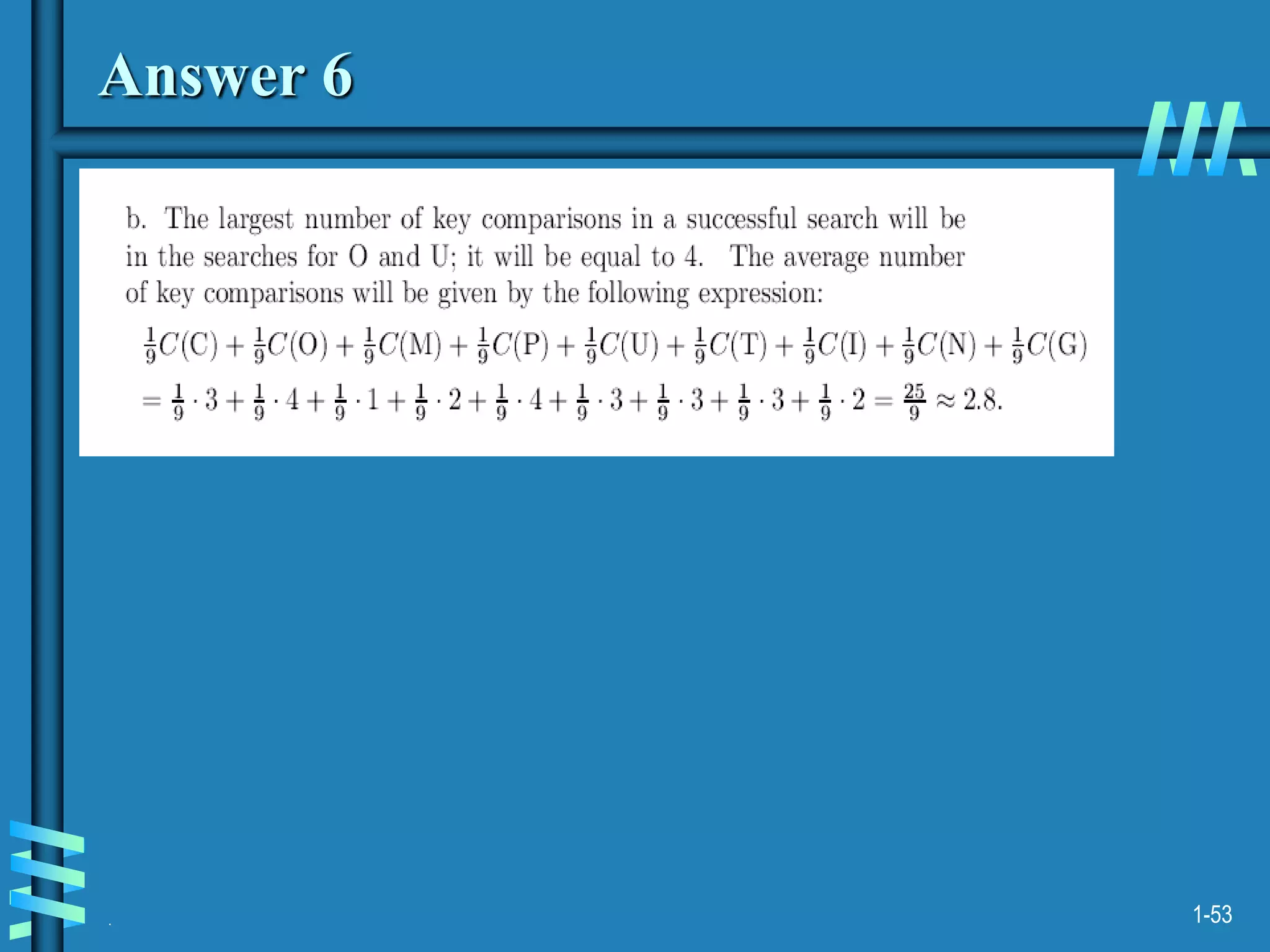
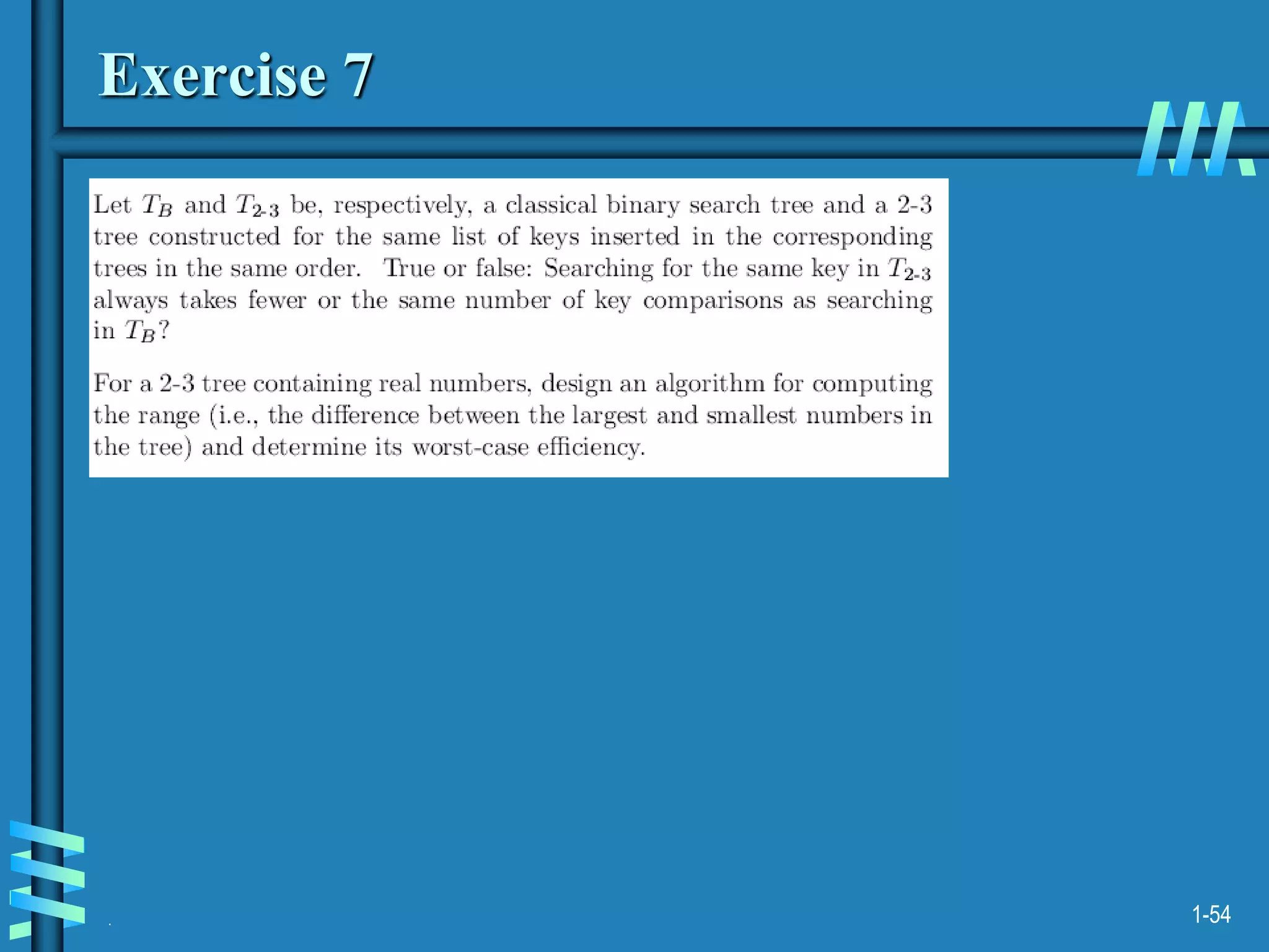
1. The document discusses algorithms for handling collisions in hashing, including open hashing which uses separate chaining with linked lists, and closed hashing which resolves collisions through techniques like linear probing. 2. It also discusses binary search trees and their operations, as well as balanced search trees like AVL and red-black trees which have logarithmic time performance. 3. Finally, it covers multiway search trees including 2-3 trees and how they allow for more than one key per node, providing improved time performance over standard binary search trees.

1. TIC424 – Complexity of
Algorithms
Prof. Magdy M. Aboul-Ela
Information Systems Department
Faculty of Management and Information Systems
French University in Egypt
Email: magdy.aboulela@ufe.edu.eg
maboulela@gmail.com
maboulela@link.net

2. The exercises are drawn from:
A. Levitin “Introduction to the Design & Analysis of
Algorithms,” 2nd ed., Copyright © 2007 Pearson
Addison-Wesley. All rights reserved.
Complexity of Algorithms
Exercises

3. .
Hash tables and hash functions
The idea of hashing is to map keys of a given file of size n into
a table of size m, called the hash table, by using a predefined
function, called the hash function,
h: K  location (cell) in the hash table
Example: student records, key = SSN. Hash function:
h(K) = K mod m where m is some integer (typically, prime)
If m = 1000, where is record with SSN= 314159265 stored?
Generally, a hash function should:
• be easy to compute
• distribute keys about evenly throughout the hash table

4. .
Collisions
If h(K1) = h(K2), there is a collision
 Good hash functions result in fewer collisions but some
collisions should be expected (birthday paradox)
• birthday paradox pertains to the probability that in a set of randomly chosen people some pair
of them will have the same birthday.
 Two principal hashing schemes handle collisions differently:
• Open hashing
– each cell is a header of linked list of all keys hashed to it
• Closed hashing
– one key per cell
– in case of collision, finds another cell by
– linear probing: use next free bucket
– double hashing: use second hash function to compute increment

5. .
Open hashing (Separate chaining)
Keys are stored in linked lists outside a hash table whose
elements serve as the lists’ headers.
Example: A, FOOL, AND, HIS, MONEY, ARE, SOON, PARTED
h(K) = sum of K ‘s letters’ positions in the alphabet MOD 13
Key A FOOL AND HIS MONEY ARE SOON PARTED
h(K) 1 9 6 10 7 11 11 12
A FOOL
AND HIS
MONEY ARE PARTED
SOON
12
11
10
9
8
7
6
5
4
3
2
1
0
Search for KID

6. .
Open hashing (cont.)
 If hash function distributes keys uniformly, average length of
linked list will be α = n/m. This ratio is called load factor.
 Average number of probes in successful, S, and unsuccessful
searches, U:
S  1+α/2, U = α
 Load α is typically kept small (ideally, about 1)
 Open hashing still works if n > m

7. .
Closed hashing (Open addressing)
Keys are stored inside a hash table.
A
A FOOL
A AND FOOL
A AND FOOL HIS
A AND MONEY FOOL HIS
A AND MONEY FOOL HIS ARE
A AND MONEY FOOL HIS ARE SOON
PARTED A AND MONEY FOOL HIS ARE SOON
Key A FOOL AND HIS MONEY ARE SOON PARTED
h(K) 1 9 6 10 7 11 11 12
0 1 2 3 4 5 6 7 8 9 10 11 12

8. .
Closed hashing (cont.)
 Does not work if n > m
 Avoids pointers
 Deletions are not straightforward
 Number of probes to find/insert/delete a key depends on
load factor α = n/m (hash table density) and collision
resolution strategy. For linear probing:
S = (½) (1+ 1/(1- α)) and U = (½) (1+ 1/(1- α)²)
 As the table gets filled (α approaches 1), number of probes
in linear probing increases dramatically:

9. .
Exercise 1
1-8

10. .
Answer 1
1-9

11. .
Exercise 2
1-10

12. .
Answer 2
1-11

13. .
Exercises 3, 4
1-12

14. .
Answer 3,4
1-13

15. .
Exercise 5
1-14

16. .
Answer 5
1-15

17. .
Exercise 6
1-16

18. .
Answer 6
1-17

19. .
Exercise 7
1-18

20. .
Answer 7
1-19

21. .
Exercise 8
1-20

22. .
Answer 8
1-21

23. .
Binary Search Tree
Arrange keys in a binary tree with the binary search
tree property:
K
<K >K
Example: 5, 3, 1, 10, 12, 7, 9

24. .
Dictionary Operations on Binary Search Trees
Searching – straightforward
Insertion – search for key, insert at leaf where search terminated
Deletion – 3 cases:
deleting key at a leaf
deleting key at node with single child
deleting key at node with two children
Efficiency depends of the tree’s height: log2 n  h  n-1,
with height average (random files) be about 3log2 n
Thus all three operations have
• worst case efficiency: (n)
• average case efficiency: (log n)
inorder traversal produces sorted list

25. .
Balanced Search Trees
Attractiveness of binary search tree is marred by the bad (linear)
worst-case efficiency. Two ideas to overcome it are:
 to rebalance binary search tree when a new insertion
makes the tree “too unbalanced”
• AVL trees
• red-black trees
 to allow more than one key per node of a search tree
• 2-3 trees
• 2-3-4 trees
• B-trees

26. .
Balanced trees: AVL trees
Definition An AVL tree is a binary search tree in which, for
every node, the difference between the heights of its left and
right subtrees, called the balance factor, is at most 1 (with
the height of an empty tree defined as -1)
5 20
12
4 7
2
(a)
10
1
8
1
0
1
0
-1
0
0
5 20
4 7
2
(b)
10
2
8
0
0
1
0
-1
0
Tree (a) is an AVL tree; tree (b) is not an AVL tree

27. .
Rotations
If a key insertion violates the balance requirement at some
node, the subtree rooted at that node is transformed via one of
the four rotations. (The rotation is always performed for a
subtree rooted at an “unbalanced” node closest to the new leaf.)
3
2
2
1
1
0
2
0
1
0
3
0
>
R
(a)
3
2
1
-1
2
0
2
0
1
0
3
0
>
LR
(c)
Single R-rotation Double LR-rotation

28. .
General case: Single R-rotation

29. .
General case: Double LR-rotation

30. .
AVL tree construction - an example
Construct an AVL tree for the list 5, 6, 8, 3, 2, 4, 7
5
-1
6
0
5
0
5
-2
6
-1
8
0
>
6
0
8
0
5
0
L(5)
6
1
5
1
3
0
8
0
6
2
5
2
3
1
2
0
8
0
>
R (5)
6
1
3
0
2
0
8
0
5
0

31. .
AVL tree construction - an example (cont.)
6
2
3
-1
2
0
5
1
4
0
8
0
>
LR (6)
5
0
3
0
2
0
4
0
6
-1
8
0
5
-1
3
0
2
0
4
0
6
-2
8
1
7
0
>
RL (6)
5
0
3
0
2
0
4
0
7
0
8
0
6
0

32. .
Analysis of AVL trees
 h  1.4404 log2 (n + 2) - 1.3277
average height: 1.01 log2n + 0.1 for large n (found empirically)
 Search and insertion are O(log n)
 Deletion is more complicated but is also O(log n)
 Disadvantages:
• frequent rotations
• complexity
 A similar idea: red-black trees (height of subtrees is allowed to
differ by up to a factor of 2)

33. .
Multiway Search Trees
Definition A multiway search tree is a search tree that allows
more than one key in the same node of the tree.
Definition A node of a search tree is called an n-node if it contains n-1
ordered keys (which divide the entire key range into n intervals pointed to
by the node’s n links to its children):
Note: Every node in a classical binary search tree is a 2-node
k1 < k2 < … < kn-1
< k1 [k1, k2 )  kn-1

34. .
2-3 Tree
Definition A 2-3 tree is a search tree that
 may have 2-nodes and 3-nodes
 height-balanced (all leaves are on the same level)
A 2-3 tree is constructed by successive insertions of keys given, with a
new key always inserted into a leaf of the tree. If the leaf is a 3-node,
it’s split into two with the middle key promoted to the parent.
K K , K
1 2
(K , K )
1 2
2-node 3-node
< K > K
< K > K 1 2

35. .
2-3 tree construction – an example
Construct a 2-3 tree the list 9, 5, 8, 3, 2, 4, 7
9
>
8
9
5
5, 9 5, 8, 9
8
9
3, 5
2, 3, 5
8
9
>
>
3, 8
9
2 5
3, 8
9
2 4, 5
3, 8
4, 5, 7
2 9
> 3, 5, 8
2 4 7 9
5
3
4
2
8
9
7

36. .
Analysis of 2-3 trees
 log3 (n + 1) - 1  h  log2 (n + 1) - 1
 Search, insertion, and deletion are in (log n)
 The idea of 2-3 tree can be generalized by allowing more
keys per node
• 2-3-4 trees
• B-trees (a tree data structure that keeps data sorted )

37. .
Exercise 1
1-36

38. .
Answer 1
1-37

39. .
Exercise 2
1-38

40. .
Answer 2
1-39

41. .
Answer 2
1-40

42. .
Exercise 3
1-41

43. .
Answer 3
1-42

44. .
Answer 3
1-43

45. .
Exercise 4
1-44

46. .
Answer 4
1-45

47. .
Answer 4
1-46

48. .
Answer 4
1-47

49. .
Exercise 5
1-48

50. .
Answer 5
1-49

51. .
Answer 5
1-50

52. .
Exercise 6
1-51

53. .
Answer 6
1-52

54. .
Answer 6
1-53

55. .
Exercise 7
1-54

56. .
Answer 7
1-55