This document presents a major project on heat transfer study using COMSOL Multiphysics software. It was submitted by Suraj Kumar and Pankaj Kumar to the Department of Chemical Engineering at Sant Longowal Institute of Engineering & Technology to fulfill the requirements for a Bachelor of Engineering degree in Chemical Engineering. The project involves simulating a heat exchanger model in COMSOL to calculate the heat transfer coefficient and pressure drops. It includes sections on objectives, literature review on heat transfer mechanisms and heat exchangers, an overview of the COMSOL software, the heat exchanger modeling procedure, and conclusions.

1. MAJOR PROJECT
ON
HEAT TRANSFER STUDY IN
COMSOL MULTYPHYSICS
BY
SURAJ KUMAR GCT-1731671
PANKAJ KUMAR GCT1731674
Submitted to the department of chemical Engineering
In partial fulfilment of the requirements
for the degree of
Bachelor of Engineering
In
Chemical engineering
Sant Longowal institute of engineering & technology
Deemed university Longowal, Distt. Sangrur
June 2020

2. ii
CERTIFICATION
This is to certify that work presented in the project titled ‘HEAT TRANSFER STUDY IN
COMSOL MULTYPHYSICS’ submitted to the department of Chemical Technology of SLIET
is an authentic record of our own work carried out during the period of 8th semester under
supervision of project guide Dr. AMIT RAI, Department of Chemical Technology, SLIET.
SURAJ KUMAR _GCT-1731671 …………….
PANKAJ KUMAR _GCT-1731674 .…………....
………………………… …..……………………….
(Sign. Of Project Guide) (Sign. Of Project In-charge)
…………………………….
(Sign. Of H.O.D.)

3. iii
DECLARATION
I the undersigned solemnly declare that the project report” HEAT TRANSFER STUDY IN
COMSOL MULTYPHYSICS’ is based on my own work carried out during our study under
the supervision of Dr. AMIT RAI.
I assert the statements made and conclusions drawn are an outcome of my research work. I
further certify that
I. The work contained in the report is original and has been done by me under the general
supervision of my supervisor.
II. The work has not been submitted to any other Institution for any other
degree/diploma/certificate in this university or any other University of India or abroad.
III. We have followed the guidelines provided by the university in writing the report.
IV. Whenever we have used materials (data, theoretical analysis, and text) from other
sources, we have given due credit to them in the text of the report and giving their details
in the references.
NAME OF STUDENT
SURAJ KUMAR: -GCT-1731671 ……………………………….
PANKAJ KUMAR: -GCT-1731674 ……………………………….
DATE: -28-06-2020

4. iv
ACKNOWLEDGEMENTS
We would like to express profound gratitude and appreciation to our project guide Dr. AMIT
RAI and our project in-charge Dr. PUSHPA JHA for his invaluable support, encouragement,
supervision and useful suggestions throughout the project work. His moral support and continuous
guidance enabled us to overcome our dough and complete our work successfully
We are grateful for the cooperation and constant encouragement from our honourable Head
of Department of chemical technology Dr. AVINASH THAKUR His regular suggestions made
our work easy and proficient.
Last but not least, I am thankful and indebted to all the faculty members of chemical
department and friends who helped us directly or indirectly in completion of this project.

5. v
ABSTRACT
This thesis used the study of Heat Transfer and COMSOL Multiphysics software as a reference
which was made for the purpose of future education in engineering field. The main reason to
apply COMSOL Multiphysics software into heat transfer processes. It consists of a general view
of three mechanisms of heat transfer: conduction, convection and radiation. which were presented
in this thesis. In this project to study the software and It presented two methods of the performance
to solve the three basic heat transfer problem. A simulation of Heat Exchanger heat transfer
process was performed by COMSOL Multiphysics in order to calculate the heat transfer
coefficient, and pressure drop inlet or outlet. To validate the data from experimental and
theoretical.

6. vi
Article I. TABLE OF CONTENTS
CERTIFICATION …………………………………………………………….... ii
DECLARATION………………………………………………………. iii
ACKNOWLEDGEMENTS......................................................................................... iv
ABSTRAC……………………………………………………………… v
TABLE OF CONTENTS .............................................................................................. 4
LIST OF FIGURES....................................................................................................... 6
LIST OF TABLES ..................................................................................................................7
LIST OF SYMBOLS .................................................................................................... 8
1 INTRODUCTION..................................................................................................... 1
1.1 Background............................................................................................................. 1
1.2 Purpose.................................................................................................................. 10
1.3 Thesis Outline ......................................................................................................... 2
2 OBJECTIVES............................................................................................................ 4
3 LITERATURE SURVEY...................................................................................................5
3.1 Overview of Heat Transfer ..................................................................................... 5
3.1.1 Conduction Heat Transfer.....................................................................................6
3.1.1.1 Conduction rate equation ........................................................................... 6
3.1.1.2 Partial Differential Equation of Heat Conduction...................................... 7
3.1.2 Convection Heat Transfer .................................................................................... 9
3.1.2.1 Newton’s law of cooling........................................................................... 10
3.1.2.2 Overview of fluid mechanics................................................................... 10
3.1.2.3 Convection Transfer Equation ................................................................. 12
3.1.2.4 The convection coefficients ..................................................................... 15
3.1.3 Radiation Heat Transfer ..................................................................................... 15
3.1.3.1 Properties of radiation.............................................................................. 16
3.1.3.2 Stefan-Boltzmann law of thermal radiation ............................................. 16
3.1.3.3 Radiation Energy Exchange..................................................................... 17

7. vii
3.2 Heat exchanger ..................................................................................................... 18
3.2.1 Working theory of Heat exchanger................................................................. 18
3.2.2 Heat exchangers used for......................................................................... 19
3.2.3 Types of Heat Exchanger…………………….………...……… 19
4 COMSOL Multiphysics Software ........................................................................... 21
4.1 COMSOL Multiphysics software………………………………………………. 21
4.1.1 History ........................................................................................................... 21
4.1.2 application areas ............................................................................................. 21
4.1.3 Characteristics ................................................................................................ 21
4.2 Problem solving process........................................................................................ 22
4.2.1 solving systems of coupled nonlinear PDEs that can include ........................ 22
4.2.2 Modeling process............................................................................................ 22
5 Heat Exchanger model procedure.....................................................................................25
5.1 how to model heat Exchanger problems............................................................... 25
5.2 Simulating shell & tube HE .................................................................................. 25
5.3 Step of Simulating Model ..................................................................................... 26
5.4 Model Definition................................................................................................... 31
5.5 Boundary Condition.............................................................................................. 32
5.6 Result & Discussion.............................................................................................. 33
6 CONCLUSION ....................................................................................................... 37
7 REFERENCES........................................................................................................ 38

8. viii
Article II. LIST OF FIGURES
Figure 1. Conduction heat transfer ................................................................................. 6
Figure 2. Conduction analysis in Cartesian coordinates................................................. 7
Figure 3. Conduction analysis in Cylindrical coordinates.............................................. 8
Figure 4. Conduction analysis in Spherical coordinates................................................. 9
Figure 5. Convection heat transfer.................................................................................. 10
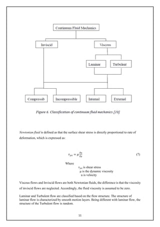
Figure 6. Classification of continuum fluid mechanics .................................................. 11
Figure 7. Velocity boundary layer development on a flat plate ...................................... 13
Figure 8. Thermal boundary layer development on a flat plate...................................... 13
Figure 9. Effects of incident radiation]........................................................................... 16
Figure 10. Radiator heated from range boiler................................................................. 31
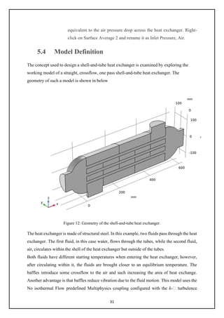
Figure 11. Geometry of the shell-and-tube heat exchanger ............................................ 26
Figure 12. Geometry of the shell-and-tube heat exchanger .................................................. 32
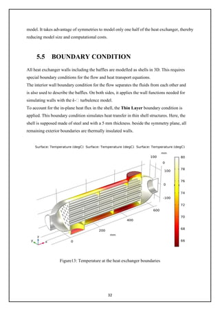
Figure 13. Temperature at the heat exchanger boundary................................................ 33
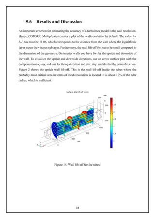
Figure 14. Wall lift-off for the tubes.................................................................................. 34
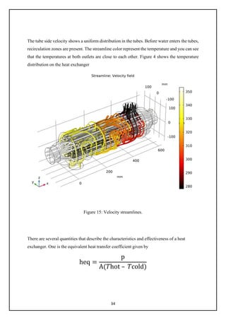
Figure 15. Velocity streamlines...................................................................................... 34

9. ix
Figure 16. over all heat transfer coefficient.................................................................... 35
Figure 17. pressure Drop tube side ................................................................................. 35
Figure 18. pressure Drop tube side ................................................................................. 36

10. x
Article III. LIST OF SYMBOLS
A Area
α Absorptivity
c Specific Heat at constant pressure
E Energy
E Emissive power
Eb Blackbody emissive power
X, Y Force
G Irradiation
h Heat transfer coefficient
J Radiosity
k Thermal conductivity
L Length
p Pressure
q Heat transfer rate
q'' Heat flux
Heat generated per unit volume
Q Heat
u, v, w Velocity
ε emissivity
μ Dynamic viscosity
ρ Density
ρ Reflectivity
σ Stefan-Boltzmann
t Time
τ Transmissivity
τyx Shear stress
T Temperature

11. 1
1 INTRODUCTION
1.1 Background
Since 1970s, the energy crisis has been listed in the five most essential worldwide problems.
And the other four problems are respectively people, food, environment, and resource. In
this situation, energy saving becomes more important than ever. People are encouraged to
contribute on sustainable development in daily life.
The finite element method is a numerical technique that gives approximate solution to
differential equations that model problems arising in physics and engineering. As with the
more commonly used finite difference scheme, the finite element method reduced problems
defined in geometrical space, to finding a solution in a finite number of points by
subdividing the domain into smaller region. In finite difference methods in the past, the
mesh consisted of rows and columns of orthogonal lines (in computational space – a
requirement now relaxed through the use of coordinate transformation and unstructured
mesh generators); in finite elements, each subregions or “element” is unique and needed not
be orthogonal to the others.
Heat transfer has been widely used nowadays. Therefore, it is important for an engineer to
have related knowledge on heat transfer. At the same time, following with the boom of the
computer technology, certain types of Computer Software have been introduced for the
purpose of analyzing heat transfer efficiently. COMSOL Multiphysics software is one of
them, which has been taken as a helpful tool for making analysis on the processes of heat
transfer. In this thesis, the author introduces COMSOL Multiphysics software and analyzes
heat transfer processes.

12. 2
1.2 Purpose
There are mainly two purposes of this thesis. The first one is to give implications to future
engineering students. The author introduces about heat transfer and ways of using
COMSOL Multiphysics software to solve some problems. By doing so, this study is
supposed to act as a foundation of further researches with the same subject. The second
purpose is to put the knowledge into practice. The author applies the COMSOL
Multiphysics software to simulate the Heat Exchanger heat transfer process so that the
Heat Exchanger’ heat transfer coefficient can be calculated. Based on the analysis of the
process, the author makes descriptions on the ways of improving Heat Exchanger heat
transfer coefficient.
1.3 Thesis Outline
Theoretical chapter. In this chapter, we firstly introduce about definition of heat transfer.
Then, it follows with descriptions about three basic transfer models: conduction,
convection, and radiation. Meanwhile, there is a further discussion on the three models.
Afterwards, the author gives an introduction about heat exchanger, which is taken as an
example of saving energy from heat transfer process. The principle of work and the type
of heat exchanger are mainly presented. Comes up with the last part of the theoretical
review, it refers to the COMSOL Multiphysics’s software. This part mentions about the
software’s historical development, functions and some other related characteristics.
The other two chapters of the thesis are Method and Results, which are two most essential
parts of the thesis. In the first part of the Method chapter, the we choose three basic heat
transfer problems, which relates to three heat transfer models, and then solves them by

13. 3
theoretical method and COMSOL Multiphysics software. In the second part, the author
establishes a model simulation of a Heat Exchanger. According to the definition of
conduction, convection, and radiation, it is proved that the process of heat transfer contains
all the three heat transfer models. Based on this knowledge, the author establishes a model
with the help of COMSOL Multiphysics software. The heat transfer coefficient of Heat
Exchanger is supposed to be calculated according to the simulated temperature distribution.
Finally, the results of the basic heat transfer problems and heat transfer coefficient of Heat
Exchanger are stated in the Results chapter.
solves them by theoretical method and COMSOL Multiphysics software. In the second
part, based on this knowledge, we establish a model with the help of COMSOL Multiphysics
software. The heat transfer coefficient of the Heat Exchanger is supposed to be calculated
according to the simulated room’s temperature distribution. Finally, the results of the three
basic heat transfer problems and heat transfer rate are stated in the Results chapter.
Conclusion is the last part of the thesis. In this part, the author compares the results of
three problems obtained by theoretical method and COMSOL Multiphysics software. A
conclusion about the main factors of affecting the heat transfer process of a Heat
Exchanger is stated. Furthermore, there is a conclusion about the simulation results, which
is obtained from model simulation.

14. 4
2 OBJECTIVES
There are five main objectives in total, which have been stated as followings:
1. To offer a clearly introduction about three mechanisms of heat transfer:
 Conduction
 Convection
 Radiation
2. To provide a general introduction to COMSOL Multiphysics software
3. To simulate the heat transfer processes between fluid to air by using COMSOL
Multiphysics software.
4. To compute heat transfer coefficient in Heat Exchanger.

15. 5
3 LITERATURE SURVEY
3.1 Overview of Heat Transfer
Temperature is a common phenomenon in nature. And it was used to describe the hot and
cold. From the perspective of micro-physical, the temperature stands for the intensity of
molecular motion. According to Holman, energy transfer happens while temperature
difference exists between material bodies. Heat transfer is such a science to be used for
estimating the energy transfer.
When the temperature difference exists between material bodies, heat is always transferred
from the hotter object to the colder one. In other worlds, heat never goes from a colder object
to a warmer object. The transfer of the heat can be discovered from everywhere in people’s
daily life. For instance, the temperature of hot water starts to drop if putting an ice into the
cup. This is because that the temperature of the water is higher than the ice so that heat is
transferred from the water to the ice.
Heat transfer has been applied widely in various fields, there are mainly three research fields
can be generated. These three aspects are:
1) How to increase the hate transfer rate.
2) How to decrease the hate transfer rate.
3) How to keep the temperature in certain range.
Heat transfer has three basic transfer models: conduction, convection and radiation. Regards
to the study of heat transfer; it is divided into these three parts in this study well. accordingly,
these three parts are introduced here only by one in detail.

16. 6
3.1.1 Conduction Heat Transfer
Conduction is a process of heat transfer generated by molecular vibration within an
object. The object has no motion of the material during the heat transfer process. The
example below well explained about conduction heat transfer. [5]
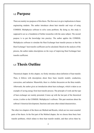
Figure 1. Conduction heat transfer
As Figure 1, there is a metal stick. Using a candle to heat the left side of the stick for a
while, then the right side of the stick will be found to be hot as well. It is because the
energy has been transferred from the left side of the stick to the right side. And this kind
of heat transfer is conduction.
3.1.1.1 Conduction rate equation
After knowing a subject’s conduction is the heat transfer from one end to the other end, it
is important for calculating about the heat transfer rate. Based on the experiment
experiences, for the one dimension conduction heat transfer in a plane wall, the amount
of heat energy being transferred per unit time is proportional to the normal temperature
gradient
𝑑𝑑𝑑𝑑
𝑑𝑑𝑑𝑑
and the cross-sectional area A [7, p4], this can be expressed as:
𝑞𝑞 = −𝑘𝑘𝑘𝑘
𝑑𝑑𝑑𝑑
𝑑𝑑𝑑𝑑
(1)
Where: -
q is the heat-transfer rate, W
A is cross-sectional area, m2
k is the thermal conductivity of the material, W/ (m.K)

17. 7
dT
dx
is the temperature gradient
The Equation (1) is the formula of calculation of conduction heat transfer rate; it is also known
as Fourier’s law of heat conduction. The minus sign means heat transferred in the direction of
decreasing temperature. If the heat transfer rate q divided by the cross-sectional area A, the
equation (1) can be derived as:
𝑞𝑞" = −𝑘𝑘
𝑑𝑑𝑑𝑑
𝑑𝑑𝑑𝑑
(2)
Where， q‫״‬ called conduction heat flux. The heat flux was derived from the Fourier’s law of
heat conduction; it can be described as the heat transfer rate through unit cross-sectional area.
The amount of the thermal conductivity k indicates the substance’s ability of transferring heat.
If it is a big amount, it means the substance has high level of ability on heat transfer. The
number of the thermal conductivity depends on the material; of course, it is also affected by
the temperature outside. In the last part of the thesis, the heat transfer situation is observed by
setting different thermal conductivities when simulating the heat transfer processes between
fluid to Air.
3.1.1.2 Partial Differential Equation of Heat Conduction
Refers to the research on conduction, one of the most important purposes is to know how the
temperature is distributing in the medium. Once the distribution situation of the temperature is
known, the heat transfer rate can be calculated.
To derive a mathematical formulation of temperature distribution, both the law of the
conservation of energy and the Fourier’s law should be used. On the basis of conservation of
energy, the balance of heat energy for a medium expressed as
[Energy conducted from outside of the medium] + [Heat generated within medium] =
[Energy conducted to outside of the medium] + [Change in internal energy within
medium]
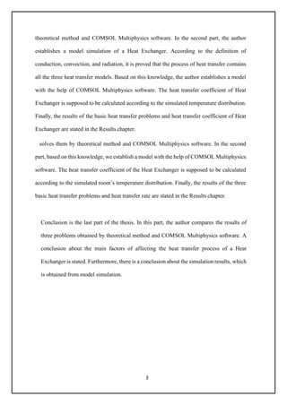
Figure 2. Conduction analysis in Cartesian coordinates

18. 8
Figure 2 shows the heat-conduction energy balance in a Cartesian coordinate.
Based on the heat-conduction energy balance, the following equation was derived [7 p56]:
𝜕𝜕
𝜕𝜕𝜕𝜕
�𝑘𝑘
𝜕𝜕𝜕𝜕
𝜕𝜕𝜕𝜕
� +
𝜕𝜕
𝜕𝜕𝜕𝜕
�𝑘𝑘
𝜕𝜕𝜕𝜕
𝜕𝜕𝜕𝜕
� +
𝜕𝜕
𝜕𝜕𝜕𝜕
�𝑘𝑘
𝜕𝜕𝜕𝜕
𝜕𝜕𝜕𝜕
� + 𝑞𝑞° = 𝜌𝜌𝜌𝜌
𝜕𝜕𝜕𝜕
𝜕𝜕𝒕𝒕
(3)
Where: -
𝜌𝜌 is density, kg/m3
C is the specific heat of material, 𝐽𝐽 𝑘𝑘𝑘𝑘. 𝐾𝐾
⁄
𝑞𝑞° is the Heat generated per unit volume, W/m3
Equation (3) is called differential equation of heat conduction; it is also called heat diffusion
equation. This equation describes the process of the general conduction heat transfer in
mathematical method. When applying the equation to solve problems, the equation (3) will be
simplified in accordance with the requirement of question and boundary conditions. Three
common boundary conditions show as following:
a) Constant surface temperature:
T (0, t) =Ts
b) Constant surface heat flux:
−k
∂T
∂x
= qs"
c) Convection surface condition:
−k
∂T
∂x
x = 0 = h[x = 0 = h [(T∞ − T(0, t)]
The heat equation (3) was expressed in a Cartesian coordinate. For cylindrical coordinates and
spherical coordinates, the heat conduction energy balance is shown in Figure 3 and Figure 4.
The heat diffusion equation is expressed as equation (4) and (5).
Figure 3. Conduction analysis in Cylindrical coordinates

19. 9
Cylindrical Coordinates]:
1
𝑟𝑟
𝜕𝜕
𝜕𝜕𝜕𝜕
�𝑘𝑘𝑘𝑘
𝜕𝜕𝜕𝜕
𝜕𝜕𝜕𝜕
� +
1
𝑟𝑟2
𝜕𝜕
𝜕𝜕∅
�𝑘𝑘
𝜕𝜕𝜕𝜕
𝜕𝜕∅
� +
𝜕𝜕
𝜕𝜕𝜕𝜕
�𝐾𝐾
𝜕𝜕𝜕𝜕
𝜕𝜕𝜕𝜕
� + 𝑞𝑞° = 𝜌𝜌𝜌𝜌
𝜕𝜕𝜕𝜕
𝜕𝜕𝜕𝜕
(4)
Where: -
𝜌𝜌 is density, kg/m3
C is the specific heat of material, J/kg. K
𝑞𝑞 ∙ is the energy generated per unit volume, W/m3
Figure 4. Conduction analysis in Spherical coordinates
Spherical Coordinates: -
1
𝑟𝑟
𝜕𝜕
𝜕𝜕𝜕𝜕
�𝑘𝑘𝑘𝑘
𝜕𝜕𝜕𝜕
𝜕𝜕𝜕𝜕
� +
1
𝑟𝑟2
𝜕𝜕
𝜕𝜕∅
�𝑘𝑘
𝜕𝜕𝜕𝜕
𝜕𝜕∅
� +
𝜕𝜕
𝜕𝜕𝜕𝜕
�𝐾𝐾
𝜕𝜕𝜕𝜕
𝜕𝜕𝜕𝜕
� + 𝑞𝑞° = 𝜌𝜌𝜌𝜌
𝜕𝜕𝜕𝜕
𝜕𝜕𝜕𝜕
(5)
Where: -
𝜌𝜌 is density, kg/m3
C is the specific heat of material, J/kg. K
𝑞𝑞 ∙ is the energy generated per unit volume, W/m3
3.1.2 Convection Heat Transfer
Convection is the delivery of heat from a hot region to a cool region in a bulk, macroscopic
movement of matter, which is opposed to the microscopic delivery of heat between atoms
involved with conduction [8]. It means that convection must follow with conduction. In the
system of convection heat transfer, the heat can be transferred within the fluid; it can be

20. 10
transferred between fluid and surface as well. The heat transfer between surface and fluid is
called convective heat transfer. [2]
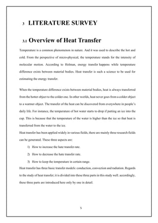
Figure 5. Convection heat transfer
Figure 5 has shown heat convection in a room. The air around the radiator is heated up by the
radiator and then moves to the cool region.
3.1.2.1 Newton’s law of cooling
The basic formula of calculating convective heat transfer rate is the Newton’s law of cooling.
The Newton’s law of cooling can be used to express the overall effect of convection [2]:
𝑞𝑞 = ℎ𝐴𝐴∆𝑇𝑇 (6)
Where
q is heat-transfer rate;
h is convection heat transfer coefficient, W/ (m2.k)
A is area, m2
△T is temperature difference between fluid and surface, K
As formula (6) showing above, convection heat transfer coefficient is one of the most important
parts of the formula. The main task of investigating the convection is to solve convection heat
transfer coefficient. Once the heat transfer coefficient has been found, the heat transfer rate can
be calculated. [2]
3.1.2.2 Overview of fluid mechanics.
A fluid can be classified based on the physical characteristics of flow fields. Figure 6 shows
one possible classification of flow.

21. 11
Newtonian fluid is defined as that the surface shear stress is directly proportional to rate of
deformation, which is expressed as:
𝜏𝜏𝑦𝑦𝑦𝑦 = 𝜇𝜇
𝛿𝛿𝛿𝛿
𝛿𝛿𝛿𝛿
(7)
Where
𝜏𝜏𝑦𝑦𝑦𝑦 is shear stress
μ is the dynamic viscosity
u is velocity
Viscous flows and Inviscid flows are both Newtonian fluids, the difference is that the viscosity
of inviscid flows are neglected. Accordingly, the fluid viscosity is assumed to be zero.
Laminar and Turbulent flow are classified based on the flow structure. The structure of
laminar flow is characterized by smooth motion layers. Being different with laminar flow, the
structure of the Turbulent flow is random.

22. 12
Internal and External flow. The main difference between them is if a flow is completely
bounded by solid surface.
Compressible and Incompressible Flows are termed on the basis of density variations.
Incompressible flow is termed as the density variations are negligible. In contrast, if the flows
in which variations in density are not negligible, it called compressible flows.
3.1.2.3 Convection Transfer Equation
Convection boundary layer
When a viscous Newtonian flow over a flat plate, the liquid velocity near the wall falls down
quickly, and then a thin layer is formed on the surface of the plate. This layer is called
boundary layer. Holman [4] also gave a clear concept that the boundary is described as the
observation of viscosity phenomena of the area of flow which derives from the leading edge
of the plate, both laminar and turbulent developed in this region. The Reynolds number,
which is the ratio for inertia forces to viscous forces, is used for distinguish the laminar
region and turbulent region in the boundary layer. The Reynolds number expressed as:
Rex = U∞ x/ v (7)
Where: -
ρ is the density of flow,
U∞ is free-stream velocity
v = μ/ρ is kinematic viscosity
x is distance from leading edge
A laminar region occurs when Rex ≤5 x 105.

23. 13
Figure 7-8 shows the velocity and thermal boundary layer, respectively. As Yang & Tao [2]
said that the heat transferred through this boundary layer. Based on these boundary layers, the
convection equation is derived to describe convective heat transfer problems with mathematical
formulation, the Continuity Equation, Momentum Equation and Energy Equation should be
applied. [2]
Continuity Equation on boundary layer
Conservation of mass is described as
[Net rate of mass flux out through the control surface]
+ [Rate of mass inside the control volume] = 0
For mass conservation in the two-dimensional velocity, the mass conservation is expressed as
𝜕𝜕𝜕𝜕𝜕𝜕
𝜕𝜕𝜕𝜕
+
𝜕𝜕𝜕𝜕𝜕𝜕
𝜕𝜕𝜕𝜕
= 0 (8)

24. 14
Where
𝜌𝜌 is density,
u and v are velocity
The equation (8) is also called continuity equation.
Momentum Equation on boundary layer
Within the unit time, the momentum balance for a control volume is given by:
[Rate of change of momentum inside the control volume] + [Net rate of flux of momentum
out through the control surface] = [Forces acting on the control volume]
The momentum equation in a two-dimensional velocity boundary layer is expressed as:
The x-momentum equation:
𝜌𝜌 �𝑢𝑢
𝜕𝜕𝜕𝜕
𝜕𝜕𝜕𝜕
+ 𝑣𝑣
𝜕𝜕𝜕𝜕
𝜕𝜕𝜕𝜕
� = −
𝜕𝜕𝜕𝜕
𝜕𝜕𝜕𝜕
+
𝜕𝜕
𝜕𝜕𝜕𝜕
�𝜇𝜇 �2
𝜕𝜕𝜕𝜕
𝜕𝜕𝜕𝜕
−
2
3
�
𝜕𝜕𝜕𝜕
𝜕𝜕𝜕𝜕
+
𝜕𝜕𝜕𝜕
𝜕𝜕𝜕𝜕
��� +
𝜕𝜕
𝜕𝜕𝜕𝜕
�𝜇𝜇 �
𝜕𝜕𝜕𝜕
𝜕𝜕𝜕𝜕
+
𝜕𝜕𝜕𝜕
𝜕𝜕𝜕𝜕
�� + 𝑋𝑋 (9)
The y-momentum equation:
𝜌𝜌 �𝑢𝑢
𝜕𝜕𝜕𝜕
𝜕𝜕𝜕𝜕
+ 𝑣𝑣
𝜕𝜕𝜕𝜕
𝜕𝜕𝑦𝑦
� = −
𝜕𝜕𝜕𝜕
𝜕𝜕𝜕𝜕
+
𝜕𝜕
𝜕𝜕𝜕𝜕
�𝜇𝜇 �2
𝜕𝜕𝜕𝜕
𝜕𝜕𝜕𝜕
−
2
3
�
𝜕𝜕𝜕𝜕
𝜕𝜕𝜕𝜕
+
𝜕𝜕𝜕𝜕
𝜕𝜕𝜕𝜕
��� +
𝜕𝜕
𝜕𝜕𝜕𝜕
�𝜇𝜇 �
𝜕𝜕𝜕𝜕
𝜕𝜕𝜕𝜕
+
𝜕𝜕𝜕𝜕
𝜕𝜕𝜕𝜕
�� + 𝑌𝑌 (10)
Where,
X and Y are the forces
p is the pressure
Formula (9) and (10) are also called Navier-Stokes equations.
Energy Equation on boundary layer:
As same as the description of energy equation in conduction section, the energy equation for
a two-dimensional boundary layer is
𝝆𝝆𝝆𝝆𝝆𝝆 �𝒖𝒖
𝝏𝝏𝝏𝝏
𝝏𝝏𝝏𝝏
+ 𝒗𝒗
𝝏𝝏𝝏𝝏
𝝏𝝏𝝏𝝏
� =
𝝏𝝏
𝝏𝝏𝝏𝝏
�𝒌𝒌
𝝏𝝏𝝏𝝏
𝝏𝝏𝝏𝝏
� +
𝝏𝝏
𝝏𝝏𝝏𝝏
�𝒌𝒌
𝝏𝝏𝝏𝝏
𝝏𝝏𝝏𝝏
� + 𝝁𝝁∅
�
�⃗ + 𝒒𝒒̇ (11)
Where,
∅
�
�⃗ is viscous dissipation.
The formula (8)-(11) are the partial differential equations of convection heat transfer. It

25. 15
is difficult to solve the equations if considering all of the terms, the simplified equations can
be derived by considering the boundary layer as incompressible, having constant properties,
negligible body forces and without energy generation.
3.1.2.4 The convection coefficients
According to Newton’s Law of cooling, once the convection heat transfer coefficient is known,
we can compute how much heat has been transferred between the flow and object. The
convection coefficients are influenced by a number of factors during the process of the heat
transfer, for instance, the density of the flow, the viscosity of the flow, the velocity of the flow
and so on. The analysis of convection heat transfer equation is about to obtain a formula for
convection heat transfer coefficient in different conditions. The formula below can be used for
computing the convention heat transfer coefficient of a flow over plate plane.
𝒉𝒉 = 𝟎𝟎. 𝟑𝟑𝟑𝟑𝟑𝟑
𝒌𝒌
𝒙𝒙
(𝑹𝑹𝑹𝑹𝒙𝒙)
𝟏𝟏
𝟐𝟐(𝑷𝑷𝑷𝑷)
𝟏𝟏
𝟑𝟑 (12)
Where
Rex is Reynolds Number,
Pr =
𝑣𝑣𝑣𝑣𝑐𝑐𝑝𝑝
𝑘𝑘
Prandtl Number
The equation (12) also can be written as:
𝑵𝑵𝒖𝒖𝒙𝒙 =
𝒉𝒉𝒙𝒙𝒙𝒙
𝒌𝒌
= 𝟎𝟎. 𝟑𝟑𝟑𝟑𝟑𝟑(𝑅𝑅𝑅𝑅𝑅𝑅)
𝟏𝟏
𝟐𝟐(𝒑𝒑𝒑𝒑)
𝟏𝟏
𝟑𝟑 (13)
Where Nux is called Nusselt Number
3.1.3 Radiation Heat Transfer
For conduction and convection heat transfer, the heat can only be transferred through a material
medium. Whereas, the radiation heat transfer can exist in vacuum. Energy transfer through
electromagnetic waves is called as radiation. And the thermal radiation is a radiation
propagated as a result of a temperature. Finally, radiation heat transfer is defined as ―heat
transfer by the emission of electromagnetic waves which carry energy away from the emitting
object.

26. 16
3.1.3.1 Properties of radiation
A radiant energy transmitted can be reflected, absorbed and transmitted when it strikes a
material surface. According to the Energy Balance Equation, the relationship of them can be
expressed as: [4]
𝜶𝜶 + 𝝆𝝆 + 𝝉𝝉 = 𝟏𝟏 (14)
where, 𝛼𝛼 is absorptivity, 𝜌𝜌 is reflectivity and 𝜏𝜏 is transmissivity.
Incident radiation Reflection
Transmitted
Figure 9. Effects of incident radiation
Figure 9 shows the effects of incident radiation. If a body absorbs total incident radiation, this
body is called Blackbody. Therefore, the absorptivity of blackbody is 1.
3.1.3.2 Stefan-Boltzmann law of thermal radiation
A concept of the emissive power was given by Holman [4] as ―the energy emitted by the
body per unit area and per unit time‖, it is marked with E. [4, p386]
The Stefan-Boltzmann law of thermal radiation describes a relationship between emissive
power of a blackbody and temperature. It shows as:
𝑬𝑬𝒃𝒃 = 𝝈𝝈𝑻𝑻𝟒𝟒
(15)
Where: -
Eb is the energy radiated per unit time and per unit area.
𝜎𝜎 is the Stefan-Boltzmann constant with value of 5.669 x 10-8 W/m2K4
T is temperature, K

27. 17
Equation (15) is called as the Stefan-Boltzmann law. Based on the law, it is known that a
subject’s emissive power increases as soon as the subject’s temperate rises.
The blackbody is an ideal body. Thus, when under the scenario of the same temperature, the
emissive power of the blackbody always has a stronger temperature degree than the actual
body. The ratio of the emissive power between the real body and blackbody at the same
temperature is called emissivity of the real body, which is [2, p365]:
𝜺𝜺 = 𝑬𝑬
𝑬𝑬𝒃𝒃
� (16)
Then the emissive power of a real body can be expressed as:
𝑬𝑬 = 𝜺𝜺𝑬𝑬𝒃𝒃 = 𝜺𝜺𝜺𝜺𝑻𝑻𝟒𝟒
(17)
The emissivity of a blackbody is 1.
3.1.3.3 Radiation Energy Exchange
Radiation Energy Exchange between blackbodies
To calculate the energy exchange between two blackbodies with surfaces Am and An, the
following expression would be applied
Q1-2 = EbmAmFmn – EbnAnFmn (18)
Where Fmn is the fraction of energy leaving surface m which reaches surfaces n.
Radiation Energy Exchange between non-blackbodies
Holman [4] has given definitions for two terms in order to calculate the radiation energy
exchange: Irradiation G and Radiosity J. Irradiation is ―the total radiation incident upon a
surface per unit time and per unit area [4, p410]‖ and Radiosity is ―total radiation which leaves
a surface per unit time and per unit area [4, p410]‖. As a result, the radiosity on a surface can
be calculated by the following formula, which has been mentioned by
𝑱𝑱 = 𝜺𝜺𝑬𝑬𝒃𝒃 + 𝝆𝝆𝝆𝝆 = 𝜺𝜺𝜺𝜺𝑻𝑻𝟒𝟒
+ 𝝆𝝆𝝆𝝆 (19)
Where
𝜀𝜀 is emissivity
Eb is the blackbody emissive power

28. 18
𝜌𝜌 is the reflectivity
𝜎𝜎 is the Stefan-Boltzmann constant
According to equation (18) and (19), an inferential reasoning formula (20) can be used for
calculating the radiation energy loss of an object in a large room.
𝒒𝒒 = 𝝈𝝈𝑨𝑨𝟏𝟏𝜺𝜺𝟏𝟏�𝑻𝑻𝟏𝟏
𝟒𝟒
− 𝑻𝑻𝟐𝟐
𝟒𝟒
� (20)
Where
A1 is the area of the object
𝛆𝛆𝟏𝟏 is the emissivity of the object
T1 is the temperature of the object
T2 is the temperature of the room
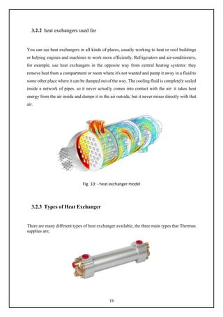
3.2 Heat Exchanger
heat exchanger is a device which transfers heat from one medium to another, a Hydraulic Oil Cooler
or example will remove heat from hot oil by using cold water or air. Alternatively, a Swimming Pool
Heat Exchanger uses hot water from a boiler or solar heated water circuit to heat the pool water. Heat
is transferred by conduction through the exchanger materials which separate the mediums being
used. A shell and tube heat exchanger pass fluids through and over tubes, where as an air-cooled heat
exchanger passes cool air through a core of fins to cool a liquid.
3.2.1 Working theory of Heat Exchanger
A heat exchanger works as a specialized device of helping the heat to transfer from the hot
fluid to the cold one. [14]. Heat exchanger not only exists in the aspect of engineering but also
happens in people’s life. Working as a heat exchanger, A heat exchanger is a device that
allows heat from a fluid (a liquid or a gas) to pass to a second fluid (another liquid or
gas) without the two fluids having to mix together or come into direct contact. If that's not
completely clear, consider this. In theory, we could get the heat from the gas jets just by
throwing cold water onto them, but then the flames would go out! The essential principle of a
heat exchanger is that it transfers the heat without transferring the fluid that carries the heat.

29. 19
3.2.2 heat exchangers used for
You can see heat exchangers in all kinds of places, usually working to heat or cool buildings
or helping engines and machines to work more efficiently. Refrigerators and air-conditioners,
for example, use heat exchangers in the opposite way from central heating systems: they
remove heat from a compartment or room where it's not wanted and pump it away in a fluid to
some other place where it can be dumped out of the way. The cooling fluid is completely sealed
inside a network of pipes, so it never actually comes into contact with the air: it takes heat
energy from the air inside and dumps it in the air outside, but it never mixes directly with that
air.
Fig. 10: - heat exchanger model
3.2.3 Types of Heat Exchanger
There are many different types of heat exchanger available, the three main types that Thermax
supplies are;

30. 20
 Shell and Tube: - Shell and Tube Heat Exchangers consist of a large number of small
tubes which are located within a cylindrical shell. The tubes are positioned into the
cylinder using a tube bundle or "tube stack" which can either have fixed tube plates
(permanently fixed to the body) or, in the case of Thermax Heat Exchangers a floating
tube stack which allows the tube bundle to expand and contract with varying heat
conditions as well as allowing the tube bundle to be easily removed for servicing and
maintenance.
 Plate type: - Plate Heat Exchangers operate in very much the same way as a shell and
tube heat exchanger, using a series of stacked plates rather than tubes. Plate heat
exchangers are usually brazed or gasketed depending on the application and fluids
being used. Their compact stainless-steel construction makes them an ideal choice for
use with refrigerants or in food and beverage processing.
 Air Cooled: - Air Cooled Heat Exchangers are commonly used in vehicles or other
mobile applications where no permanent cool water source is available. Thermax
designs and supplies combination cooling packs (or combi-coolers) which combine an
engine jacket water cooler, oil cooler and charge air cooler into a single unit reducing
space requirements and improving efficiency. Cool air is provided either by a fan or by
air flow caused by the movement of the vehicle.

31. 21
Chapter 4
4.1 COMSOL Multiphysics Software
Following with the major boost brought by computer technology, more and more computer
software has been widely developed and used in the arena of engineering. The usage of the
software can help engineers to solve problems efficiently. COMSOL Multiphysics is the
software, by using which, engineer can not only make drawings but also do physical analysis.
4.1.1 History
The COMSOL Group was founded by Mr. Svante Littmarck and Mr. Farhad [19] in Sweden
in 1986. It has now grown to United Kingdom, U.S.A, Finland and so on. Nowadays, The
COMSOL Multiphysics software has been widespread used in various domains of science
research and engineering calculation, for example, it was used in global numerical simulation.
COMSOL Multiphysics is a finite element analysis, solver and Simulation software package
for solving various physics and engineering applications. The first version of COMSOL
Multiphysics software was published in 1998 by COMSOL group and it was named as
Toolbox. At the beginning time, this software is only applied in the field of Structural
Mechanics. ―The COMSOL Multiphysics simulation environment facilitates all steps in the
modeling process —defining your geometry, specifying your physics meshing, solving and
then post-processing your results
4.1.2 Application areas
There are several application-specific modules in COMSOL Multiphysics. The most common
applications are
 AC/DC Module
 Acoustics Module
 CAD Import Module
 Chemical Engineering Module
 Earth Science Module
 Heat Transfer Module
 Material Library
In this thesis, only Heat Transfer Module will be introduced and used in order to solve the
relating problems of heat transfer.
4.1.3 Characteristics

32. 22
The spread usage of COMSOL Multiphysics in various domains largely depends on its
marked characteristics. These characteristics are
 It can be used to solve multi-physics problem
 The user can specify their own Partial Differential Equations
 Professional predefined modeling interfaces
 CAD models can be made directly
 CAD package can be added
 Exuberance of simulation capability
4.2 PROBLEM SOLVING PROCESS
4.2.1 COMSOL Multiphysics excels in solving systems of coupled
nonlinear PDEs that can include:
 Heat transfer
 Mass transfer through diffusion and convection
 Fluid dynamics
 Chemical reaction kinetics
 Varying material properties
The Multiphysics capabilities of COMSOL can fully couple and simultaneously model fluid
flow, mass and heat transport, and chemical reactions.
4.2.1.1 The modelling processes
The modelling process in COMSOL consists of six main steps: -
 Selecting the appropriate application mode in the Model Navigator.
 Drawing or importing the model geometry in the Draw Mode.
 Setting up the subdomain equations and boundary conditions in the Physics Mode.
 Meshing in the Mesh Mode.
 Solving in the Solve Mode.
 The model navigator
When starting COMSOL Multiphysics, you are greeted by the Model Navigator. Here you
begin the modeling process and control all program settings. It lets you select space

33. 23
dimension and application modes to begin working on a new model, open an existing model
you have already created, or open an entry in the Model Library. COMSOL Multiphysics
provides an integrated graphical user interface where you can build and solve models by
using predefined physics modes.
 Create Geometry
An important part of the modeling process is creating the geometry. The COMSOL
Multiphysics user interface contains a set of CAD tools for geometry modeling in 1D, 2D,
and 3D.
The CAD Import Module provides an interface for import of Parasolid, SAT (ACIS), STEP,
and IGES formats.
In combination with the programming tools, you can even use images and magnetic
resonance imaging (MRI) data to create a geometry.
 Modelling physics and equations: -
From the Physics menu you can specify all the physics and equations that define a model
including:
• Boundary and interface conditions
• Domain equations
• Material properties
• Initial conditions
 Creating mesh: -
When the geometry is complete and the parameters are defined, COMSOL Multiphysics
automatically meshes the geometry. However, you can take charge of the mesh-generation
process through a set of control parameters.
For a 2D geometry the mesh generator partitions the subdomains into triangular or quadrilateral
mesh elements.
Similarly, in 3D the mesh generator partitions the subdomains into tetrahedral, hexahedral, or
prism mesh elements.

34. 24
Solution
Here COMSOL Multiphysics comes with a suite of solvers for stationary, eigenvalue, and time-
dependent problems. For solving linear systems, the software features both direct and iterative
solvers. A range of preconditioners are available for the iterative solvers COMSOL
Setup solver defaults appropriate for the chosen application mode and automatically detects
linearity and symmetry in the model. A segregated solver provides efficient solution schemes
for large Multiphysics models, turbulence modeling, and other challenging applications.
 Post processing: -
For postprocessing, COMSOL provides tools for plotting and postprocessing any model
quantity or parameter:
 Surface plots
 Slice plots
 Iso surfaces
 Contour plots
 Arrow plots
 Streamline plots and particle tracing
 Cross-sectional plots
 Animations
 Data display and interpolation
 Integration on boundaries and subdomains.

35. 25
Chapter 5
Heat Exchanger model procedure
5.1 How to Model a Shell and Tube Heat Exchanger
Shell and tube heat exchangers are one of the most widely used type of heat exchanger in the
processing industries (65% of the market according to H. S. Lee’s book, Thermal Design)
and are commonly found in oil refineries, nuclear power plants, and other large-scale
chemical processes. Additionally, they can be found in many engines and are used to cool
hydraulic fluid and oil. There are a variety of different configurations for these heat
exchangers, but their basic concept can be designed through the modelling of several key
components. These components can then be modified depending on the heat exchanger’s
specific use, allowing this fundamental design to be utilized in a variety of different
application areas.
5.2 Simulating a Shell and Tube Heat Exchanger
Design
The concept used to design a shell and tube heat exchanger is examined by exploring the
working model of a straight, crossflow, one pass shell and tube heat exchanger. The
geometry of such a model is shown below
Figure 11: Geometry of the shell-and-tube heat exchanger.

36. 26
Geometry of a basic shell and tube heat exchanger. In this example, two fluids are passed
through the heat exchanger. The first fluid, in this case water, is passed through the tubes,
while the second fluid, air, circulates within the shell of the heat exchanger but outside of the
tubes. Both fluids have different starting temperatures when entering the heat exchanger,
however after circulating within the shell and tubes, the fluids are brought closer to an
equilibrium temperature.
A Shell and Tube heat exchanger is often found in refineries as well as other large-scale
plants. There are several design variations and operating conditions that impact the optimal
performance of such devices. For the purpose of this example, we will be analysing a straight,
crossflow, one pass tube heat exchanger, with water flowing through the tube side and air
flowing through the shell side. We will define the heat exchanger’s material as structural
steel and will assume a k-epsilon turbulence model for the flow of both the air and the water.
5.3 STEPS OF SIMULATING MODEL
5.3.1 First, to define the material, right-click on Materials and open the
Material browser. Under the Built-In tab, choose Air and add the
material to the model. Similarly, open the Material Browser and add
Liquid Water to the Model. Define the water material by using the
selection list and choosing Water domain. Once again, add a third
material by opening the material browser and adding Structural steel.
Define the walls of the heat exchanger as steel by choosing boundary
from the geometric entity list, then choosing walls from the selections
list.
5.3.2 To assign the flow boundaries of the model, we will add inlet and outlet
conditions for the water and air flows. Right-click on Non-isothermal
flow, then go to the turbulent flow tab and add a boundary condition
Inlet. From the boundary selections list, choose Inlet water. In the
velocity U0 field, enter the water velocity as u_water. Now, right-click
on Inlet 1 and rename it as Inlet water. Similarly, add an outlet by right-

37. 27
clicking on Non-Isothermal Flow and going to k-epsilon turbulent flow
and adding a boundary condition outlet. From the Boundary selection
list, choose Outlet water, and from the Boundary Condition list choose
normal stress. This implies that the total stress in the tangential
direction to the boundary as well as the pressure reference are set to
zero, allowing the fluid to flow without any impedance. Now rename
Outlet 1 as Outlet water. Right-click Non-isothermal flow and add
another k-epsilon turbulent inlet. From the Selections List, choose inlet
air and in the Velocity, section change air velocity U0 to u_air. Then
rename Inlet 2 as Inlet air. Again, right-click on Non-isothermal flow
and add a k-epsilon turbulent outlet. From the Selection List, choose
Outlet air and Normal Stress as the Boundary Condition. Rename
Outlet 2 as Outlet air.
5.3.3 Let’s add the symmetry conditions to the flow by right-clicking on
Non-isothermal flow and going to Turbulent Flow, k-epsilon and
choosing Symmetry flow. From the Boundaries Selection list, choose
Symmetry. Right-click Non-isothermal flow and under Turbulent
Flow, k-epsilon choose Interior wall. From the selection list, choose
Walls as the interior boundaries.
5.3.4 To define the heat transfer conditions, we will define temperatures at
the inlets, and the outflow at the outlets. Like the flow, we also must
define the symmetry conditions for the heat transfer. In addition, we
will use the highly conductive layer feature to account for the heat
conduction through the shell. Right-click on Non-isothermal flow, go
to Heat transfer and add a Temperature boundary. From the Boundary
Selections list, choose Inlet water. In the temperature field, type in
T_water, then rename Temperature 1 as Temperature water. Right-
click on Non-isothermal flow and under Heat transfer, add an Outflow.
From the Boundary Selections, list choose Outlet water, then rename
Outflow 1 as Outflow water.
5.3.5 Add another temperature boundary by right-clicking on Non-
isothermal flow. From the Boundary Selection list, choose Inlet air and

38. 28
in the Temperature field type T_air. Rename Temperature 2 as
Temperature air. Also add another Outflow boundary by right-clicking
on Non-isothermal flow. Change the boundary to Outlet air, then
rename Outflow 2 as Outflow air.
5.3.6 Now add a symmetry property to the heat transfer equations by right-
clicking on Non-isothermal flow and under Heat transfer choose
Symmetry, heat. From the Boundary Selection list choose Symmetry.
Right-click on Non-isothermal flow and go to Heat Transfer and
choose the boundary condition Highly Conductive Layer. From the
Selections list choose Walls and change the layer thickness to 5
millimetres.
5.3.7 Now we will define modelling coupling operators in order to evaluate
the equivalent heat transfer coefficient. Right click on Definitions and
go to model couplings and choose average. Change the geometric
entity to boundary and from the boundary list choose Inlet water.
Right-click average 1 and rename it as Average 1: Inlet water.
Similarly, add another average operator by right-clicking on
Definitions. Choose boundary as the geometric entity and from the
selections list choose Inlet air. Rename average 2 as Average 2: Inlet
air. Now, right-click on definition, go to model couplings and select
Integration. Choose Boundary as the geometric entity and select
Water-air walls as the Boundary. Rename integration 1 as Integration
1: Water-air walls.
5.3.8 Given the complexity of this model, the computation time can greatly
vary depending on the mesh size defined by the user. It is important to
balance between accuracy and computational cost in order to ensure
the most accurate solution in a timely manner. For the purpose of this
example, we will define a modified physics induced extremely coarse
mesh in order to obtain a relatively quickly solution while remaining
accurate.

39. 29
5.3.9 In the mesh settings window, change the element size to extremely
coarse, then right-click Mesh 1 and select edit physics induced
sequence. Click on Free tetrahedral 1, then under the scale geometry
section set the x-direction scale field to 0.5. Then under the Boundary
layer 1 node select Boundary layer properties 1 and define the number
of boundaries as 3, then click build all. Once the mesh is built, you are
ready to compute Study 1.
5.3.10 Please note that it takes about 3 hours to compute the model with an
average computer containing 12 Gigabytes of free memory. Depending
on the computational power of your machine, this time may vary.
5.3.11 Once the results are calculated, expand the Wall resolution node and
click on Surface 1. In the expression section, click replace expression
then choose Non-isothermal flow, Upside, and select Wall lift off.
Click plot to see the upside wall lift-off for the tubes. From this graph
you can see where the most critical areas in terms of mesh resolution
are located. Typically, an acceptable wall lift-off should remain under
10% of the tube radius. In this plot you can see that most of the wall
lift-off remains under the 10%, which makes this mesh resolution
sufficiently refined for the purpose of this example.
5.3.12 Now that we have validated the model, let us analyse the temperature
distribution along all the wall boundaries. Under the Data Sets node
click Surface 1. From the selection list, choose Walls as the boundary.
Under results expand Temperature and click on Surface 1, then change
the default temperature unit to degC. Click plot to view the temperature
distribution along the new surface.
5.3.13 In order to create a 3D streamline view illustrating the velocity and the
temperature, we will mirror the solution obtained by the original half
heat exchanger geometry. Right-click on data sets, go to more data sets
and add a Mirror 3D. From the plane list, choose zx-planes as the plane
of symmetry. Right-click on results and add a 3D Plot group. From the
data set list, choose Mirror 3D1. Right-click on 3D Plot Group 4 and

40. 30
add a streamline. In the points edit field under the streamline
positioning section, type in 100 to define the number of streamlines in
the plot. Then define the line type as tube in order to make the
colouring of the velocity field more visible. Right-click on Streamline
1 and choose Colour Expression. From the color table list choose
Thermal. Right-click on 3D Plot Group 4 and rename it as Velocity,
streamline.
5.3.14 This figure illustrates the air flow as well as the water flow through the
heat exchanger. The largely different heat capacities between the
air and the water are clearly portrayed in this plot as the temperature
of the air changes much more drastically than that of the water when it
flows through the heat exchanger.
5.3.15 Now, right-click on Derived Values, and add a Global evaluation.
Using the integration and average coupling operators defined earlier,
type in the following expression to define the heat transfer coefficient.
Here you can see the global expressions embedded in the terms for: the
power, the area, the inlet hot temperature and the inlet cold
temperature. Click evaluate to solve for the heat exchanger’s overall
heat transfer coefficient. Right-click on Global Evaluations 1 and
rename it as Heat Transfer coefficient.
5.3.16 Let us now analyse the average water inlet pressure as well as the
average air inlet pressure. Right-click derived values and go to average
then select Surface average. From the selection list choose Inlet water
and, in the expression, field enter p then click on the evaluate button to
see the average inlet water pressure. This result is equivalent to the
water pressure drop across the heat exchanger, as the outlet water
pressure is almost zero. Right-click on Surface Average 1 and rename
it as Inlet Pressure, Water. Right-click on Derived Values and add
another Surface Average. From the boundary selection list, choose
Inlet air and in the expression field, type in P. Now, click the evaluate
button to see the average inlet air pressure. Similarly, this value is

41. 31
equivalent to the air pressure drop across the heat exchanger. Right-
click on Surface Average 2 and rename it as Inlet Pressure, Air.
5.4 Model Definition
The concept used to design a shell-and-tube heat exchanger is examined by exploring the
working model of a straight, crossflow, one pass shell-and-tube heat exchanger. The
geometry of such a model is shown in below
Figure 12: Geometry of the shell-and-tube heat exchanger.
The heat exchanger is made of structural steel. In this example, two fluids pass through the heat
exchanger. The first fluid, in this case water, flows through the tubes, while the second fluid,
air, circulates within the shell of the heat exchanger but outside of the tubes.
Both fluids have different starting temperatures when entering the heat exchanger, however,
after circulating within it, the fluids are brought closer to an equilibrium temperature. The
baffles introduce some crossflow to the air and such increasing the area of heat exchange.
Another advantage is that baffles reduce vibration due to the fluid motion. This model uses the
No isothermal Flow predefined Multiphysics coupling configured with the k- turbulence

42. 32
model. It takes advantage of symmetries to model only one half of the heat exchanger, thereby
reducing model size and computational costs.
5.5 BOUNDARY CONDITION
All heat exchanger walls including the baffles are modelled as shells in 3D. This requires
special boundary conditions for the flow and heat transport equations.
The interior wall boundary condition for the flow separates the fluids from each other and
is also used to describe the baffles. On both sides, it applies the wall functions needed for
simulating walls with the k- turbulence model.
To account for the in-plane heat flux in the shell, the Thin Layer boundary condition is
applied. This boundary condition simulates heat transfer in thin shell structures. Here, the
shell is supposed made of steel and with a 5 mm thickness. beside the symmetry plane, all
remaining exterior boundaries are thermally insulated walls.
Figure13: Temperature at the heat exchanger boundaries

43. 33
5.6 Results and Discussion
An important criterion for estimating the accuracy of a turbulence model is the wall resolution.
Hence, COMSOL Multiphysics creates a plot of the wall resolution by default. The value for
δw
+
has must be 11.06, which corresponds to the distance from the wall where the logarithmic
layer meets the viscous sublayer. Furthermore, the wall lift-off δw has to be small compared to
the dimension of the geometry. On interior walls you have δw for the upside and downside of
the wall. To visualize the upside and downside directions, use an arrow surface plot with the
components unx, uny, and unz for the up direction and dnx, dny, and dnz for the down direction.
Figure 2 shows the upside wall lift-off. This is the wall lift-off inside the tubes where the
probably most critical area in terms of mesh resolution is located. It is about 10% of the tube
radius, which is sufficient.
Figure 14: Wall lift-off for the tubes.

44. 34
The tube side velocity shows a uniform distribution in the tubes. Before water enters the tubes,
recirculation zones are present. The streamline color represent the temperature and you can see
that the temperatures at both outlets are close to each other. Figure 4 shows the temperature
distribution on the heat exchanger
Figure 15: Velocity streamlines.
There are several quantities that describe the characteristics and effectiveness of a heat
exchanger. One is the equivalent heat transfer coefficient given by
heq =
p
A(𝑇𝑇hot – 𝑇𝑇cold)

45. 35
where P is the total exchanged power and A is the surface area through which P flows. In
this model the value of overall heat transfer coefficient is 5.5 W/(m2·K).
fig. No.: -16 over all heat transfer coefficient
 The pressure drop is about 38.5 Pa on the tube side
Fig. No: -17 pressure drop tube side

46. 36
 Pressure Drop across shell side13 Pa on the shell side
Fig.no: - 18 pressure drop across shell side

47. 37
CONCLUSION
In this study, three basic questions regarding conduction, convection, and radiation are solved
successfully. As a foundation, the part of theoretical methods benefits on analysing and solving.
By this means, we understand how to analyse and to solve the problems on heat transfer.
Furthermore, we apply COMSOL Multiphysics software to solve problem. Comparing the
results from the theoretical method with COMSOL Multiphysics software, it has been proved
that COMSOL Multiphysics software can offer accurate analysis. Meanwhile, it is a very
efficient tool for solving heat transfer problem, especially for those completed problems.
Based upon the simulation of the heat transfer process of Heat Exchanger. Through the
simulation on stainless steel Heat Exchanger with different thickness.

48. 38
Reference
i. https://www.comsol.co.in/model/shell-and-tube-heat-exchanger-12685
ii. The Finite Element Method: Basic Concepts and Applications with MATLAB,
MAPLE, and COMSOL, Third Edition
iii. https://wiki2.org/en/COMSOL_Multiphysics
iv. http://hyperphysics.phy-astr.gsu.edu/hbase/thermo/heatra.html
v. https://www.comsol.com/
vi. https://www.comsol.com/video/shell-tube-heat-exchanger-model-tutorial
vii. http://hyperphysics.phy-astr.gsu.edu/hbase/thermo/stefan.html
viii. https://www.comsol.com/model/shell-and-tube-heat-exchanger-12685
ix.