Final statistical treatment data

Semester IV S.Y.B.Sc. Paper III Unit III
1
Statistical Treatment of Analytical Data II
Nature of Indeterminate Error:
Indeterminate errors are those whose causes cannot be easily located and they do not have
definite values. These errors are of fluctuating a random type and therefore also called as
random errors are incorrigible error.
Indeterminate errors arises due to unknown uncertainties in measurements. When more
elaborate procedure and more steps involved there is higher chances of introducing
indeterminate errors.
For example, Gravimetric estimation. The net effect of indeterminate errors is to produce a
white divergence in numerical values of measurement made.
Statistical methods of analysis are used to study effect of indeterminate errors on the final
results.
The True and Acceptable Value of a Results Analysis
True value: In absence of systematic error, the population mean (µ) obtained for large
number of replicates measurements represents the true value for measured quantity.
Acceptable value of measurement:
In actual practice, it is not possible to estimate the true value for given set of measurements.
However, an acceptable value for a given measurement can be easily calculated by using
arithmetic mean. When N is small the mean 𝑥
̅differ from µ but if N as number of observation
is more than 30 then µ is not differ than 𝑥̅.
Numerically, the difference between true value and measured value is represented in terms
of absolute error and relative error.
Absolute error:
It is defined as numerical difference between measured value Xi and the accepted value or
true value Xt.
Absolute Error = 𝑋𝑖 – 𝑋𝑡
Relative error:
It is ratio of the absolute error to true value.
𝑅𝑒𝑙𝑎𝑡𝑖𝑣𝑒 𝐸𝑟𝑟𝑜𝑟 =
𝑋𝑖 – 𝑋𝑡
𝑋𝑡
(Numericals)

2
Measure of Central Tendency and Dispersion:
When repeated measurements carried out for the same sample which results in formation of
set. This set of measurement will have two characteristic one is central tendency and other is
dispersion.
A) Measure of Central Tendency:
Central tendency is measured by mean, mode and median.
i. Arithmetic Mean: 𝑥̅
It is the average value for given set of observation.
Since it is an average, the mean may not be an observation that is actually of
obtained.
𝑥̅ =
𝑥1 + 𝑥2+𝑥3 + ⋯ + 𝑥𝑛
𝑛
Where,
x1, x2, x3are individual observations
n, number of observations
Two drawbacks-
1. Since it is an average, the mean may not be an observation that is actually
obtained.
2. It is readily affected by the extreme values.
ii. Median: 𝒎
̅
When the observations are arranged in ascending order magnitude wise, the
central value, if the observations are odd in number and the mean of the central
pair when they are even in number is known as median.
e.g. 10.2, 10.4, 10.8, 11.0, 11.2 (Median is 10.8)
10.2, 10.4, 10.8, 11.0, 11.2, 11.4
=
10.8+11.0
2
= 10.9 is median
𝑥̅ =
∑ 𝑥𝑖
𝑛
𝑖=1
𝑛

3
iii. Mode:
It is defined as the observation that repeats itself maximum number of
times.
If the observations are not repeated the set will have no mode.
On the other hand, if the observations are repeated themselves for same
maximum of times then all that observations will become mode.
(Numericals)
B) Measure of Dispersion:
Different measures of dispersions are available. They can be broadly classified as the
measures of dispersion for a single observation and measures of dispersion for a set of
observations.
Measures of Dispersion for a single Observation
i. Absolute Deviation
It is defined as the difference between an observation and the mean.
𝒅𝟏 = 𝒙𝟏 − 𝒙
̅
ii. Relative Deviation
The ratio of the deviation to the mean is known as relative deviation.
𝑅. 𝐷. =
𝐷𝑒𝑣𝑖𝑎𝑡𝑖𝑜𝑛
𝑀𝑒𝑎𝑛
𝑅. 𝐷. =
𝒙𝟏 − 𝒙
̅
𝑥̅
iii. Average Deviation
It is defined as the arithmetic mean of all the deviations when only the
numerical values are considered.
𝑑̅ =
𝑑1 + 𝑑2+𝑑3 + ⋯ + 𝑑𝑛
𝑛
𝑑̅ =
∑ 𝑑𝑖
𝑛

4
iv. Relative Average Deviation
It is defined as the ratio of the average deviation to the mean of the set of
observations.
𝑅. 𝐴. 𝐷. =
𝑑̅
𝑥
̅
It is expressed, usually, as pph or ppt
R. A. D. in parts per hundred =
𝑑̅
𝑥
̅
𝑋 100
R. A. D. in parts per thousand =
𝑑̅
𝑥
̅
𝑋 1000
Measures of Dispersion for a Set of Observations
i. Range
It is defined as the difference between the maximum and the minimum
value.
Range = 𝑥𝑚𝑎𝑥 − 𝑥𝑚𝑖𝑛
ii. Standard Deviation
It is defined as the square root of the mean of the square of the individual
deviations.
𝑆 = √
∑(𝑥1 − 𝑥̅)2
𝑁 − 1
Where N < 20
 = √
∑(𝑥1 − 𝑥̅)2
𝑁
Where N > 20
 = Population standard deviation
iii. Variance
Variance is defined as square of standard deviation.
Variance = S2
iv. Coefficient of Variation
Coefficient of variation is defined as the ratio of standard deviation to the
mean and is expressed as percentage.
𝐶. 𝑂. 𝑉. =
𝑆
𝑋
̅ X 100
(Numericals)

5
Distribution of Random Errors:
Indeterminate errors or Random errors arise as a consequence of small unknown uncertainty.
This error cannot be eliminated from measurement and at the same time they cannot be
ignored. Apart from personal random errors, some random errors may also be introduced in
measurements due to errors in the methods itself. This may be due to increase in Chemicals
or irregular variation of room temperature.
The task of analytical chemist to make a random error as small as possible. Hence the
distribution for random errors that is like to move the value in either direction is called as the
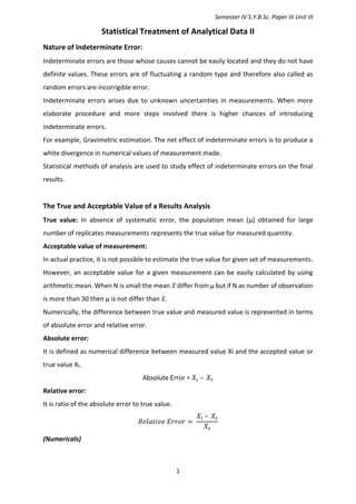
normal or Gaussian distribution. Such a distribution is characterized by two parameters, the
population mean μ and population standard deviation σ.
Gaussian Distribution Curve
For a large number of replicate measurements readings free of determinant error, the results
will generally be symmetrical distributed around the mean. By determining the relative
frequency of occurrence of a reading and plotting the values for different results, the curve
obtained is known as the normal distribution curve.
The equation of the curve is
y =
1
𝜎√2𝜋
exp − [
(𝑋𝑖 − 𝜇) 2
2𝜎2
]
Where,
y = the relative frequency of occurrence for given set of observation
xi = the value of corresponding observation of the set
μ = the mean of population of Universe with infinite number of observations
σ = standard deviation for the population comprising infinite number of observations.
The equation is the Gauss-Laplace equation and hence the distribution is also called as
Gaussian distribution curve or the normal error curve.

6
Graphical presentation of the curve
The curve can be presented in three different ways
Method 1- y-axis is the relative frequency of occurrence -y
x-axis the observation xi
xi
Method 2 - y axis the relative frequency of occurrence -y
x-axis xi-μ -deviation from the population mean
xi- μ
Method 3- y-axis the relative frequency of occurrence-y
x-axis population standard deviation-σ
σ
µ
µ
µ
relative frequency
of occurrence
relative frequency
of occurrence
relative
frequency of
occurrence

7
Characteristics of Gaussian Distribution
• The curve is symmetrical about the central value that is population mean
• As the magnitude of the deviation of either sign increases, the probability of its
occurrence decreases.
• The total area under the curve, covering all the possible values of xi from- to + will thus
represent the population.
• Every observation, irrespective of its magnitude has a definite probability of occurrence
Confidence Limits and Confidence Interval:
Any set of observations have two properties. One is the central tendency and the second is
dispersion or spread. Mean 𝑥̅ is a measure of central tendency and standard deviation S is
measure of spread or dispersion.
Consider set of observations which have infinite number of observations. This is known as
population or universe.
For this set also, the measures of central tendency will be the mean and measure of dispersion
will be the standard deviation. The mean for the set of infinite number of observations is
called as population mean  and the standard deviation for the set of in for infinite number
of observation is called as the population standard deviation denoted as .
As the number of observations in the given set increases, the difference between𝑥
̅ and  as
well as that between S and , will get reduced.
In actual practice the difference between S and  beyond a certain number (more than 20
observations) is negligible or almost reduced to zero. Thus, when the number of observations
exceed twenty the standard deviation S can be taken to be same as the population standard
deviation .
Similarly, as the number of observations increase, the difference 𝑥
̅ and  decrease. However,
even with a very large number of observations, the difference never becomes very very small.
Thus, it is never possible to substitute 𝑥
̅ for  even with a very large number of observations.
Hence it becomes necessary to get an estimate of  in terms of arithmetic mean 𝑥
̅.
However, it is possible to state the limits or the range on the either side of arithmetic mean𝑥̅
and there is a 50% or 90% or 99% or any other chance or probability that the population mean
µ lies in a particular range.
Limits are called as confidence limit.

8
Confidence interval:
The interval so defined by confidence limits around the arithmetic mean 𝑥̅ is it defined as
confidence interval.
There are different ways of obtaining confidence limit and confidence interval.
1. Using Student’s t: It was first introduced by Gosset.
Confidence limits = ±
𝑡𝑠
√𝑛
Confidence Interval = 𝑥
̅±
𝑡𝑠
√𝑛
So that the interval defined as = 𝑥
̅ -
𝑡𝑠
√𝑛
to 𝑥
̅̅̅ +
𝑡𝑠
√𝑛
Where,
t = student’s t is a statistical parameter
𝑥̅ = mean
𝑛 = No. of observations
Degree of Freedom = n-1, where ‘n’ is No. of observations
t values for various confidence levels
Degree of
freedom
80% 90% 95% 98% 99% 99.9%
1
2
3
4
5
6
7
8
9
10
11
12
13
14
15
2. Using Range: confidence limits can also be defined in terms of range for the given set
of observations.
Confidence limits = ± CnR
Confidence Interval = 𝑥̅ + CnR to 𝑥̅ - CnR
Where, Cn is another statistical parameter.
Values for Cn

9
Degree of freedom 95% 99%
2 6.35 31.8
3 1.30 3.01
4 0.72 1.32
5 0.51 0.84
6 0.40 0.63
7 0.33 0.51
8 0.29 0.43
9 0.26 0.37
10 0.23 0.33
11 0.21 0.30
12 0.19 0.27
3. Using Population Standard deviation: This method is applicable only when the
number of observations is very large.
Confidence limits = ±
𝑧𝑠
√𝑛
Confidence Interval = 𝑥
̅±
𝑧𝑠
√𝑛
So that the interval defined as = 𝑥̅ -
𝑧𝑠
√𝑛
to 𝑥
̅̅̅ +
𝑧𝑠
√𝑛
Criteria for Rejection of Doubtful Result
In replicate measurements, few measurements have some deviation from rest of the set of
measurements and therefore such values are rejected. This becomes dilemma for the
scientist to reject or not to reject the doubtful value. If such doubtful values not rejected then
this will give rise an error in the mean while rejection may lead to discarding of rightful values.
Hence for the rejection of doubtful values some rule or test applied
2.5d Rule:
1. Discarding the doubtful observation, obtain the mean of the remaining observations.
2. With the help of new mean obtained in step (1), calculate the average deviation of the
set.
3. Calculate the deviation of the doubtful observation from the new mean.
4. If the deviation of the doubtful observation is equal to or greater than 2.5 times average
deviation, then reject doubtful observations.

10
4.0 d Rule:
1. In the case of 4.0d rule steps involved from (1) to (3) are identical. Only the last step is
different.
2. In the deviation of doubtful observation is equal to or greater than 4.0 times average
deviation, then reject doubtful observations.
(Numericals)
The Q-Test:
Dean and Dixon applied the Q-Test for first time. The test has statistical basis. When the Q-
Test delivers the verdict in favour of the rejection of a result the result is indeed subject to
special error. The drawback of the test is, it rejects the result only when the deviation is large.
Thus, with an error of small magnitude, that may produce a small deviation. The result may
be retained by the Q-Test.
The steps involved in the application of the Q-Test as follows-
1. Arrange the observations in the ascending order of magnitude.
2. Calculate the range of result.
3. Find the difference between the doubtful observation and its nearest neighbour.
4. Calculate the Rejection Quotient Q,by dividing the difference obtained in step (3) with
the range obtained in step (2).
5. From the table of Q- values, obtain the appropriate value of Q for a given probability
level and for a given number of observations.
6. If Qcal>Qtabulated then the doubtful observation is to be rejected otherwise it is to be
retained.
Rejection Quotient Q for 90% Probability Level
No. of Measurements Q at 90% of probability
3 0.94
4 0.76
5 0.64
6 0.56
7 0.51
8 0.47
9 0.44
10 0.41
11 0.39
12 0.37
(Numericals)

11
Testing for Significance:
Null Hypothesis
When a sample is analysed by more than one method, more than one set of results for the
same sample may be available. For these sets statistics cannot provide any information as
which mean of the set is more accurate. But we can certainly have obtained information as
to whether the difference in the two means for the two sets implies in population mean
(statistically) or only a numerical difference.
In short statistics can provide the information, whether the two means differ statistically or
they are only numerically different.
If the two means differ statistically, then obviously their population means are also different.
The test used by the statistics to decide whether the two means differ statistically or not is
known as the Null Hypothesis.
The steps involved are as follows:
1. Using the following expression calculate the value of the expression is:
𝑡𝑐𝑎𝑙𝑐 =
|𝑥̅1 − 𝑥̅2|
𝑠
√
𝑛1𝑛2
𝑛1 + 𝑛2
𝑥̅1- mean of the observations of set I.
𝑥̅2 – Mean of the observations of set II.
n1- the number of observations of the set I.
n2- the number of observations of set II.
s- Standard deviation. As the two standard deviations are not different than any
one value can be used or s is calculated as follows:
𝑠 = √
∑(𝑥𝑖 − 𝑥̅1 )2 + ∑(𝑥𝑖 − 𝑥̅2 )2
𝑛1 + 𝑛2 − 2
2. Compare the tcal value with the tabulated value of t for (n1 + n2 -2) no. of degrees of
freedom and for the given probability level.
Result: - In the comparison only two possibilities will arise.
A) tcal<ttab. This means that the null hypothesis is valid and the two means do not differ
statistically but only numerically.
B) If tcal>ttab. Then the null hypothesis is not valid and the two means arenot only
numerically different they are even statistically different.

12
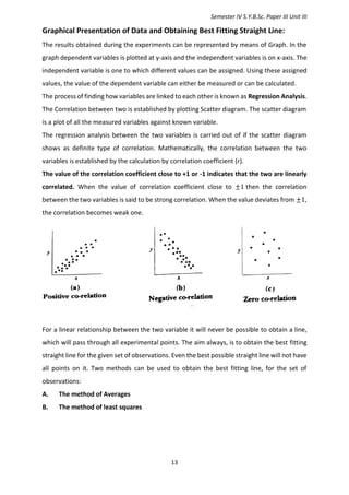
The variance Ratio Test- F Test:
The variance ratio test is used to find out whether the two standard deviations obtained for
the two sets of the observations of the same sample differ only numerically or statically.
Variance is defined as the square of the standard deviation. The ratio of the two variances for
the two sets of observations are considered in this test and hence the name is Variance Ratio
Test. The steps involved in the calculation of the variance ratio test are as follows:
i) Calculate the standard deviations S1 and S2 for the two sets of observations.
ii) Calculate the variance ratio which is known as F in such a way that the ratio is greater
than one. This is done by placing the larger standard deviation in the numerator.
𝐹𝑐𝑎𝑙 =
𝑠1
2
𝑠2
2 𝑠1 > 𝑠2
iii) From the table of F values [refer to table] for the given number of observations and
for the given probability level, obtain the appropriate value of F.
Result: There are only two possibilities.
1) Fcal<Ftab: In this case, the two standard deviations are not statistically different but
only numerically different.
2) Fcal>Ftab: In this case, the two standard deviations are not only differing
numerically but statistically as well
Tabulated values of the Statistical Parameter F
(n-1) for
smaller s2
n-1 for larger S2
1 2 3 4 5
1 161 200 216 225 230
2 18.51 19 19.16 19.25 19.30
3 10.13 9.55 9.28 9.12 9.01
4 7.71 6.94 6.59 6.39 6.26
5 6.61 5.79 5.41 5.19 5.05
6 5.99 5.14 4.76 4.53 4.34
7 5.59 4.74 4.35 4.12 3.47
8 5.32 4.46 4.07 3.84 3.69
9 5.12 4.26 3.86 3.63 3.48
10 4.96 4.10 3.71 3.48 3.33
(Numericals)

13
Graphical Presentation of Data and Obtaining Best Fitting Straight Line:
The results obtained during the experiments can be represented by means of Graph. In the
graph dependent variables is plotted at y-axis and the independent variables is on x-axis. The
independent variable is one to which different values can be assigned. Using these assigned
values, the value of the dependent variable can either be measured or can be calculated.
The process of finding how variables are linked to each other is known as Regression Analysis.
The Correlation between two is established by plotting Scatter diagram. The scatter diagram
is a plot of all the measured variables against known variable.
The regression analysis between the two variables is carried out of if the scatter diagram
shows as definite type of correlation. Mathematically, the correlation between the two
variables is established by the calculation by correlation coefficient (r).
The value of the correlation coefficient close to +1 or -1 indicates that the two are linearly
correlated. When the value of correlation coefficient close to ±1 then the correlation
between the two variables is said to be strong correlation. When the value deviates from ±1,
the correlation becomes weak one.
For a linear relationship between the two variable it will never be possible to obtain a line,
which will pass through all experimental points. The aim always, is to obtain the best fitting
straight line for the given set of observations. Even the best possible straight line will not have
all points on it. Two methods can be used to obtain the best fitting line, for the set of
observations:
A. The method of Averages
B. The method of least squares

14
A. The Method of Average:
The best fitting line for a given set of observation is that line for which the sum of the
deviations of all the points from the best fitting line is equal to zero.
To obtain a best fitting line the value of slope is fixed. This can be done in such a way
that the sum of deviations of all the points from straight line is equal to zero.
∑ 𝑑𝑖 = 0
if y is the value obtained for given value of x then ycal is the value of y for the same value
of x.
∑ 𝑦 − 𝑦𝑐𝑎𝑙 = 0
Case I: Line passing from origin
From the equation of line passing from origin
y = mx
But, ycal = mx
∑ 𝑦 − 𝑦𝑐𝑎𝑙 = 0
∑ 𝑦 − 𝑚𝑥 = 0
∑ 𝑦 − ∑ 𝑚𝑥 = 0
∑ 𝑦 = ∑ 𝑚𝑥
𝑚 =
∑ 𝑦
∑ 𝑥
From the value of ‘m’ equation of best fitting line is obtained.
Case II: Line not passing from origin
From the equation of line not passing from origin
y = mx + c
But, ycal = mx + c
∑ 𝑦 − 𝑦𝑐𝑎𝑙 = 0
∑ 𝑦 − (𝑚𝑥 + 𝑐) = 0
∑ 𝑦 − ∑ 𝑚𝑥 − ∑ 𝑐 = 0

15
∑ 𝑦 = ∑ 𝑚𝑥 + ∑ 𝑐
∑ 𝑦 = 𝑚 ∑ 𝑥 + ∑ 𝑐
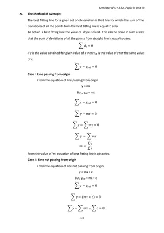
From the value of m and c equation of best fitting line is obtained.
B. The Method of Least Square:
In this method for the best fitting line sum of square deviation of all points from line is
minimum (equal to zero).
∑(𝑦 − 𝑦𝑐𝑎𝑙)2
= 0
Case I: Line passing from origin
From the equation of line passing from origin
y = mx
But, ycal = mx
∑(𝑦 − 𝑚𝑥)2
= 0
By differentiating,
𝑑
𝑑𝑚
∑(𝑦 − 𝑚𝑥)2
= 0(
𝑑
𝑑𝑚
𝑎𝑠 𝑚 𝑖𝑠 𝑣𝑎𝑟𝑖𝑎𝑏𝑙𝑒)
∑
𝑑
𝑑𝑚
(𝑦 − 𝑚𝑥)2
= 0
∑ 2 (𝑦 − 𝑚𝑥)
𝑑
𝑑𝑚
(𝑦 − 𝑚𝑥) = 0
2 ∑(𝑦 − 𝑚𝑥) [(
𝑑𝑦
𝑑𝑚
) − (𝑥
𝑑𝑚
𝑑𝑚
)] = 0
2 ∑(𝑦 − 𝑚𝑥)(0 − 𝑥) = 0
2 ∑ −𝑥𝑦 + 𝑚𝑥2
= 0
∑(−𝑥𝑦) + ∑(𝑚𝑥2
) = 0
𝑚 ∑ 𝑥2
= ∑ 𝑥𝑦
𝑚 =
∑ 𝑥𝑦
∑ 𝑥2
From the value of ‘m’ equation of best fitting line is obtained.

16
Case II: Line not passing from origin
From the equation of line not passing from origin
y = mx + c
But, ycal = mx + c
∑(𝑦 − 𝑦𝑐𝑎𝑙)2
= 0
∑(𝑦 − (𝑚𝑥 + 𝑐))2
= 0
∑(𝑦 − 𝑚𝑥 − 𝑐)2
= 0
By differentiating,
Here ‘m’ and ‘c’ both are variable
𝑑
𝑑𝑚
∑(𝑦 − 𝑚𝑥 − 𝑐)2
= 0
as well as
𝑑
𝑑𝑐
∑(𝑦 − 𝑚𝑥 − 𝑐)2
= 0
i)
𝑑
𝑑𝑚
∑(𝑦 − 𝑚𝑥 − 𝑐)2
= 0
∑ 2 (𝑦 − 𝑚𝑥 − 𝑐)
𝑑
𝑑𝑚
(𝑦 − 𝑚𝑥 − 𝑐) = 0
2 ∑(𝑦 − 𝑚𝑥 − 𝑐) [(
𝑑𝑦
𝑑𝑚
) − (𝑥
𝑑𝑚
𝑑𝑚
) − (
𝑑𝑐
𝑑𝑚
)] = 0
2 ∑(𝑦 − 𝑚𝑥 − 𝑐)[0 − (𝑥) − 0] = 0
∑(𝑦 − 𝑚𝑥 − 𝑐)( − 𝑥) = 0
∑ −𝑥𝑦 + 𝑚𝑥2
+ 𝑥𝑐 = 0
∑ 𝑥𝑦 = 𝑚 ∑ 𝑥2
+ 𝑐 ∑ 𝑥 ---------------- A

17
ii.
𝑑
𝑑𝑐
∑(𝑦 − 𝑚𝑥 − 𝑐)2
= 0
∑ 2 (𝑦 − 𝑚𝑥 − 𝑐)
𝑑
𝑑𝑐
(𝑦 − 𝑚𝑥 − 𝑐) = 0
2 ∑(𝑦 − 𝑚𝑥 − 𝑐) [(
𝑑𝑦
𝑑𝑐
) − (𝑥
𝑑𝑚
𝑑𝑐
) − (
𝑑𝑐
𝑑𝑐
)] = 0
2 ∑(𝑦 − 𝑚𝑥 − 𝑐)[0 − 0 − 1] = 0
∑(𝑦 − 𝑚𝑥 − 𝑐) − (1) = 0
∑ −(𝑦 − 𝑚𝑥 − 𝑐) = 0
− ∑ 𝑦 + ∑ 𝑚𝑥 + ∑ 𝑐 = 0
∑ 𝑦 = 𝑚 ∑ 𝑥 + ∑ 𝑐 ---------------- B
(Numericals)

Final statistical treatment data

More Related Content

What's hot

Similar to Final statistical treatment data

More from JLoknathDora

Recently uploaded

Final statistical treatment data