Department of ElectricalEngineering
Introduction
OutLine
In the previous class we have introduce FIR and IIR filters, We are
now in a position to consider the various approaches to their
design. The two types of filter, FIR and IIR, have very different
design methods and so will be considered separately.
In this class we will focus on the techniques used to design IIR or
recursive filters. We begin with a very brief resume of filter
essentials.
3.
Department of ElectricalEngineering
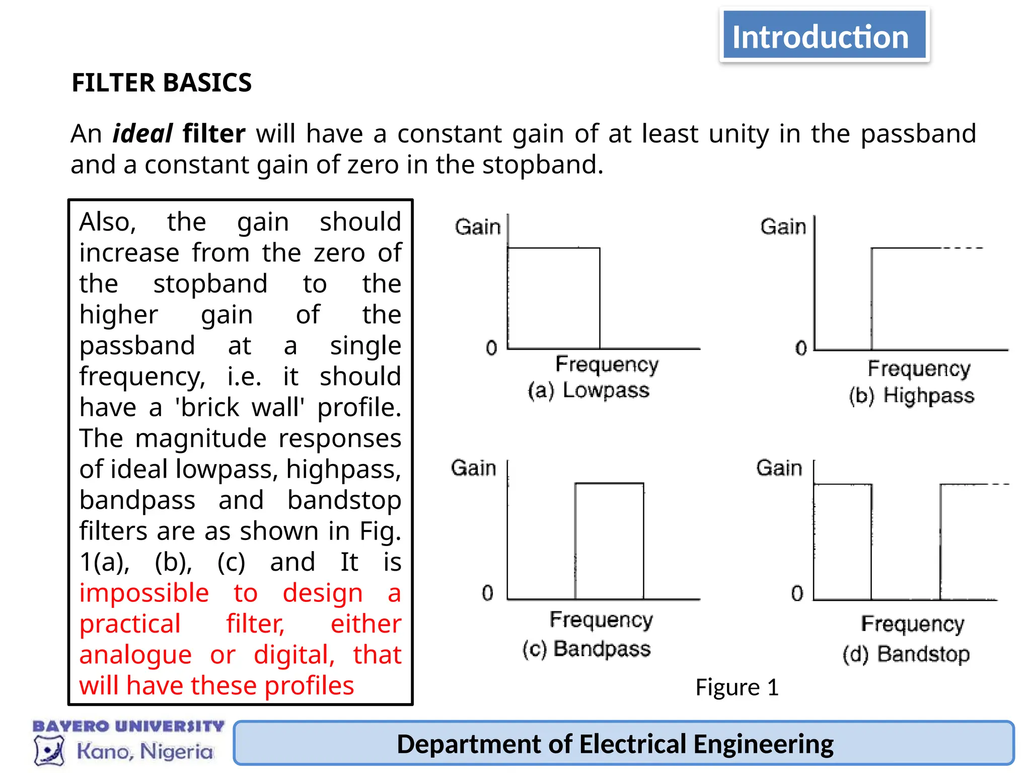
FILTER BASICS
An ideal filter will have a constant gain of at least unity in the passband
and a constant gain of zero in the stopband.
Also, the gain should
increase from the zero of
the stopband to the
higher gain of the
passband at a single
frequency, i.e. it should
have a 'brick wall' profile.
The magnitude responses
of ideal lowpass, highpass,
bandpass and bandstop
filters are as shown in Fig.
1(a), (b), (c) and It is
impossible to design a
practical filter, either
analogue or digital, that
will have these profiles Figure 1
Introduction
4.
Department of ElectricalEngineering
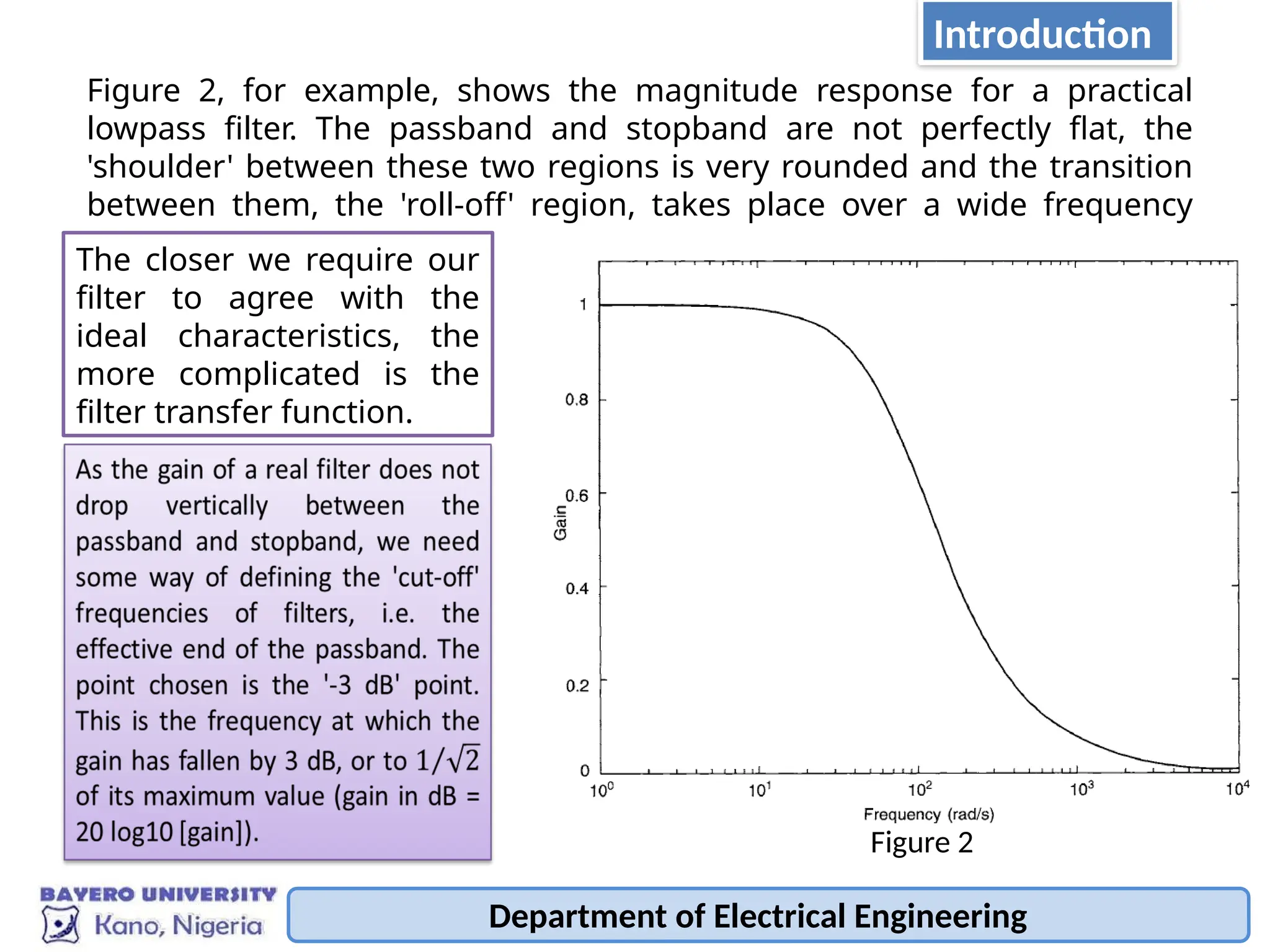
Figure 2, for example, shows the magnitude response for a practical
lowpass filter. The passband and stopband are not perfectly flat, the
'shoulder' between these two regions is very rounded and the transition
between them, the 'roll-off' region, takes place over a wide frequency
range.
The closer we require our
filter to agree with the
ideal characteristics, the
more complicated is the
filter transfer function.
Figure 2
Introduction
5.
DIRECT METHOD
Thereare several approaches that can be taken to the design of IIR
filters. One common method is to take a standard analogue filter, e.g.
Butterworth, Chebyshev, Bessell, etc., and convert this into its discrete
equivalent.
An alternative procedure is to start with the z-plane p-z diagram and
attempt to place poles and zeros so as to produce the desired frequency
response. This is often called the 'direct‘ design method.
In this method, poles and zeros are placed on the z-plane in an attempt
to achieve the required frequency response. When designing digital
filters in this way there is sometimes an element of 'trial and error'
involved.
THE DIRECT DESIGN OF IIR FILTERS
Department of Electrical Engineering
The reliance on trial and error has obviously been made much more
viable with the increased availability of CAD packages such as MATLAB.
These packages allow us to simulate and then modify our designs very
quickly.
Once a suitable p-z diagram has been established, the system transfer
function can be derived. One of the many pleasures of using digital
filters is that it is very easy to convert the transfer function into the
actual filter, i.e. to convert it into the corresponding DSP software.
6.
Digital filters arebroadly divided into two types- finite impulse response
(FIR) and infinite impulse response (IIR) filters. If a single pulse is used as
the input for an FIR filter the output pulses last for a finite time, while the
output from an IIR filter will, theoretically, continue for ever.
Generally, FIR filters are non-recursive, i.e. do not use feedback, while IIR
do.
The general expression for the transfer function, T(z), of an FIR filter is:
while that for the IIR filter is:
Although they have the disadvantage of requiring more coefficients to
achieve a similar filter performance, FIR filters do have the advantage that
they will never be unstable, unlike IIR filters. The main point is that the two
types of filter are very different in their performance and also in their design.
Department of Electrical Engineering
Introduction
7.
Department of ElectricalEngineering
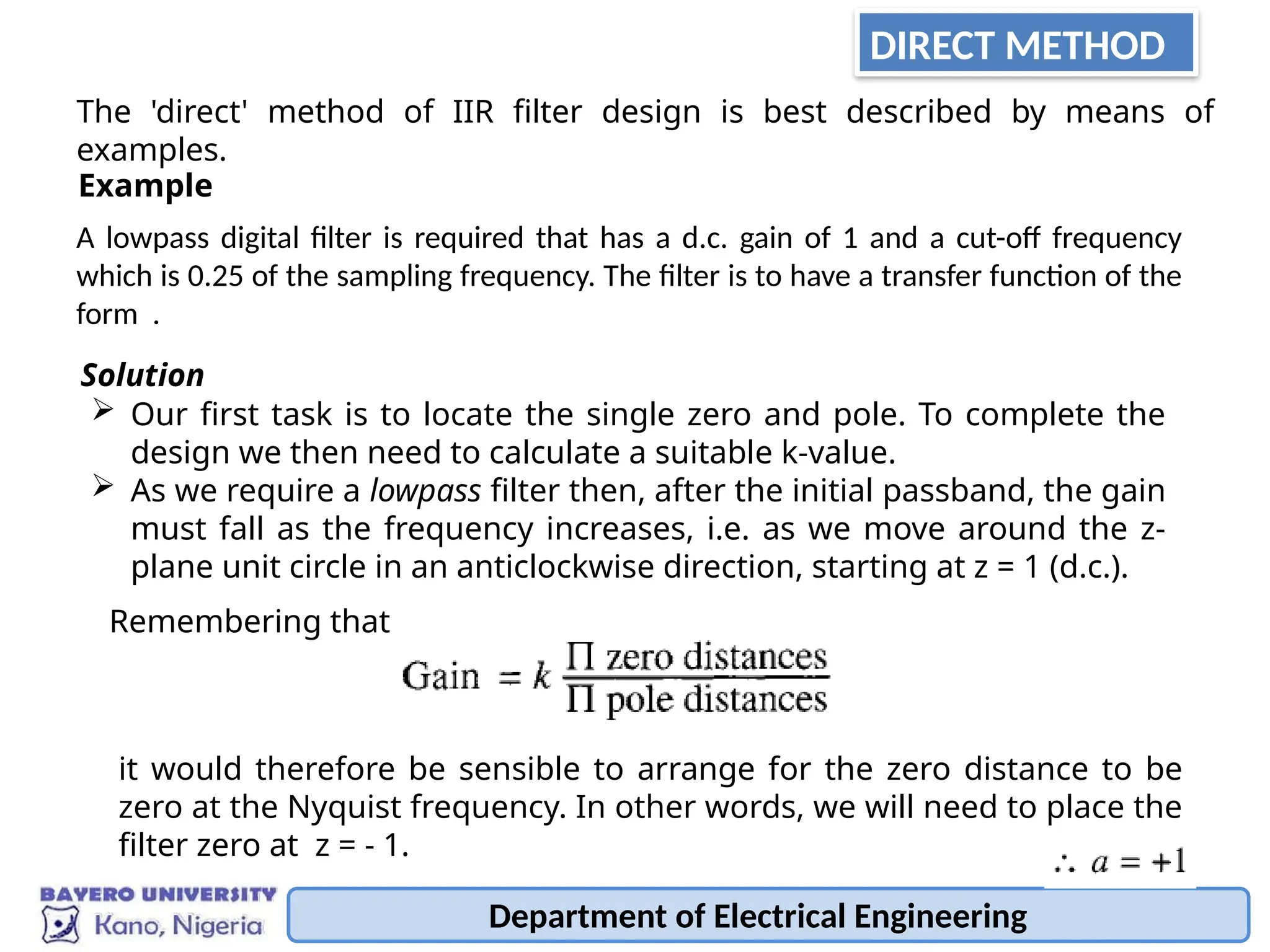
The 'direct' method of IIR filter design is best described by means of
examples.
A lowpass digital filter is required that has a d.c. gain of 1 and a cut-off frequency
which is 0.25 of the sampling frequency. The filter is to have a transfer function of the
form .
Example
Our first task is to locate the single zero and pole. To complete the
design we then need to calculate a suitable k-value.
As we require a lowpass filter then, after the initial passband, the gain
must fall as the frequency increases, i.e. as we move around the z-
plane unit circle in an anticlockwise direction, starting at z = 1 (d.c.).
Solution
it would therefore be sensible to arrange for the zero distance to be
zero at the Nyquist frequency. In other words, we will need to place the
filter zero at z = - 1.
Remembering that
DIRECT METHOD
8.
Department of ElectricalEngineering
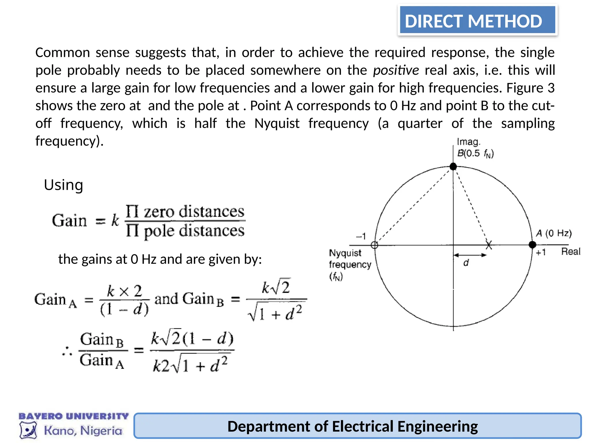
Common sense suggests that, in order to achieve the required response, the single
pole probably needs to be placed somewhere on the positive real axis, i.e. this will
ensure a large gain for low frequencies and a lower gain for high frequencies. Figure 3
shows the zero at and the pole at . Point A corresponds to 0 Hz and point B to the cut-
off frequency, which is half the Nyquist frequency (a quarter of the sampling
frequency).
Using
the gains at 0 Hz and are given by:
DIRECT METHOD
9.
Department of ElectricalEngineering
But B is the -3 dB point, therefore
Therefore the pole must be placed at the
origin.
DIRECT METHOD
10.
Department of ElectricalEngineering
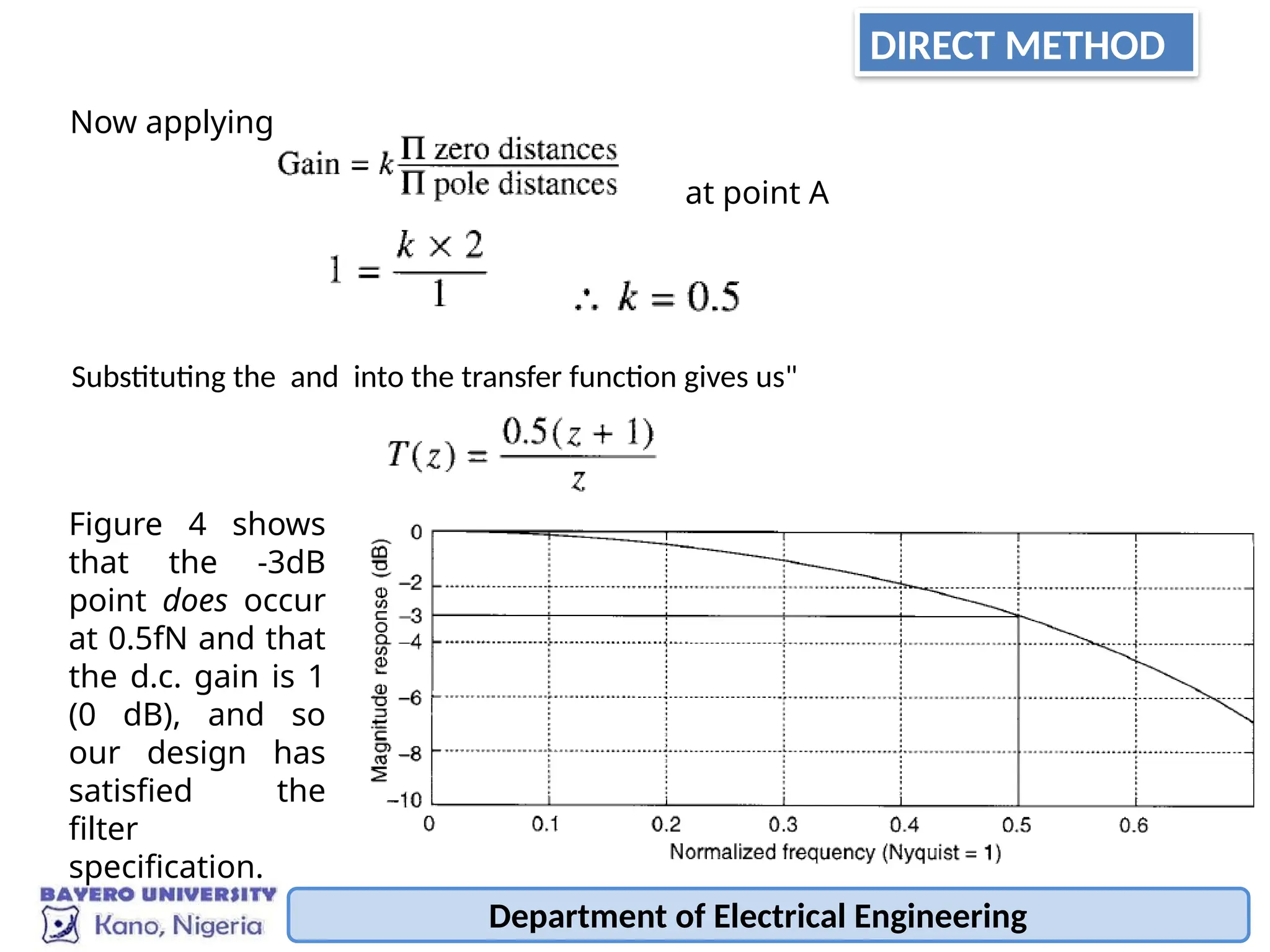
Now applying
at point A
Substituting the and into the transfer function gives us"
Figure 4 shows
that the -3dB
point does occur
at 0.5fN and that
the d.c. gain is 1
(0 dB), and so
our design has
satisfied the
filter
specification.
DIRECT METHOD
11.
Department of ElectricalEngineering
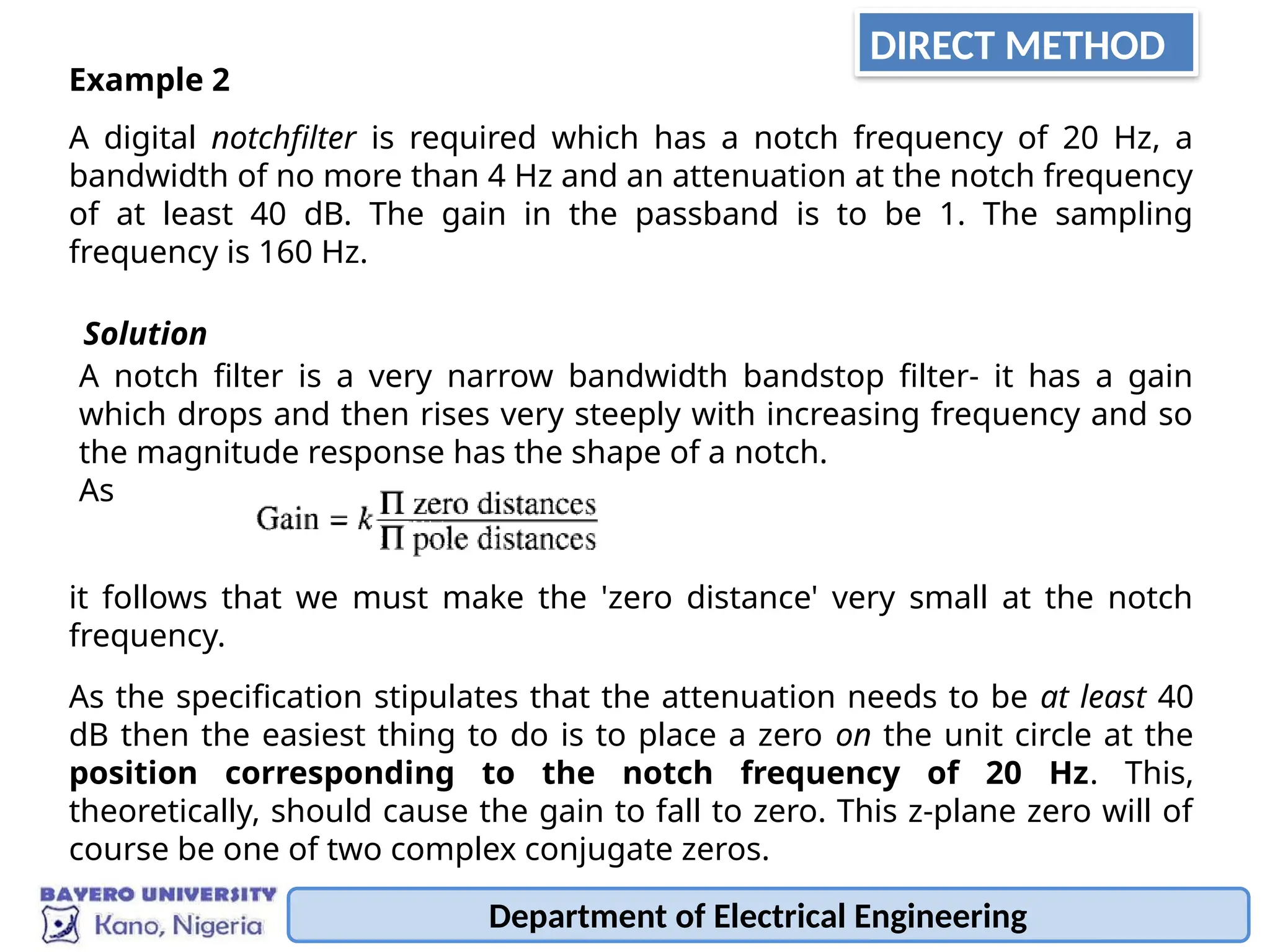
Example 2
A digital notchfilter is required which has a notch frequency of 20 Hz, a
bandwidth of no more than 4 Hz and an attenuation at the notch frequency
of at least 40 dB. The gain in the passband is to be 1. The sampling
frequency is 160 Hz.
Solution
A notch filter is a very narrow bandwidth bandstop filter- it has a gain
which drops and then rises very steeply with increasing frequency and so
the magnitude response has the shape of a notch.
As
it follows that we must make the 'zero distance' very small at the notch
frequency.
As the specification stipulates that the attenuation needs to be at least 40
dB then the easiest thing to do is to place a zero on the unit circle at the
position corresponding to the notch frequency of 20 Hz. This,
theoretically, should cause the gain to fall to zero. This z-plane zero will of
course be one of two complex conjugate zeros.
DIRECT METHOD
12.
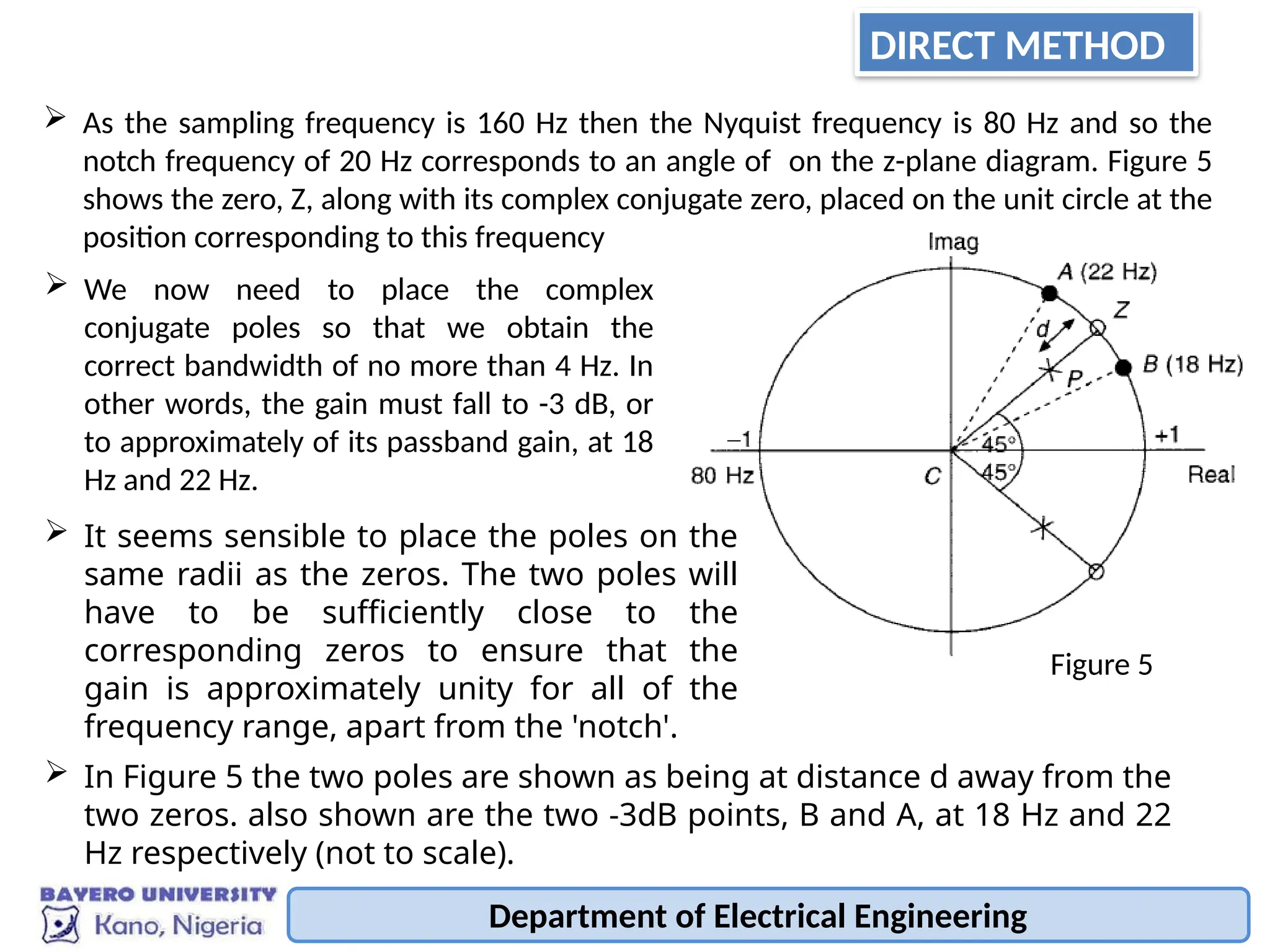
Department of ElectricalEngineering
As the sampling frequency is 160 Hz then the Nyquist frequency is 80 Hz and so the
notch frequency of 20 Hz corresponds to an angle of on the z-plane diagram. Figure 5
shows the zero, Z, along with its complex conjugate zero, placed on the unit circle at the
position corresponding to this frequency
We now need to place the complex
conjugate poles so that we obtain the
correct bandwidth of no more than 4 Hz. In
other words, the gain must fall to -3 dB, or
to approximately of its passband gain, at 18
Hz and 22 Hz.
It seems sensible to place the poles on the
same radii as the zeros. The two poles will
have to be sufficiently close to the
corresponding zeros to ensure that the
gain is approximately unity for all of the
frequency range, apart from the 'notch'.
In Figure 5 the two poles are shown as being at distance d away from the
two zeros. also shown are the two -3dB points, B and A, at 18 Hz and 22
Hz respectively (not to scale).
Figure 5
DIRECT METHOD
13.
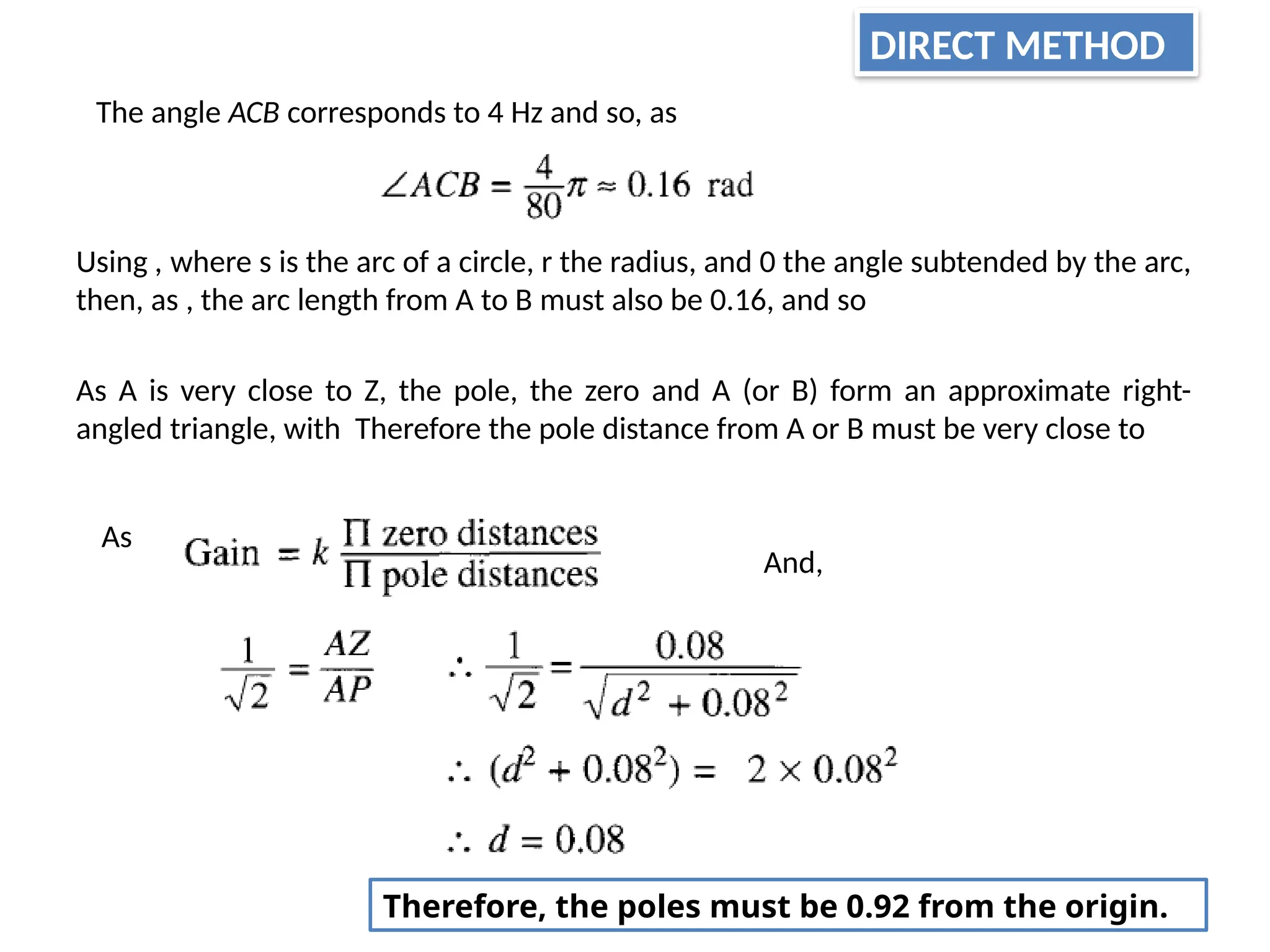
The angle ACBcorresponds to 4 Hz and so, as
Using , where s is the arc of a circle, r the radius, and 0 the angle subtended by the arc,
then, as , the arc length from A to B must also be 0.16, and so
As A is very close to Z, the pole, the zero and A (or B) form an approximate right-
angled triangle, with Therefore the pole distance from A or B must be very close to
As
And,
Therefore, the poles must be 0.92 from the origin.
DIRECT METHOD
14.
Department of ElectricalEngineering
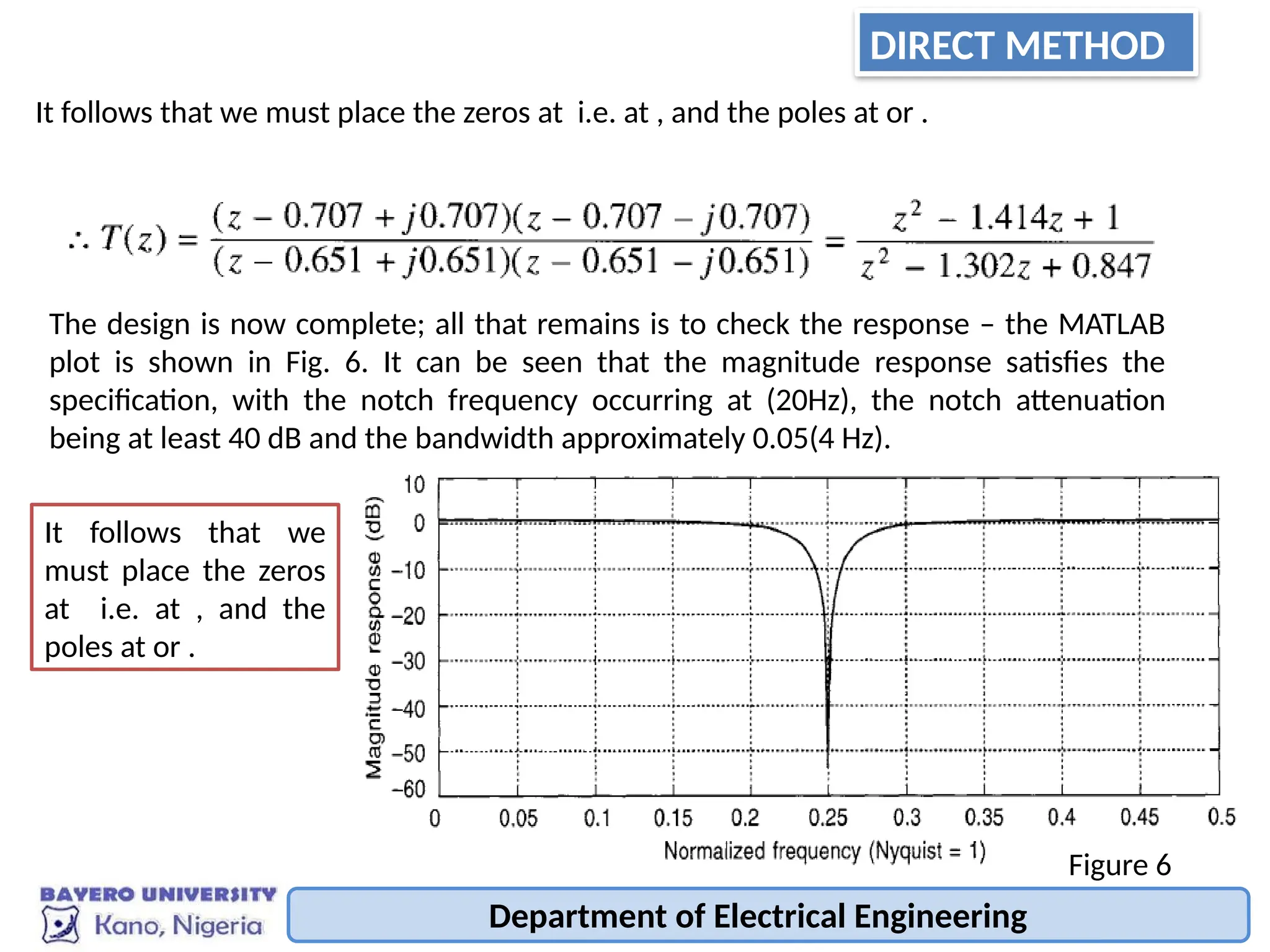
It follows that we must place the zeros at i.e. at , and the poles at or .
The design is now complete; all that remains is to check the response – the MATLAB
plot is shown in Fig. 6. It can be seen that the magnitude response satisfies the
specification, with the notch frequency occurring at (20Hz), the notch attenuation
being at least 40 dB and the bandwidth approximately 0.05(4 Hz).
Figure 6
It follows that we
must place the zeros
at i.e. at , and the
poles at or .
DIRECT METHOD
15.
Department of ElectricalEngineering
The direct design method can give reasonable results for fairly simple
filters. However, it is far from ideal when something rather more
sophisticated is needed, and so an alternative approach is required.
DESIGN OF IIR FILTERS VIA ANALOGUE FILTERS
One alternative is to used analogue filters when designing digital
filters. Various s-domain to z-domain transforms have been developed
which allow us to convert analogue filters into their digital 'equivalents'
fairly easily.
Remembered that all transforms are approximations and that no
digital filter can be identical to its analogue prototype, i.e. have
exactly the same magnitude, phase and time responses. The various s-
to-z transformation methods have advantages and disadvantages.
There are many standard methods of converting an analogue filter to
its digital equivalent- a process called 'discretization'. We will look at
three of the most common - the bilinear transform, the impulse-
invariant method and the pole-zero matching technique.
16.
Department of ElectricalEngineering
BILINEAR METHOD
There are classic analogue filters (such as; Butterworth, Chebyshev, 'elliptic'
etc.) which we can use as templates when we need to design a digital filter.
To demonstrate the various conversion steps, a simple first-order, lowpass
filter having the transfer function will be used:
THE BILINEAR TRANSFORM
This transfer function defines a lowpassfilter with a cut-off angular frequency of . For
example, if we choose , then:
or
17.
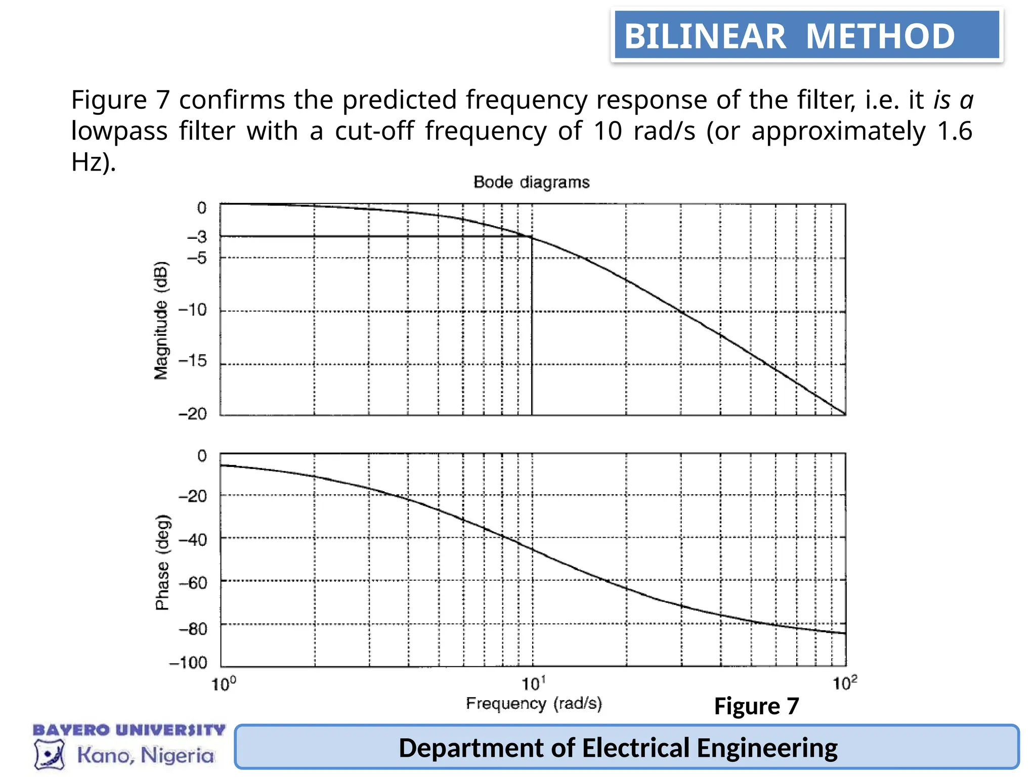
Figure 7 confirmsthe predicted frequency response of the filter, i.e. it is a
lowpass filter with a cut-off frequency of 10 rad/s (or approximately 1.6
Hz).
Department of Electrical Engineering
Figure 7
BILINEAR METHOD
18.
To apply thebilinear transform we have to replace with:
whereis the sampling period.
We will now convert the analogue lowpass
filter to its discrete equivalent using a sampling
frequency of ().
Department of Electrical Engineering
BILINEAR METHOD
19.
Department of ElectricalEngineering
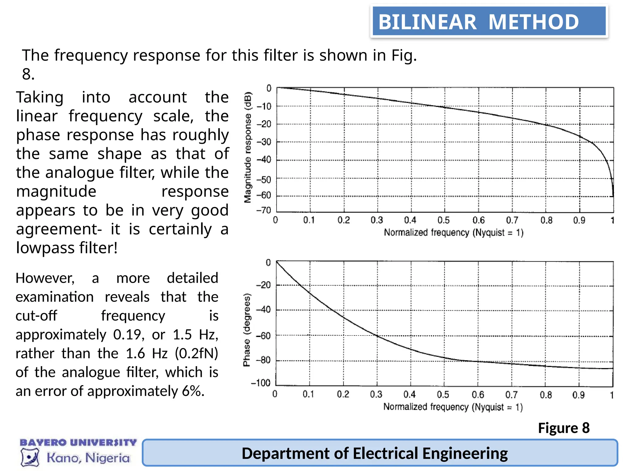
The frequency response for this filter is shown in Fig.
8.
Figure 8
Taking into account the
linear frequency scale, the
phase response has roughly
the same shape as that of
the analogue filter, while the
magnitude response
appears to be in very good
agreement- it is certainly a
lowpass filter!
However, a more detailed
examination reveals that the
cut-off frequency is
approximately 0.19, or 1.5 Hz,
rather than the 1.6 Hz (0.2fN)
of the analogue filter, which is
an error of approximately 6%.
BILINEAR METHOD
20.
Department of ElectricalEngineering
If the approximation is too poor to be acceptable, then we need to
'pre-warp' the frequencies before we apply the bilinear
transformation.
'
c
In this example we have
just one frequency which
is of obvious interest – the
single breakpoint of 10
rad/s.
We now need to redesign the digital filter starting with the 'pre-warped' s domain
transfer function. There are several ways of doing this, but the easiest is to first
change the format of the transfer function such that every s is replaced with .
So, dividing numerator and denominator by 10,
our simple transfer function now becomes:
BILINEAR METHOD
21.
Department of ElectricalEngineering
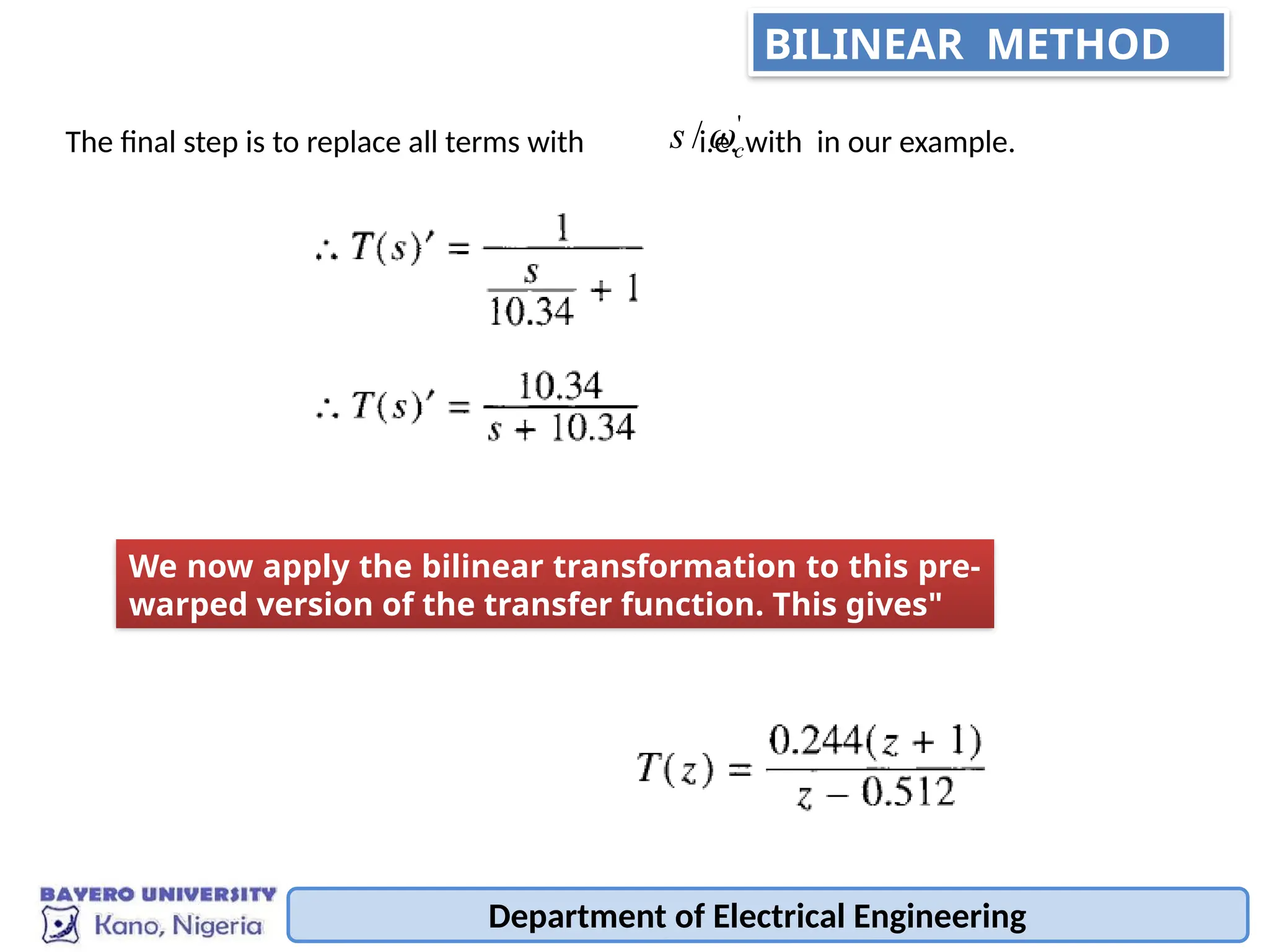
The final step is to replace all terms with i.e. with in our example.
'
/ c
s
We now apply the bilinear transformation to this pre-
warped version of the transfer function. This gives"
BILINEAR METHOD
22.
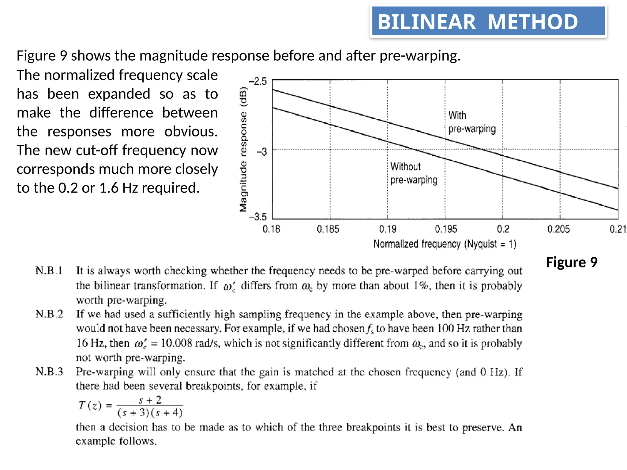
Figure 9 showsthe magnitude response before and after pre-warping.
Figure 9
The normalized frequency scale
has been expanded so as to
make the difference between
the responses more obvious.
The new cut-off frequency now
corresponds much more closely
to the 0.2 or 1.6 Hz required.
BILINEAR METHOD
23.
A continuous filterhas a transfer function of
It is to be converted to its digital equivalent using the bilinear transform. It
is important that the gain is preserved at the upper breakpoint frequency
of 2 rad/s. The sampling frequency used is 2 Hz.
Example 3
We first need to check whether pre-warping is necessary to maintain the
breakpoints.
Using
Solution
As the difference between and is significant (about 10%), then pre-warping
is necessary.
'
c
Department of Electrical Engineering
BILINEAR METHOD
24.
Department of ElectricalEngineering
Changing the format of the transfer function by replacing all s-values with , i.e. , gives:
(Here we have divided both bracketed terms by 2, in other words we have
divided the denominator by 4. We therefore also need to divide the
numerator by 4-hence the '0.5'.)
Replacing all terms with :
Applying the bilinear transform, i.e. replacing with results in the z-domain transfer
function of:
BILINEAR METHOD
25.
Department of ElectricalEngineering
IMPULSE-METHOD
THE IMPULSE-INVARIANT METHOD
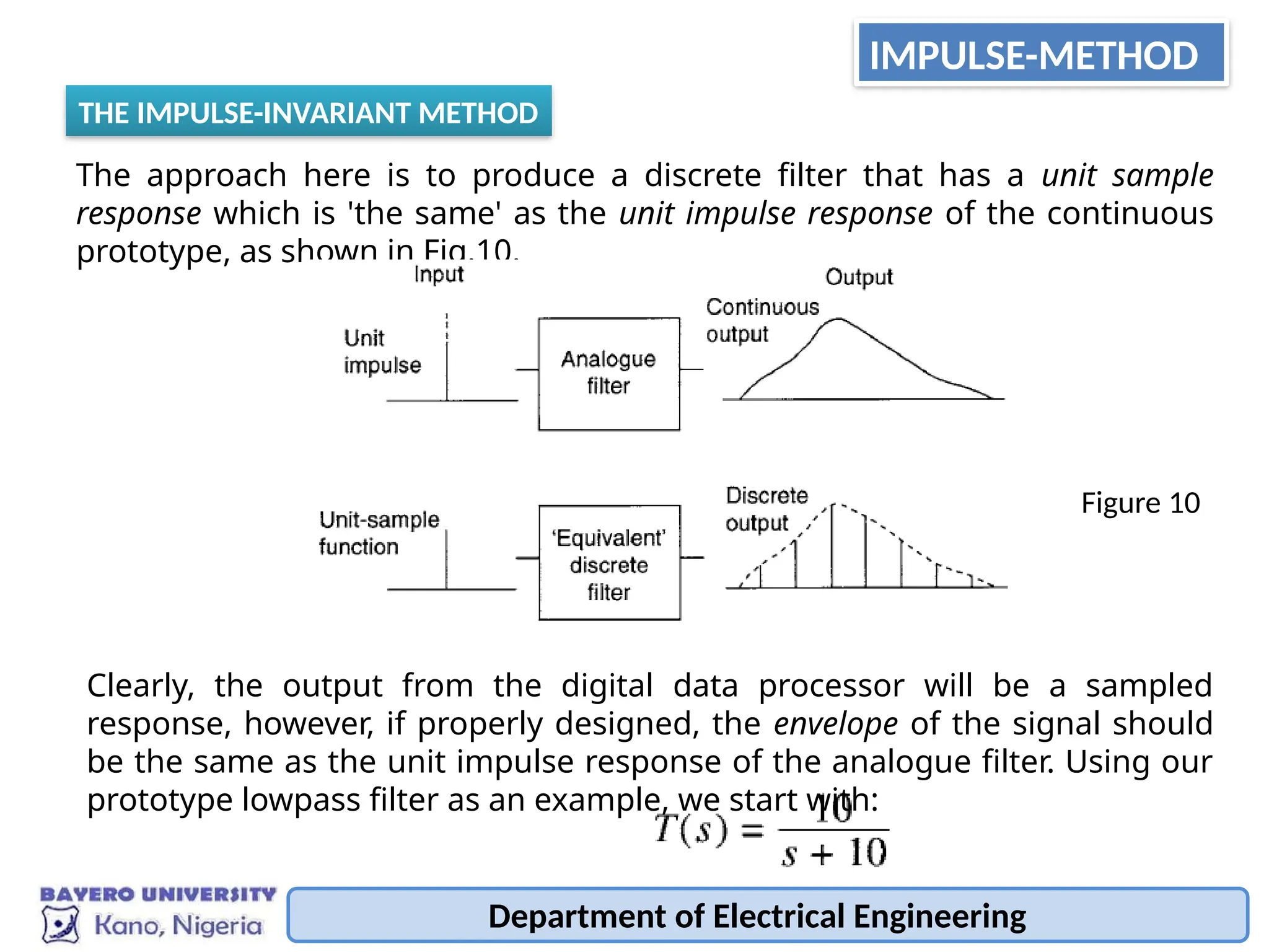
The approach here is to produce a discrete filter that has a unit sample
response which is 'the same' as the unit impulse response of the continuous
prototype, as shown in Fig.10.
Figure 10
Clearly, the output from the digital data processor will be a sampled
response, however, if properly designed, the envelope of the signal should
be the same as the unit impulse response of the analogue filter. Using our
prototype lowpass filter as an example, we start with:
26.
Department of ElectricalEngineering
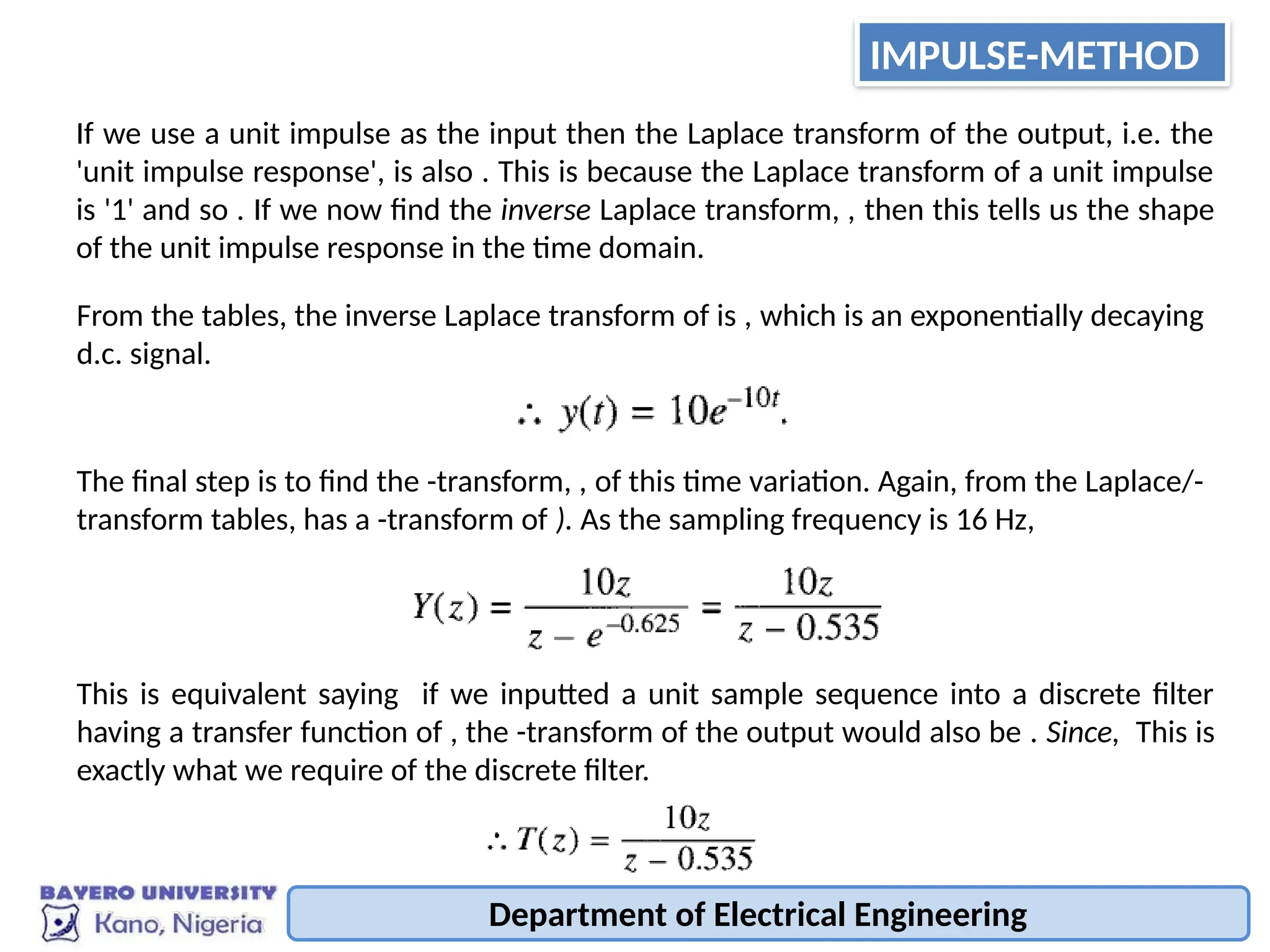
If we use a unit impulse as the input then the Laplace transform of the output, i.e. the
'unit impulse response', is also . This is because the Laplace transform of a unit impulse
is '1' and so . If we now find the inverse Laplace transform, , then this tells us the shape
of the unit impulse response in the time domain.
From the tables, the inverse Laplace transform of is , which is an exponentially decaying
d.c. signal.
The final step is to find the -transform, , of this time variation. Again, from the Laplace/-
transform tables, has a -transform of ). As the sampling frequency is 16 Hz,
This is equivalent saying if we inputted a unit sample sequence into a discrete filter
having a transfer function of , the -transform of the output would also be . Since, This is
exactly what we require of the discrete filter.
IMPULSE-METHOD
27.
Department of ElectricalEngineering
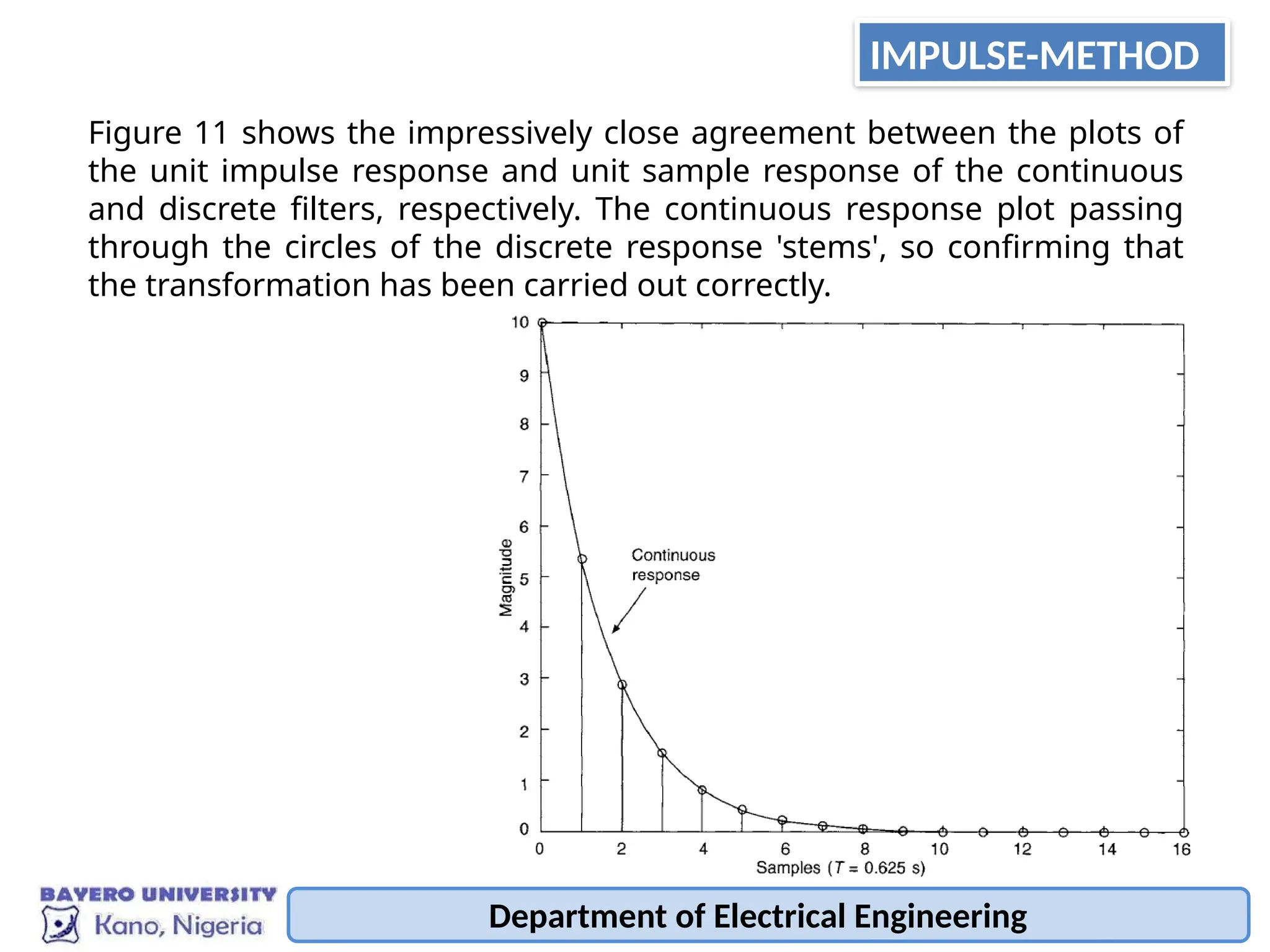
Figure 11 shows the impressively close agreement between the plots of
the unit impulse response and unit sample response of the continuous
and discrete filters, respectively. The continuous response plot passing
through the circles of the discrete response 'stems', so confirming that
the transformation has been carried out correctly.
IMPULSE-METHOD
28.
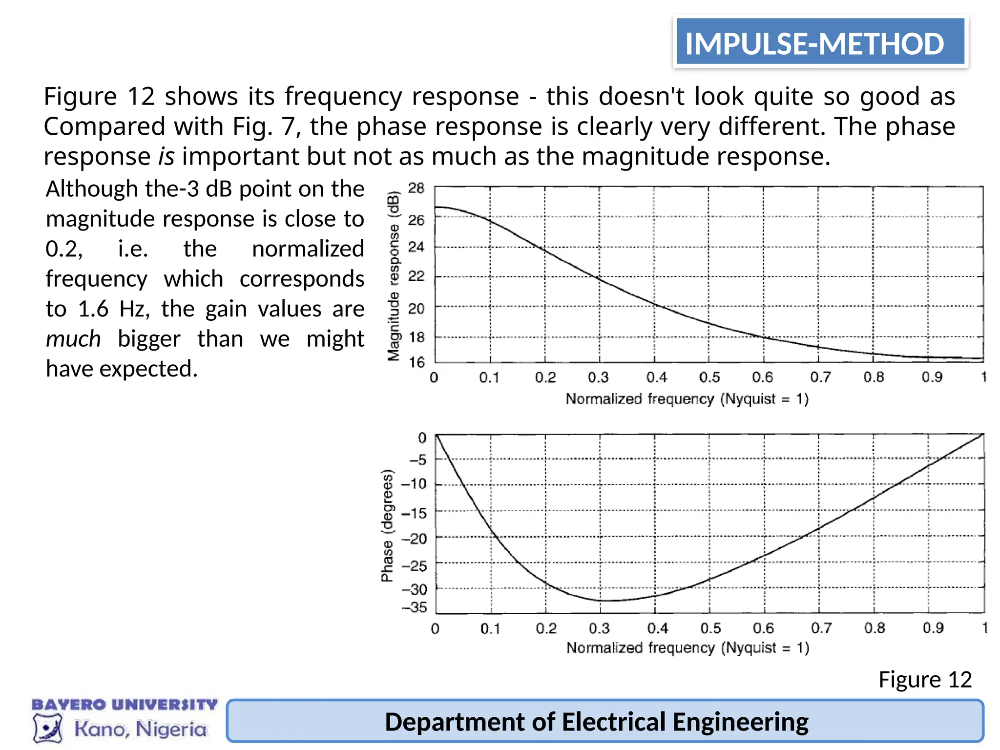
Figure 12 showsits frequency response - this doesn't look quite so good as
Compared with Fig. 7, the phase response is clearly very different. The phase
response is important but not as much as the magnitude response.
Although the-3 dB point on the
magnitude response is close to
0.2, i.e. the normalized
frequency which corresponds
to 1.6 Hz, the gain values are
much bigger than we might
have expected.
Department of Electrical Engineering
Figure 12
IMPULSE-METHOD
29.
Department of ElectricalEngineering
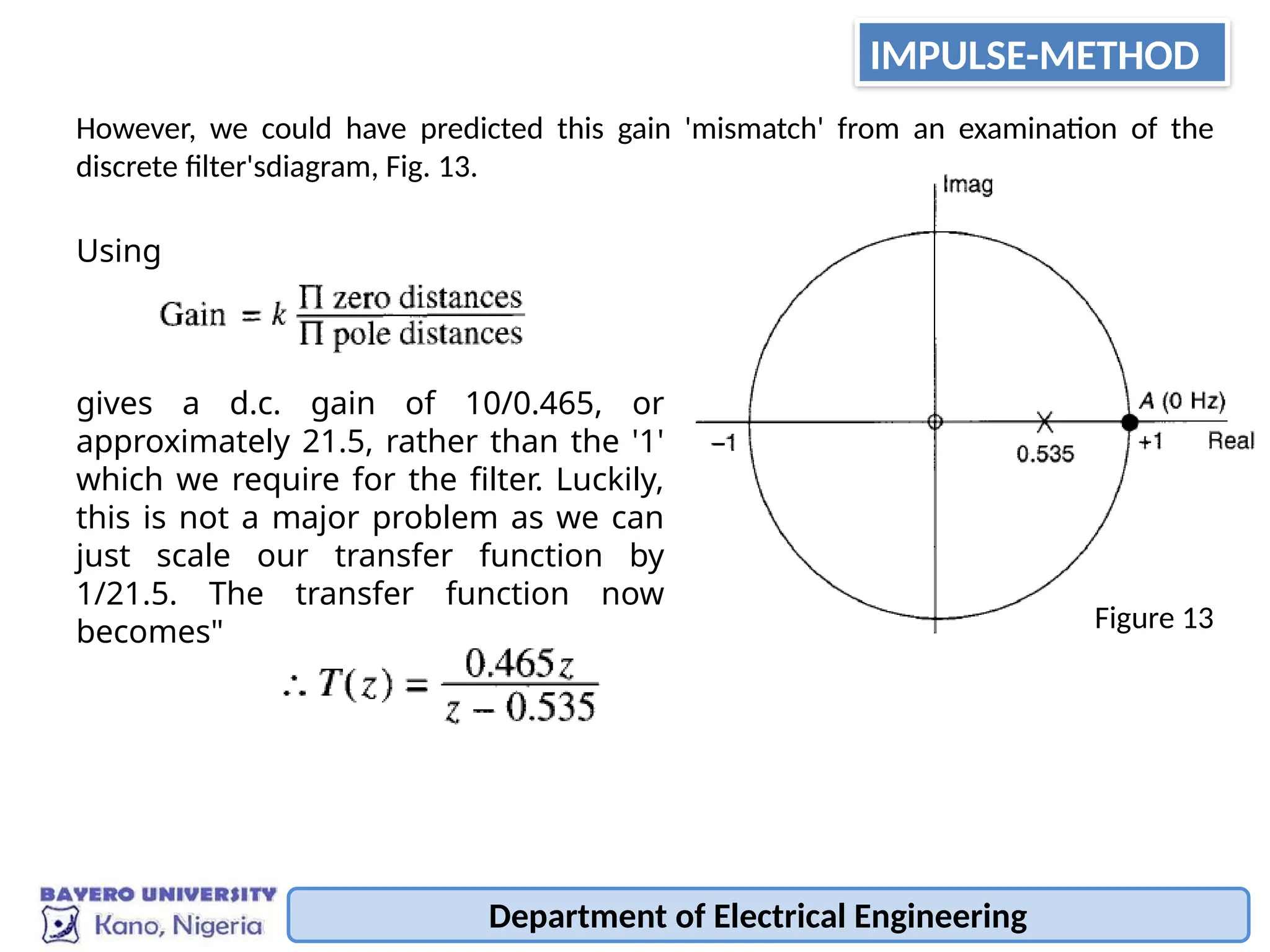
However, we could have predicted this gain 'mismatch' from an examination of the
discrete filter'sdiagram, Fig. 13.
Using
gives a d.c. gain of 10/0.465, or
approximately 21.5, rather than the '1'
which we require for the filter. Luckily,
this is not a major problem as we can
just scale our transfer function by
1/21.5. The transfer function now
becomes" Figure 13
IMPULSE-METHOD
30.
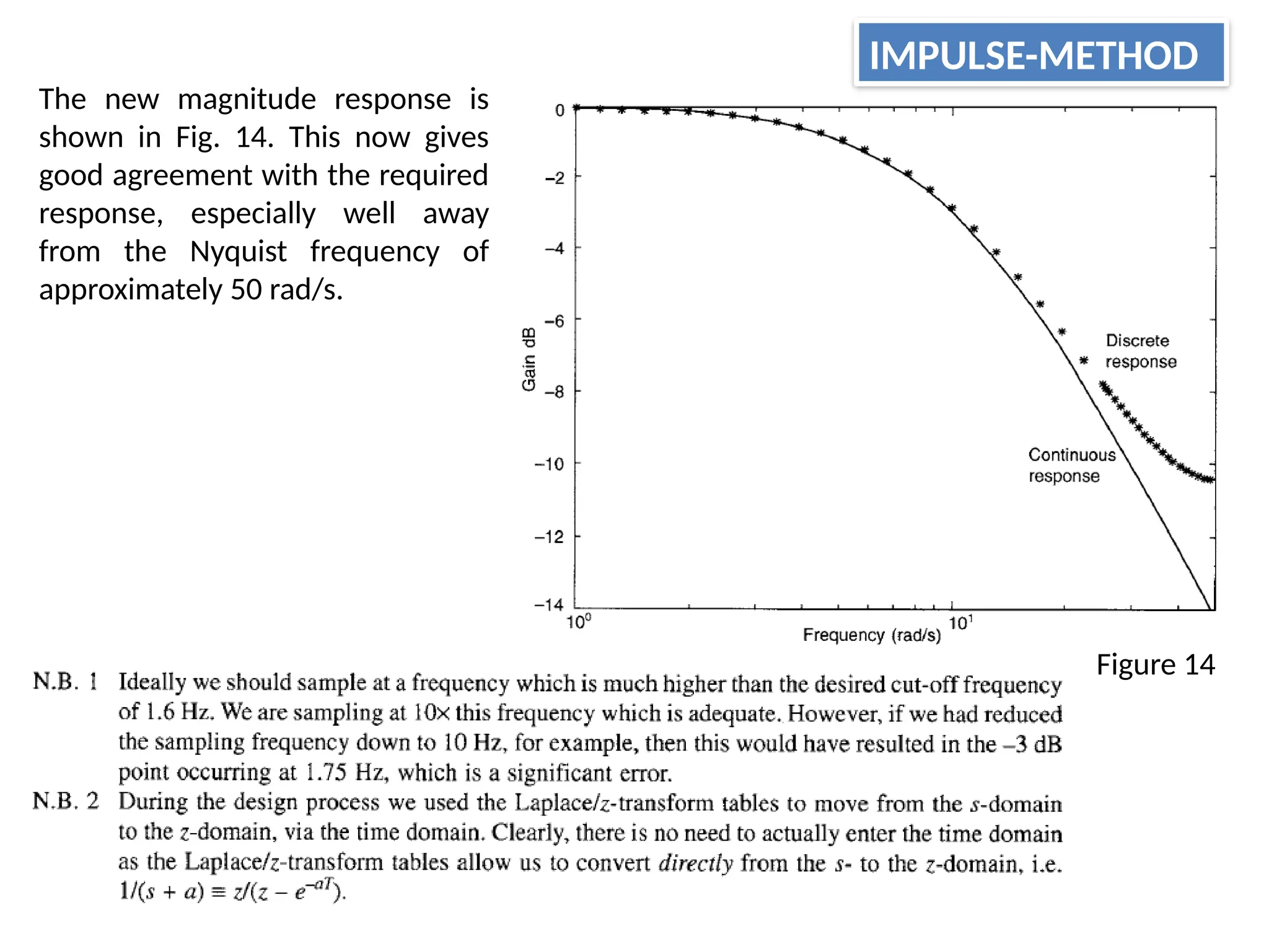
The new magnituderesponse is
shown in Fig. 14. This now gives
good agreement with the required
response, especially well away
from the Nyquist frequency of
approximately 50 rad/s.
Figure 14
IMPULSE-METHOD
31.
Department of ElectricalEngineering
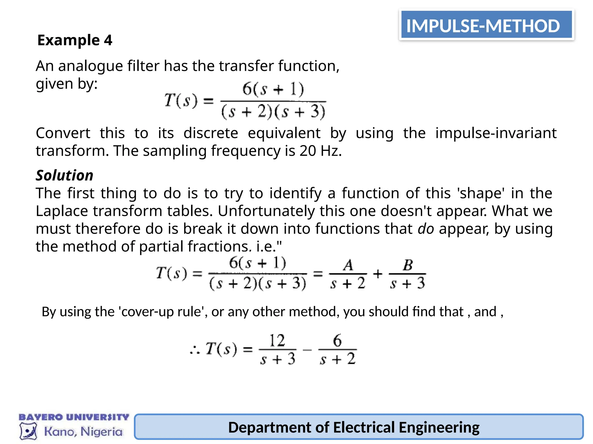
An analogue filter has the transfer function,
given by:
Example 4
Convert this to its discrete equivalent by using the impulse-invariant
transform. The sampling frequency is 20 Hz.
Solution
The first thing to do is to try to identify a function of this 'shape' in the
Laplace transform tables. Unfortunately this one doesn't appear. What we
must therefore do is break it down into functions that do appear, by using
the method of partial fractions, i.e."
By using the 'cover-up rule', or any other method, you should find that , and ,
IMPULSE-METHOD
32.
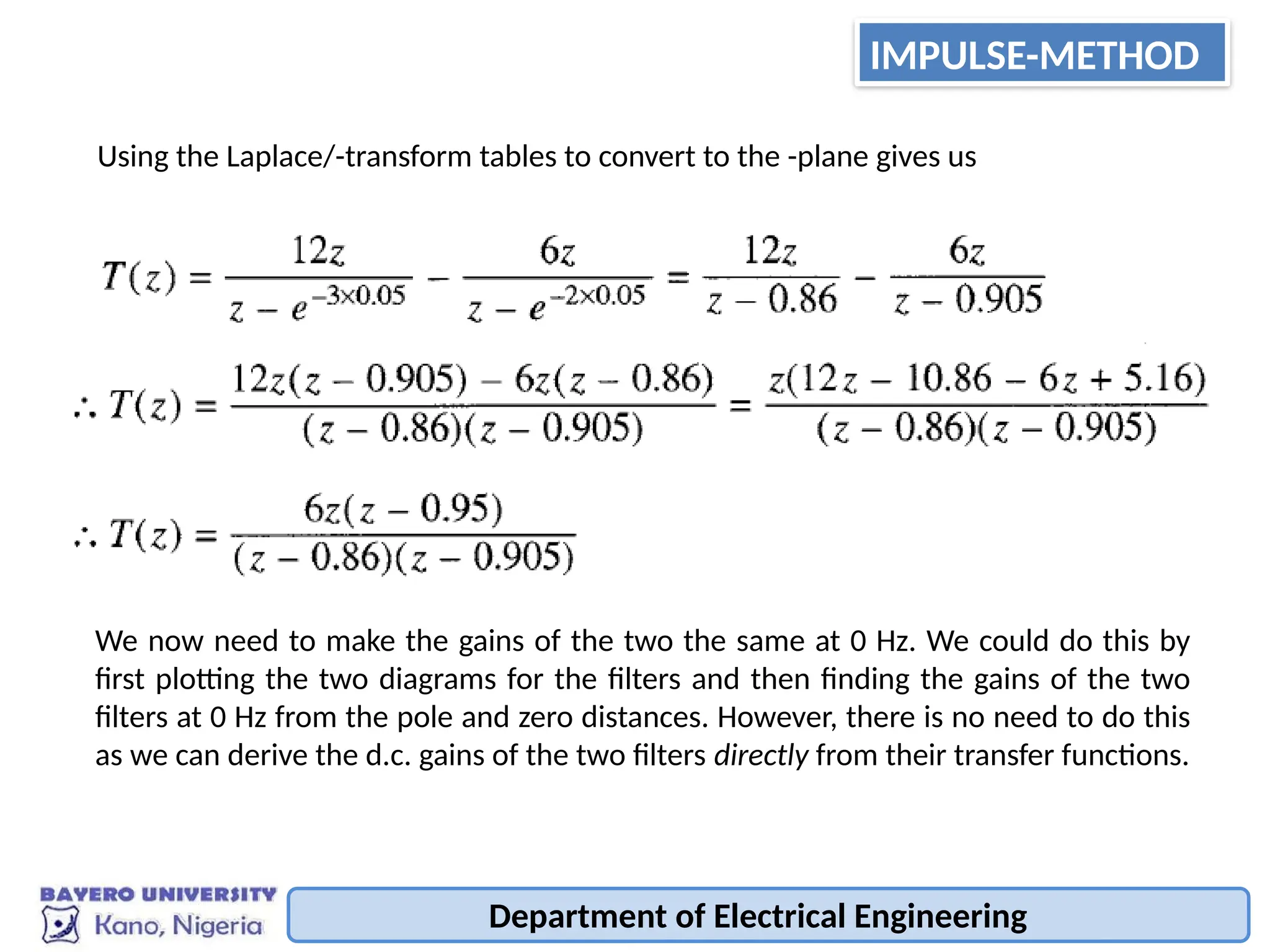
Using the Laplace/-transformtables to convert to the -plane gives us
We now need to make the gains of the two the same at 0 Hz. We could do this by
first plotting the two diagrams for the filters and then finding the gains of the two
filters at 0 Hz from the pole and zero distances. However, there is no need to do this
as we can derive the d.c. gains of the two filters directly from their transfer functions.
Department of Electrical Engineering
IMPULSE-METHOD
33.
Department of ElectricalEngineering
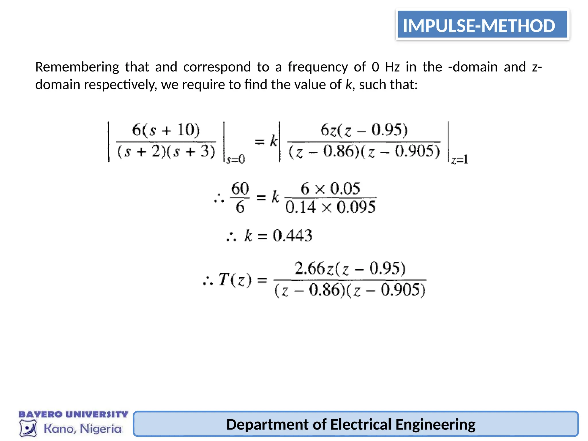
Remembering that and correspond to a frequency of 0 Hz in the -domain and z-
domain respectively, we require to find the value of k, such that:
IMPULSE-METHOD
34.
Department of ElectricalEngineering
POLE-ZERO MAPPING
POLE-ZERO MAPPING
The approach adopted here is to use the relationship z- e sTto convert the -plane
poles and zeros of the continuous filter to equivalent poles and zeros in the -plane.
Once the -plane poles and zeros are known, the general form of the -domain transfer
function can be derived.
All that then remains to be done is to ensure that the two filters have the same gain,
at least at some important frequency -often 0 Hz.
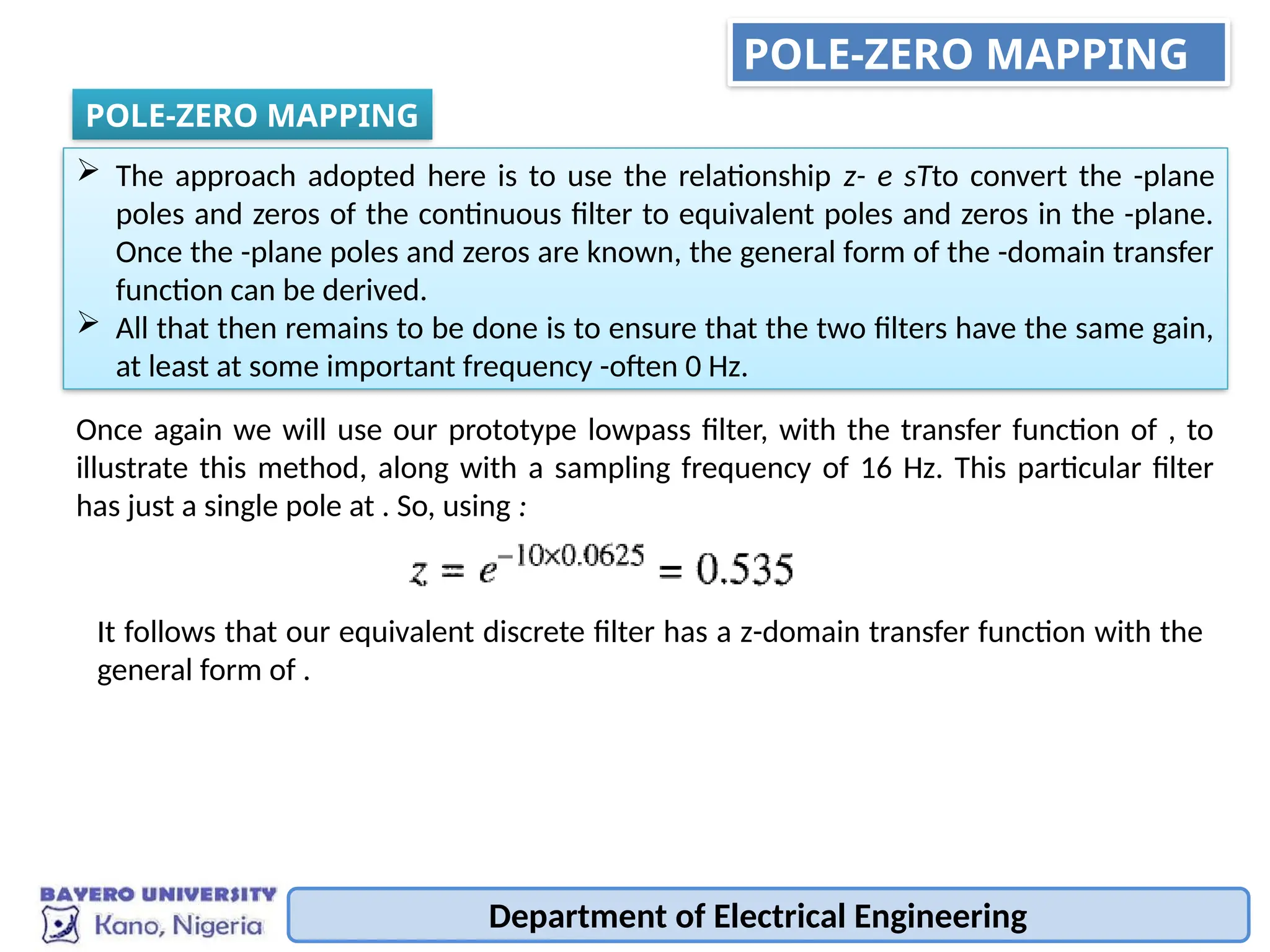
Once again we will use our prototype lowpass filter, with the transfer function of , to
illustrate this method, along with a sampling frequency of 16 Hz. This particular filter
has just a single pole at . So, using :
It follows that our equivalent discrete filter has a z-domain transfer function with the
general form of .
35.
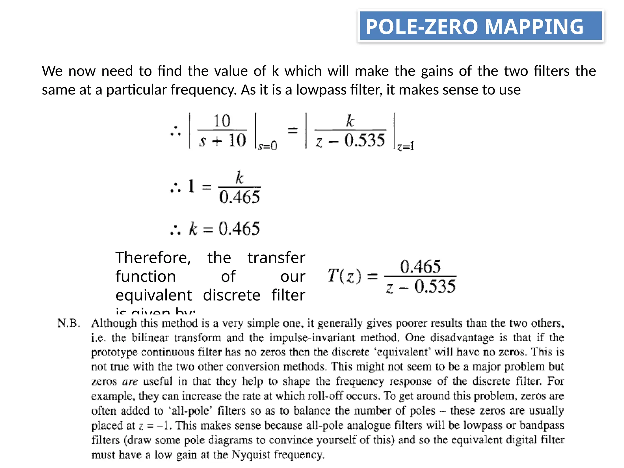
We now needto find the value of k which will make the gains of the two filters the
same at a particular frequency. As it is a lowpass filter, it makes sense to use
Therefore, the transfer
function of our
equivalent discrete filter
is given by:
POLE-ZERO MAPPING
36.
Department of ElectricalEngineering
For the d.c. gains of the continuous and discrete filters to be the same, we require that
.
Our filter design should therefore be improved if we add a single zero at . The transfer
function now becomes:
POLE-ZERO MAPPING