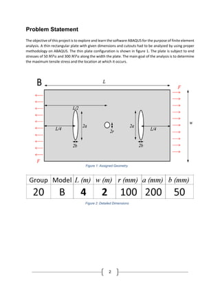
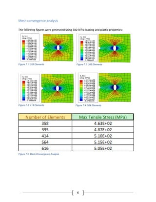
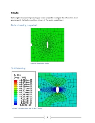
1
Mechanics of Deformable Solids
MECH 321
Final Project
April 16th, 2018
Chris Jing 260634735
Stasik Nemirovsky 260660024
2
Problem Statement
The objective of this project is to explore and learn the software ABAQUS for the purpose of finite element
analysis. A thin rectangular plate with given dimensions and cutouts had to be analyzed by using proper
methodology on ABAQUS. The thin plate configuration is shown in figure 1. The plate is subject to end
stresses of 50 𝑀𝑃𝑎 and 300 𝑀𝑃𝑎 along the width the plate. The main goal of the analysis is to determine
the maximum tensile stress and the location at which it occurs.
Figure 1: Assigned Geometry
Figure 2: Detailed Dimensions
3
Setup of FE Model
Drawn Geometry:
Figure 3: Drawn Geometry
Figure 3 displays the geometry assigned to our group, drawn in ABAQUS. From simple inspection,
it is obvious that the plate can be considered symmetric about the red dotted line in the figure
above. Drawing the geometry of the plate is the first step in the analysis process. Proper
dimensions and geometry are crucial for successful and accurate results.
Boundary and Loading Conditions
Due to an axis of symmetry, in the middle of the plate, it is enough to create just half of the geometry
in ABAQUS. The right half of the geometry was used for the rest of the process. Due to symmetry, the
left half of the plate will have the same stress distribution as the right half. Analyzing the reduced
geometry greatly reduces the number of elements needed to solve for the maximum tensile stress in
the plate. The reduced geometry is as shown below:
4
Following the reduced geometry, boundary and loading condition are as shown below:
Figure 5 displays the boundary and loading conditions that were applied to our geometry. The
purple arrows on the right hand side represent a uniform load of 50 or 300 𝑀𝑃𝑎, depending on
the case analyzed. In addition, the appropriate boundary conditions are used to fix the left edge,
in both X and Y directions.
Material Properties
In all the considered cases, the plate is made of steel with the following properties:
 𝐸 = 200 𝐺𝑃𝑎 (Young’s modulus)
 𝜐 = 0.3 (Poisson’s ratio)
Figure 4: Reduced Geometry Due To Symmetry
Figure 5: Boundary and Loading Conditions
F
F
F
5
In Addition, for part D only the following plastic properties were added:
From the provided Stress Vs. Strain diagram (Figure 6), it is found that the yield stress of our plate
is approximately 400 𝑀𝑃𝑎 and has 10% strain deformation at 800 𝑀𝑃𝑎.
Element type
The next step in the setup process was choosing the element type. Our assigned geometry features 2D
thin rectangular plate. Therefore, plain stress element type was chosen. Plain stress element type assumes
there are no stresses in the “Z” direction, since the analyzed part is thin enough to neglect those. This
allows to simply explore the strains and stresses in the X and Y directions.
Number of Elements
The number of elements used in the analysis has a crucial impact on the quality of the results. In general,
more elements means approximations that are more accurate but also much higher computational
complexity, which results in longer processing times. Therefore, in order to analyze the geometry
accurately and efficiently, experimentation with increasing amounts of elements is required until the
value of max tensile stress starts to converge to a certain value (mesh convergence). In this project, the
max amount of elements was limited to 1000. However, it was found that the max tensile stress begins to
plateau, above roughly 414 elements.
Figure 6: Stress Vs. Strain for Plastic Properties
6
Mesh convergence analysis
The following figures were generated using 300 𝑀𝑃𝑎 loading and plastic properties:
Figure 7.1: 358 Elements Figure 7.2: 395 Elements
Figure 7.3: 414 Elements Figure 7.4: 564 Elements
Figure 7.5: Mesh Convergence Analysis
7
`
Following the information displayed in figure 7.6, it was decided to perform the next steps in the
analysis process using a mesh with exactly 414 elements, which corresponds to the mesh convergence
analysis.
Figure 7.6: Mesh convergence - Number of Elements Vs. Max Tensile Stress
8
Results
Following the mesh convergence analysis, we can proceed to investigate the deformation of our
geometry with the loading conditions of interest. The results are as follows:
Before Loading is applied:
50 MPa Loading:
Figure 9: Deformed Shape with 50 MPa Loading
Figure 8: Undeformed Shape
9
The Max tensile stress for the 50 MPa Loading condition, was found to be 160.8 𝑀𝑃𝑎. From figure 9, it is
obvious that the Max Stress occurs at the top and bottom of the slot in the middle of the figure.
300 MPa Loading:
For the 300 𝑀𝑃𝑎 loading case the max tensile stress was found to be 883.6 𝑀𝑃𝑎. Similarly, to the previous
case the Max Stress occurs at the top and bottom of the slot in the middle of the figure.
Stress Concentration Factor
Following the results shown above, we are able to find the stress concentration factor of the slots in our
plate. To find the exact values, the following formula is used:
𝑲 𝒕 =
𝝈 𝒎𝒂𝒙
𝝈 𝒏𝒐𝒎𝒊𝒏𝒂𝒍
(1)
𝑲 𝒕 =
𝟏𝟔𝟎.𝟖 𝑴𝑷𝒂
𝟓𝟎 𝑴𝑷𝒂
= 𝟑. 𝟐𝟐 (2)
Figure 10: Deformed Shape with 300 MPa Loading
10
Simulation with Plastic Properties
In the next step, plastic properties from figure 6 are introduced into the simulation. Using the same
boundary and loading conditions, we reach the following results:
50 MPa Loading:
For the 50 𝑀𝑃𝑎 loading we see no difference in the max stresses in the part. The reason being is the fact
that even with the stress concentrations, the stresses never exceed the yield stress (400 𝑀𝑃𝑎) and
therefore the plate still behave in an elastic manner at all times.
𝑲 𝒕 =
𝟏𝟔𝟎.𝟖 𝑴𝑷𝒂
𝟓𝟎 𝑴𝑷𝒂
= 𝟑. 𝟐𝟐 (3)
Figure 11: Deformed Shape with 50 MPa Loading and Plastic Properties
11
300 MPa Loading:
For the 300 𝑀𝑃𝑎 loading we see a significant difference in the max stress comparing to the previous
simulation. In contrast to the 50 MPa loading case, here the max stress does exceeds the yield stress of
the part, which results in plastic deformation. As the part starts to deform plastically, the stress
accumulation “slows down” and therefore the maximum stress in the part is found to be significantly
lower.
Following the addition of the plastic properties, the new stress concentration factor is now:
𝑲 𝒕 =
𝟓𝟏𝟎.𝟐 𝑴𝑷𝒂
𝟑𝟎𝟎 𝑴𝑷𝒂
= 𝟏. 𝟕𝟎 (4)
Figure 2: Deformed Shape with 50 MPa Loading and Plastic Properties
12
Conclusion
In this project, we acquainted ourselves with the finite element analysis method to determine the
maximum stresses and familiarize ourselves with ABAQUS software. By performing the mesh
convergence, we determined the minimum number of elements that produced a sufficiently accurate
analysis. Using that information, we were able to investigate the maximum stresses, the elastic and
plastic behavior of the assigned part and finally to find it’s stress concentration factor. Overall, this
project was a valuable learning experience as it provided hands-on experience for us to acquire the skills
to operate a new software while incorporating the theories we learnt in class.

FEA Analysis - Thin Plate

  • 1.
    1 Mechanics of DeformableSolids MECH 321 Final Project April 16th, 2018 Chris Jing 260634735 Stasik Nemirovsky 260660024
  • 2.
    2 Problem Statement The objectiveof this project is to explore and learn the software ABAQUS for the purpose of finite element analysis. A thin rectangular plate with given dimensions and cutouts had to be analyzed by using proper methodology on ABAQUS. The thin plate configuration is shown in figure 1. The plate is subject to end stresses of 50 𝑀𝑃𝑎 and 300 𝑀𝑃𝑎 along the width the plate. The main goal of the analysis is to determine the maximum tensile stress and the location at which it occurs. Figure 1: Assigned Geometry Figure 2: Detailed Dimensions
  • 3.
    3 Setup of FEModel Drawn Geometry: Figure 3: Drawn Geometry Figure 3 displays the geometry assigned to our group, drawn in ABAQUS. From simple inspection, it is obvious that the plate can be considered symmetric about the red dotted line in the figure above. Drawing the geometry of the plate is the first step in the analysis process. Proper dimensions and geometry are crucial for successful and accurate results. Boundary and Loading Conditions Due to an axis of symmetry, in the middle of the plate, it is enough to create just half of the geometry in ABAQUS. The right half of the geometry was used for the rest of the process. Due to symmetry, the left half of the plate will have the same stress distribution as the right half. Analyzing the reduced geometry greatly reduces the number of elements needed to solve for the maximum tensile stress in the plate. The reduced geometry is as shown below:
  • 4.
    4 Following the reducedgeometry, boundary and loading condition are as shown below: Figure 5 displays the boundary and loading conditions that were applied to our geometry. The purple arrows on the right hand side represent a uniform load of 50 or 300 𝑀𝑃𝑎, depending on the case analyzed. In addition, the appropriate boundary conditions are used to fix the left edge, in both X and Y directions. Material Properties In all the considered cases, the plate is made of steel with the following properties:  𝐸 = 200 𝐺𝑃𝑎 (Young’s modulus)  𝜐 = 0.3 (Poisson’s ratio) Figure 4: Reduced Geometry Due To Symmetry Figure 5: Boundary and Loading Conditions F F F
  • 5.
    5 In Addition, forpart D only the following plastic properties were added: From the provided Stress Vs. Strain diagram (Figure 6), it is found that the yield stress of our plate is approximately 400 𝑀𝑃𝑎 and has 10% strain deformation at 800 𝑀𝑃𝑎. Element type The next step in the setup process was choosing the element type. Our assigned geometry features 2D thin rectangular plate. Therefore, plain stress element type was chosen. Plain stress element type assumes there are no stresses in the “Z” direction, since the analyzed part is thin enough to neglect those. This allows to simply explore the strains and stresses in the X and Y directions. Number of Elements The number of elements used in the analysis has a crucial impact on the quality of the results. In general, more elements means approximations that are more accurate but also much higher computational complexity, which results in longer processing times. Therefore, in order to analyze the geometry accurately and efficiently, experimentation with increasing amounts of elements is required until the value of max tensile stress starts to converge to a certain value (mesh convergence). In this project, the max amount of elements was limited to 1000. However, it was found that the max tensile stress begins to plateau, above roughly 414 elements. Figure 6: Stress Vs. Strain for Plastic Properties
  • 6.
    6 Mesh convergence analysis Thefollowing figures were generated using 300 𝑀𝑃𝑎 loading and plastic properties: Figure 7.1: 358 Elements Figure 7.2: 395 Elements Figure 7.3: 414 Elements Figure 7.4: 564 Elements Figure 7.5: Mesh Convergence Analysis
  • 7.
    7 ` Following the informationdisplayed in figure 7.6, it was decided to perform the next steps in the analysis process using a mesh with exactly 414 elements, which corresponds to the mesh convergence analysis. Figure 7.6: Mesh convergence - Number of Elements Vs. Max Tensile Stress
  • 8.
    8 Results Following the meshconvergence analysis, we can proceed to investigate the deformation of our geometry with the loading conditions of interest. The results are as follows: Before Loading is applied: 50 MPa Loading: Figure 9: Deformed Shape with 50 MPa Loading Figure 8: Undeformed Shape
  • 9.
    9 The Max tensilestress for the 50 MPa Loading condition, was found to be 160.8 𝑀𝑃𝑎. From figure 9, it is obvious that the Max Stress occurs at the top and bottom of the slot in the middle of the figure. 300 MPa Loading: For the 300 𝑀𝑃𝑎 loading case the max tensile stress was found to be 883.6 𝑀𝑃𝑎. Similarly, to the previous case the Max Stress occurs at the top and bottom of the slot in the middle of the figure. Stress Concentration Factor Following the results shown above, we are able to find the stress concentration factor of the slots in our plate. To find the exact values, the following formula is used: 𝑲 𝒕 = 𝝈 𝒎𝒂𝒙 𝝈 𝒏𝒐𝒎𝒊𝒏𝒂𝒍 (1) 𝑲 𝒕 = 𝟏𝟔𝟎.𝟖 𝑴𝑷𝒂 𝟓𝟎 𝑴𝑷𝒂 = 𝟑. 𝟐𝟐 (2) Figure 10: Deformed Shape with 300 MPa Loading
  • 10.
    10 Simulation with PlasticProperties In the next step, plastic properties from figure 6 are introduced into the simulation. Using the same boundary and loading conditions, we reach the following results: 50 MPa Loading: For the 50 𝑀𝑃𝑎 loading we see no difference in the max stresses in the part. The reason being is the fact that even with the stress concentrations, the stresses never exceed the yield stress (400 𝑀𝑃𝑎) and therefore the plate still behave in an elastic manner at all times. 𝑲 𝒕 = 𝟏𝟔𝟎.𝟖 𝑴𝑷𝒂 𝟓𝟎 𝑴𝑷𝒂 = 𝟑. 𝟐𝟐 (3) Figure 11: Deformed Shape with 50 MPa Loading and Plastic Properties
  • 11.
    11 300 MPa Loading: Forthe 300 𝑀𝑃𝑎 loading we see a significant difference in the max stress comparing to the previous simulation. In contrast to the 50 MPa loading case, here the max stress does exceeds the yield stress of the part, which results in plastic deformation. As the part starts to deform plastically, the stress accumulation “slows down” and therefore the maximum stress in the part is found to be significantly lower. Following the addition of the plastic properties, the new stress concentration factor is now: 𝑲 𝒕 = 𝟓𝟏𝟎.𝟐 𝑴𝑷𝒂 𝟑𝟎𝟎 𝑴𝑷𝒂 = 𝟏. 𝟕𝟎 (4) Figure 2: Deformed Shape with 50 MPa Loading and Plastic Properties
  • 12.
    12 Conclusion In this project,we acquainted ourselves with the finite element analysis method to determine the maximum stresses and familiarize ourselves with ABAQUS software. By performing the mesh convergence, we determined the minimum number of elements that produced a sufficiently accurate analysis. Using that information, we were able to investigate the maximum stresses, the elastic and plastic behavior of the assigned part and finally to find it’s stress concentration factor. Overall, this project was a valuable learning experience as it provided hands-on experience for us to acquire the skills to operate a new software while incorporating the theories we learnt in class.