The document details Project 2 on modeling, simulating, and optimizing a torque arm system using Abaqus CAE. It encompasses preliminary analysis, a series of finite element analyses with different element types, a convergence study, and a parametric study to determine optimum design parameters while maintaining material efficiency and stress limits. The findings illustrate the importance of mesh refinement and stress concentration in accurate modeling of the torque arm system.

1. EML 5526 – Project 2 Ravishankar Venkatasubramanian
1
Project 2: TorqueArm Modeling – Simulation and Optimization
Objective:
Fig 1. Torque Arm System
The figure shows the Torque arm which is to be modelled using Abaqus CAE. Forces are applied on
the shaft on the right side of the torque arm, while the left side is fixed. The problem statement is divided
into four major criteria:
1. Preliminary analysis has to be performed to determine maximum load and deformation.
2. Analysis using CST, LST, Q4 and Q8 elements has to be performed with similar number of
nodes in each analysis.
3. A convergence study is to be performed with a Q4 element system. Richardson’s extrapolation
is to be used to calculate the deformation for infinite elements.
4. Parametric analysis also has to be performed for the torque arm to determine the optimum
design.
Solution:
Part 1: Preliminary Analysis:
The torque arm system is assumed to be a cantilever beam system, with a fixed boundary condition on
one side and forces are applied on the other side of the beam. The forces applied in the beam are the
same as applied in the Torque arm. Maximum stress and maximum deformation is calculated.
Assumption:
Fig 2. Assumed Beam System
A beam is made with the above mentioned dimensions. The length is chosen to be the distance between
centers of the two circles, and the width of the beam is chosen to be approximately the average of the
diameters of the circle on the left (D=10cm) and the circle on the right (D=8.4cm). The thickness of the

2. EML 5526 – Project 2 Ravishankar Venkatasubramanian
2
beam is maintained at 1mm. The equations used to calculate the maximum deformation and the
maximum stress are directly obtained from mechanics of materials.
The problem can be divided into two parts, one is the stress caused due to axial force, and the other is
the stress caused due to bending moment.
The stress caused due to axial force can be represented by:
𝜎 𝑎𝑥𝑖𝑎𝑙 =
𝐹
𝐴
Where F is the Force applied in the axial direction, and A is the Cross Sectional Area. F=-2789N, A=
(1x9 cm2
= 9cm2
). Placing the values back in the equation, we get:
𝜎 𝑎𝑥𝑖𝑎𝑙 =
−2789
9
𝑁/𝑐𝑚2
= −309.88 N/𝑐𝑚2
The stress due to bending is calculated next. It is given by the equation,
𝜎 𝑏𝑒𝑛𝑑𝑖𝑛𝑔 = −
𝑀𝑦
𝐼
Here, M = F*(x), and the value of F=5066N, x=42cm, and therefore, M= (5066x42) = 212772 N/cm2
.
The value of y=4.5cm (distance from neutral axis). The moment of inertia is given by:
𝐼 =
𝑏𝑑3
12
=
1 × 93
12
= 60.75 𝑐𝑚4
Substituting the values back into the equation, we get:
𝜎 𝑏𝑒𝑛𝑑𝑖𝑛𝑔 = −
2122772 × 4.5
60.75
= −157242.3704 𝑁/𝑐𝑚2
Therefore, the maximum stress is obtained by the addition of both the values of stresses, i.e., the axial
stress and the bending stress. The resultant stress is obtained as:
𝜎 𝑚𝑎𝑥 = 157.552 𝑀𝑃𝑎
The stress calculated from this assumption cannot be directly taken as a reference for the calculations.
The actual stress will be higher as there will be the effect of stress concentration around the holes and
slots in the original torque arm system. A safe stress concentration factor can be assumed between 1.5
and 2. Taking 1.5 as the stress concentration factor, the maximum stress obtained:
𝜎 𝑚𝑎𝑥−𝑓𝑖𝑛𝑎𝑙 = 157.552 × 1.5 = 236.32 𝑀𝑃𝑎
The value of maximum deformation can be calculated from beam theory:
𝛿 𝑚𝑎𝑥 =
𝑃𝐿3
3𝐸𝐼
The load applied in this case is considered as the bending load only, as the axial load does not contribute
to the net deformation. The value of P=5066 N, L=42cm, E=206.8 GPa, I= 60.75 cm4
(as calculated
from previous case). The maximum deflection, hence is:
𝛿 𝑚𝑎𝑥 =
5066 × 423
3 × (206.8 × 105) × (60.75)
= 0.09958 𝑐𝑚 ~0.1𝑐𝑚

3. EML 5526 – Project 2 Ravishankar Venkatasubramanian
3
Since the beam considered is one without any holes or discontinuities, it will be stiff, and hence, the
deformation will be low. Therefore, the actual deformation of the torque arm system will be higher than
0.1cm.
Part 2: Analysis using CST, LST, Q4 and Q8 element type:
The analysis of the torque arm design has to be performed on Abaqus CAE. The design of the system
has to be made initially, which is done in a manner that updating the dimensions to other values
automatically updates the geometry in a parametric fashion. The dimensions given in the figure are only
used, no other extra dimensions are used, and no dimensions have been skipped.
Fig 3: Dimensioning of the sketch – Fully Defined Geometry
The lines change from yellow to green when a geometry is fully defined, as shown in Fig. 3. Once the
drawing part has been completed, a section is formed. A specific thickness (1cm in this case) has to be
assigned to the section. The properties of the material are also added to the material section. Boundary
conditions are applied to the center of the circles in both cases, which cannot be directly applied. To
apply the boundary conditions and loads on the system, the concept of slave nodes is used. Slave nodes
are points on the periphery of the circle, which are connected to the load application point through rigid
beam elements. These help in transferring the loads from the load application point to the
periphery/section.
The meshing is initially performed for a CST element, for a fine mesh. The mesh was made structured
to obtain a good shape of the elements, providing a good mesh. The finest mesh had a mesh ratio of
0.59, which provided the number of nodes equal to 968. The meshing was then performed for a Q4
element, trying the keep the number of nodes constant. The number of nodes in Q4 was found to be 968
for the lowest mesh ratio possible. The meshing was then performed for an LST element, keeping the
lowest mesh ratio possible, while keeping the number of nodes below 1000. The number of nodes in
LST was found to be 998. The final meshing performed was for the Q8 element, where the number of
nodes was found to be 979. Therefore, the number of nodes used in all the elements were fairly constant,
and hence a comparison can be made for the stress and deformation values for all the elements, which
is tabulated in Table 1. The meshing and stress output of a CST element is shown in Fig. 3.

4. EML 5526 – Project 2 Ravishankar Venkatasubramanian
4
Fig 3. CST Element - Stress
Table 1: Stress and Deformation comparison
The stress and deformation was calculated at the finest mesh provides a good comparison of stress and
deformation for all the element types.
The CST element is stiff to bending, and hence, its deformation and also the stress is low. The Q4
element on the other hand, is not as stiff to bending as the CST element is, but it still is stiff to bending.
The LST element can represent bending almost perfectly, as it has the complete polynomial in its
deflection equation. But, since the geometry is not just plain bending, and it has stress concentration
due to the existence of circular holes in its geometry, LST element only makes an attempt at reaching
the accurate solution. The Q8 element on the other hand, has the second order polynomial in its
deflection equation, and it is much more accurate than the LST element in its calculation of stress and
deformation.
Part 3: Convergence Study:
The convergence study provides an estimate on the mesh size to be used while making calculations
using FEA. The concept of the study is pretty straightforward. When the deformation value of the
system reaches a saturation/converges, it means that further refinement of the mesh (decrease mesh
size) will not improve the result by a considerable amount. In this case, the analysis was performed only
for a Q4 element. Since the student edition of Abaqus CAE restricts the total number of nodes by 1000,
the maximum number of nodes used in this study was 968. The corresponding number of elements is
810. The meshing was started from 140 elements, for a coarse element system and then it progressed to
364 elements for a medium mesh and then went on to 810 elements for the finest mesh. The mesh size
was constantly reduced from 1.7 to 0.59. The reasonable mesh size is 0.59. The corresponding stress
and deformation was calculated at each of these changes, as represented in Table 2.
Element Type Nodes Elements Stress (MPa) Deformation (cm) Deformation at shaft (cm)
CST 968 1620 157 0.1374 0.119279
Q4 968 810 188.3 0.1404 0.122179
LST 998 422 198.7 0.1407 0.122418
Q8 978 269 215.5 0.1415 0.123192

5. EML 5526 – Project 2 Ravishankar Venkatasubramanian
5
Table 2: Convergence Study of Q4 Element
The convergence study provides us with data which shows that the maximum deformation at the center
of the shaft at 968 nodes and 810 elements is 0.122179, which is the highest amount as calculated by a
Q4 element. The graph in Fig. 5 shows the same trend in deformation at the center of the shaft.
Fig 5: Convergence study – Deformation vs Number of Elements
Richardson’s Extrapolation:
The number of elements used in FEA analysis is finite. But accurate data can be obtained if the number
of elements is infinite. Hence, the formula of Richardson’s extrapolation is used to determine the
deformation at infinite Q4 elements. The equation of Richardson’s extrapolation is given by:
∅∞ =
∅1ℎ2
𝑞
− ∅2ℎ1
𝑞
ℎ2
𝑞
− ℎ1
𝑞
In this case, ∅ is the deformation at the center of the shaft, while h is the mesh size. For this analysis,
we use the finest mesh and the next finest mesh as a reference to calculate the deformation at infinite
Nodes Elements
Stress
(MPa)
Maximum
Deformation (cm)
Deformation at
Center Shaft (cm)
Mesh Size (h)
199 140 167.6 0.1362 0.118089 1.7
213 150 169.2 0.1366 0.118465 1.5
291 214 171.5 0.138 0.119847 1.3
365 278 175.4 0.1385 0.120265 1.1
468 364 176.1 0.1392 0.120958 0.9
667 536 183.5 0.1403 0.121575 0.7
968 810 188.3 0.1404 0.122179 0.59
0.1175
0.118
0.1185
0.119
0.1195
0.12
0.1205
0.121
0.1215
0.122
0.1225
0 100 200 300 400 500 600 700 800 900
Deformation(cm)
Number of Elements
Deformation at the center of the shaft

6. EML 5526 – Project 2 Ravishankar Venkatasubramanian
6
elements. Substitute ∅1= 0.121575, ∅2= 0.122179 and h1=0.7 and h2=0.59. Since Q4 has a first order
complete polynomial, we know that p=1. Hence, the value of q = p+1= 2. Therefore, take q = 2.
∅∞ =
0.121575 × 0.592
− 0.122179 × 0.72
0.592 − 0.72
=> ∅∞ = 0.123660694 𝑐𝑚
It can be noticed that the deformation calculated at infinity is larger than the deformation calculated at
968 nodes.
Part 4: Parametric Study:
The parametric study is performed in order to obtain the optimum design, with lowest mass. The
formula mentioned in the question provides a method to optimise the design with lowest material use
and also able to withstand a stress of 240 MPa. This analysis is done by varying the values of d1, d2 and
d3 from Fig 1 with respect to the equations mentioned below:
d1= 10d + 8
d2 = -2d + 3
d3 = -9d + 36
where d varies from [0,1]. This variation is made into ten increments, starting from d=0, in steps of 0.1.
The parametric study is performed, changing the design, while maintaining the mesh size. Although Q8
provides more accurate results in the parametric study, Q4 is used in this study because of the restriction
of maintaining the mesh size as the one used in the convergence study. The study is performed to
determine the maximum deformation at the edge and maximum stress values. With the change in value
of d, there is a change in the stress and deformation of the design. The change in dimensions for every
step increase of change in d is mentioned in Table 3.
Table 3: Change in dimensions
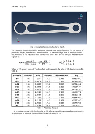
These change in dimensions are applied to the geometry. An example of the changed geometry is given
in Fig 6.
d d1 d2 d3
0 8 3 36
0.1 9 2.8 35.1
0.2 10 2.6 34.2
0.3 11 2.4 33.3
0.4 12 2.2 32.4
0.5 13 2 31.5
0.6 14 1.8 30.6
0.7 15 1.6 29.7
0.8 16 1.4 28.8
0.9 17 1.2 27.9
1 18 1 27

7. EML 5526 – Project 2 Ravishankar Venkatasubramanian
7
Fig. 6: Example of dimensionally altered sketch.
The change in dimensions provides a changed value of stress and deformation. For the purpose of
parametric analysis, mass has also been calculated. The optimum design must be able to withstand a
maximum load of 240 MPa and it must also have the lowest mass. For this analysis, the formula used
is given as:
Where α=100 (penalty number). This formula is used to calculate the value of f(d), data is presented in
Table 4.
Parameter Initial Mass Mass Stress Max Displacement max f(d)
d=0 2.31 1.5649 475.1 0.3483 98.63577922
d=0.1 2.31 1.68001 430.7 0.2867 80.18561039
d=0.2 2.31 1.78836 397.8 0.2445 66.52418182
d=0.3 2.31 1.88973 358.2 0.2125 50.06806494
d=0.4 2.31 1.98409 317.4 0.1888 33.10891342
d=0.5 2.31 2.07148 282.2 0.1708 18.48007792
d=0.6 2.31 2.15187 244.8 0.1577 2.931545455
d=0.7 2.31 2.22526 211.7 0.1477 0.963316017
d=0.8 2.31 2.29169 191.7 0.1408 0.992073593
d=0.9 2.31 2.35109 175.1 0.1357 1.017787879
d=1 2.31 2.40348 160.7 0.1321 1.040467532
Table 4: Parametric Analysis
It can be noticed from the table that the value of f(d) reduces from a high value to a low value and then
increases again. A graphical representation of f(d) vs d is shown in Fig 7.

8. EML 5526 – Project 2 Ravishankar Venkatasubramanian
8
Fig 7: Plot of f(d) vs d
The plot of f(d) vs d shows that the value of dopt might exist between d=0.7 and d=0.8. From the graph,
it can be told that the minimum is at d=0.79. Hence, we take dopt=0.79. Therefore, the dimensions vary:
d1= 10d + 8 = 15.9
d2 = -2d + 3 = 1.42
d3 = -9d + 36 = 28.89.
Substituting these dimensions back into the drawing, we obtain the value of stress, deformation and
mass. They are represented in Fig 8 and Fig 9.
Fig 8: Stress obtained in Optimum design case
-20
0
20
40
60
80
100
120
0 0.2 0.4 0.6 0.8 1 1.2
f(d)
Value of d
f(d) vs Parameter d

9. EML 5526 – Project 2 Ravishankar Venkatasubramanian
9
Fig. 9: Displacement obtained in Optimum design case
Therefore, the optimum mass, maximum stress and maximum displacement are determined by running
analysis and finding out the design and the parameters of the optimum design are represented in Table
5.
Table 5: Optimum Design
The optimum design condition has been obtained and the problem has been solved.
Parameter d=0.79
d1 15.9
d2 1.42
d3 28.89
Initial Mass 2.31
Mass 2.28683
Stress Max 192.5
Displacement
max
0.1413