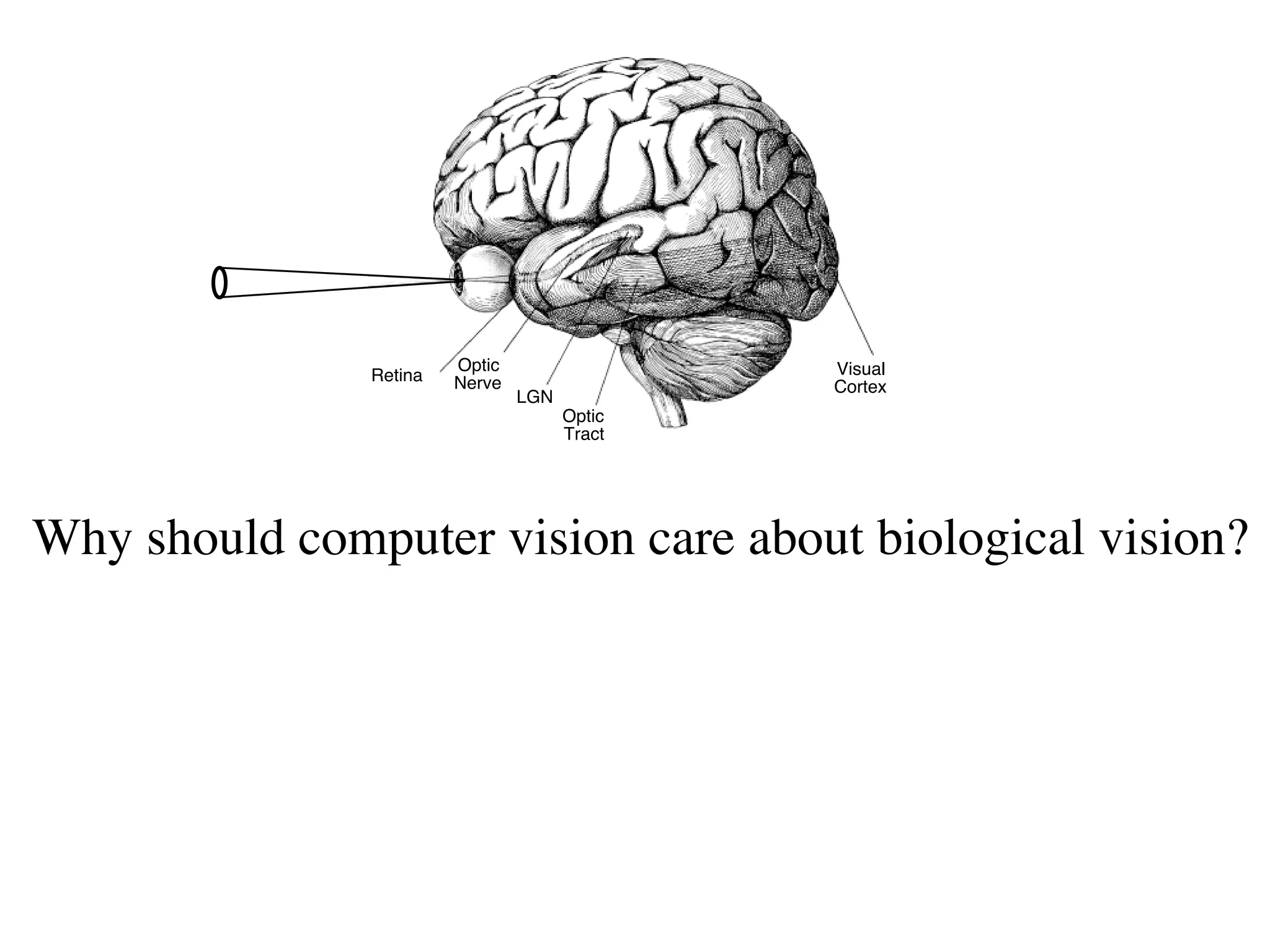
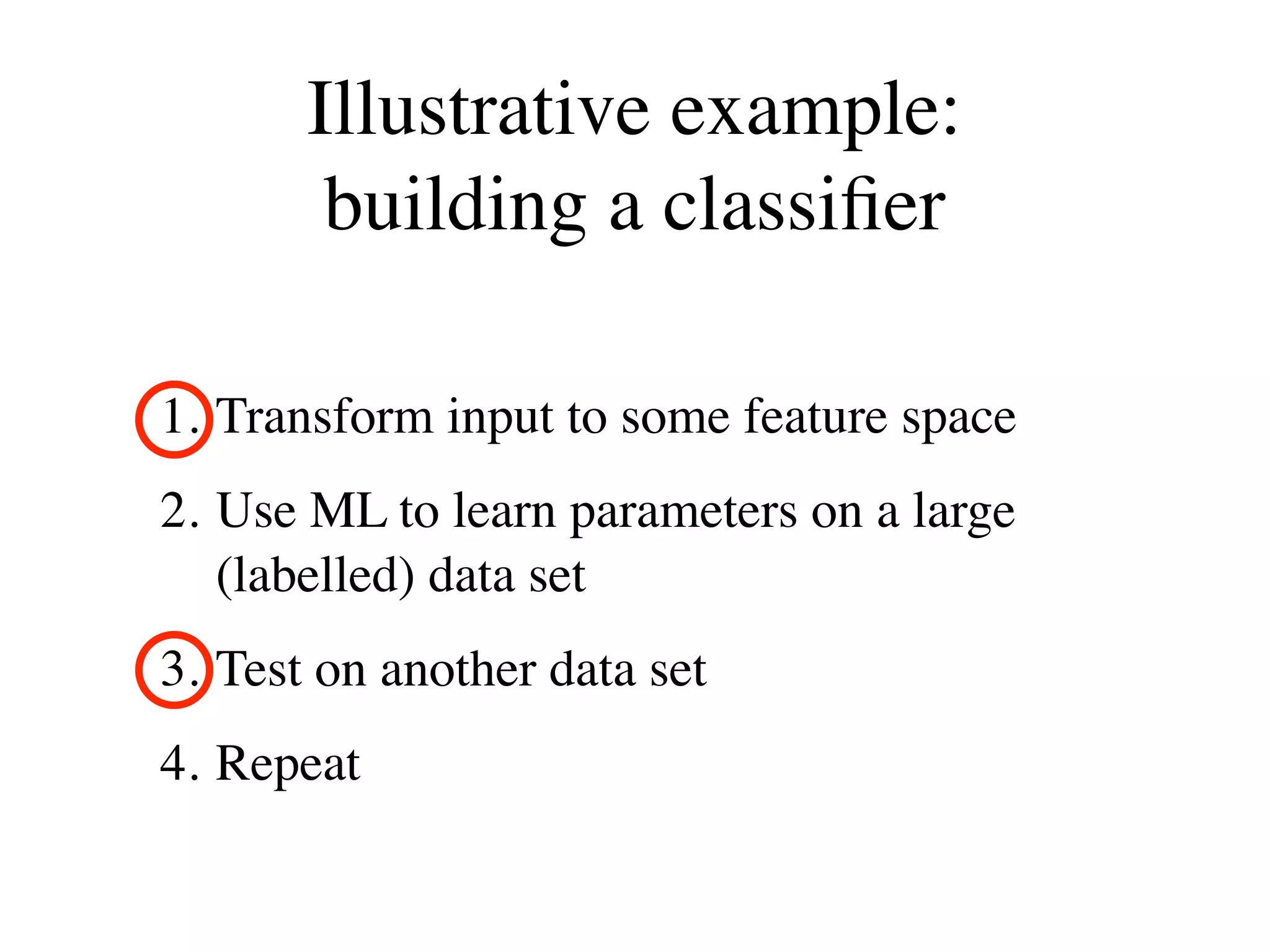
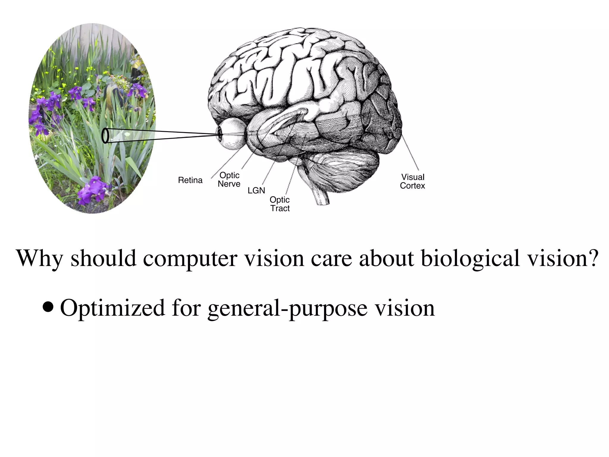
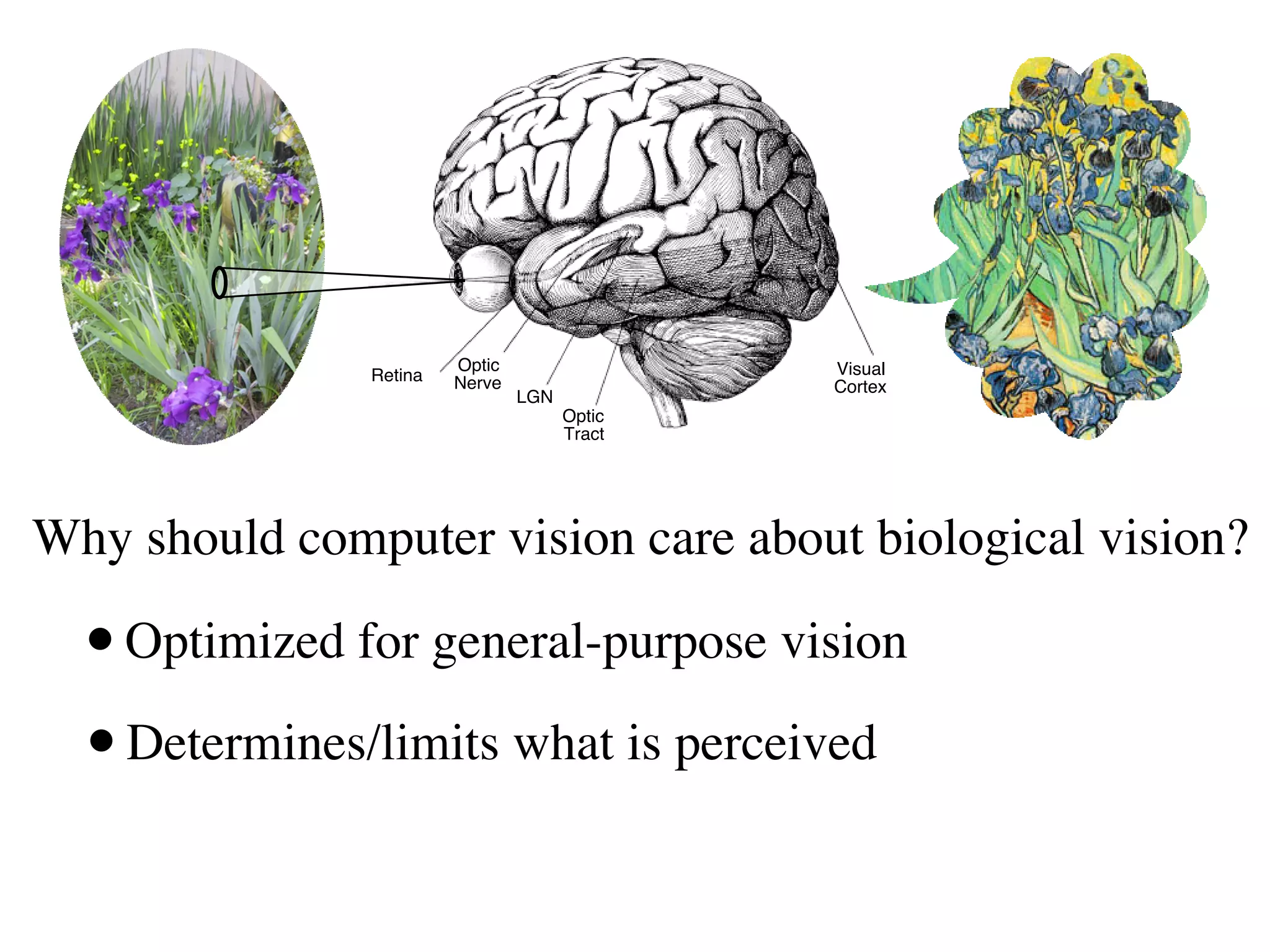
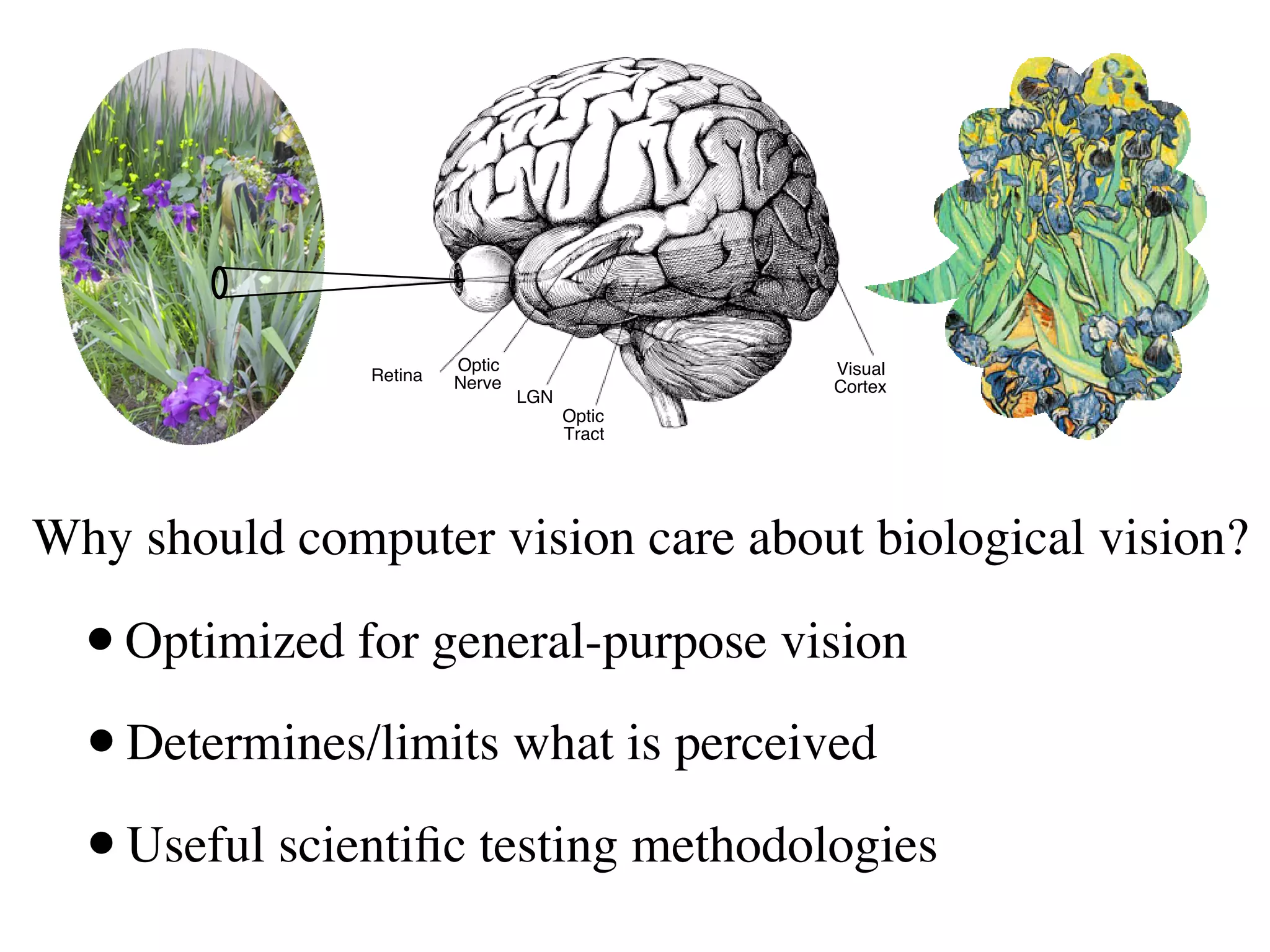
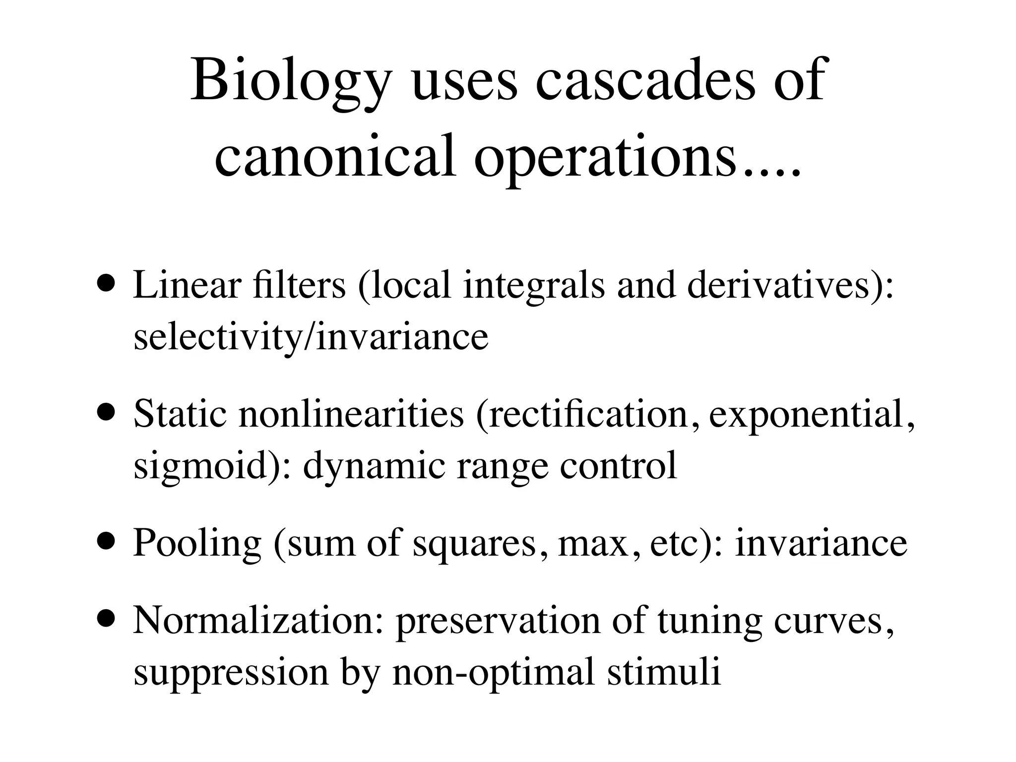
1. The document discusses using principles from biological vision to improve computer vision systems. 2. It describes how computer vision has incorporated ideas from visual neuroscience, such as using oriented filters inspired by V1 simple cells and implementing normalization models. 3. The document argues that biology uses cascades of canonical operations like linear filtering, nonlinearities, and pooling in an optimized way for general-purpose vision, and following these principles can improve computer vision tasks like object recognition.

1. Synthesis for understanding
and evaluating vision systems
Eero Simoncelli
Howard Hughes Medical Institute,
Center for Neural Science, and
Courant Institute of Mathematical Sciences
New York University
Frontiers in Computer Vision Workshop
MIT, 21-24 Aug 2011

2. Computer
graphics
Visual
Optics/imaging
perception
Computer
Image Visual
vision
processing neuroscience
Machine
Robotics
learning

3. Computer
graphics
Visual
Optics/imaging
perception
Computer
Image Visual
vision
processing neuroscience
Machine
Robotics
learning

4. Optic Visual
Retina Nerve Cortex
LGN
Optic
Tract
Why should computer vision care about biological vision?

5. Optic Visual
Retina Nerve Cortex
LGN
Optic
Tract
Why should computer vision care about biological vision?
• Optimized for general-purpose vision

6. Optic Visual
Retina Nerve Cortex
LGN
Optic
Tract
Why should computer vision care about biological vision?
• Optimized for general-purpose vision
• Determines/limits what is perceived

7. Optic Visual
Retina Nerve Cortex
LGN
Optic
Tract
Why should computer vision care about biological vision?
• Optimized for general-purpose vision
• Determines/limits what is perceived
• Useful scientific testing methodologies

8. Illustrative example:
building a classifier
1. Transform input to some feature space
2. Use ML to learn parameters on a large
(labelled) data set
3. Test on another data set
4. Repeat

9. Illustrative example:
building a classifier
1. Transform input to some feature space
2. Use ML to learn parameters on a large
(labelled) data set
3. Test on another data set
4. Repeat

10. Which features?
[Adelson & Bergen, 1985]

11. Which features?
Oriented filters: capture stimulus-dependency of neural
responses in primary visual cortex (area V1)
Simple cell
Complex cell +
[Adelson & Bergen, 1985]

12. Which features?
Oriented filters: capture stimulus-dependency of neural
responses in primary visual cortex (area V1)
Simple cell
Complex cell +
[Adelson & Bergen, 1985]

13. Which features?
Oriented filters: capture stimulus-dependency of neural
responses in primary visual cortex (area V1)
Simple cell
Complex cell +
[Adelson & Bergen, 1985]

14. Retinal image
The normalization model of simple cells
Firing
rate
Retinal image
Other cortical cells
RC circuit implementation
Firing
Retinal image rate
Other cortical cells
[Carandini, Heeger, and Movshon, 1996]

15. Retinal image
The normalization model of simple cells
Firing
rate
Retinal image
Other cortical cells
RC circuit implementation
Firing
Retinal image rate
Other cortical cells
[Carandini, Heeger, and Movshon, 1996]

16. Dynamic retina/LGN model
[Mante, Bonin & Carandini 2008]

17. 2-stage MT model
Input: image intensities Input: V1 afferents
1
Linear
Receptive ... ...
Field
Half-squaring ...
Rectification ... 2 2
1
+ +
Divisive ... ...
Normalization
Output: V1 neurons tuned for Output: MT neurons tuned for
spatio-temporal orientation local image velocity
[Simoncelli & Heeger, 1998]

18. 2-stage MT model
Input: image intensities Input: V1 afferents
1
Linear
Receptive ... ...
Field
Half-squaring ...
Rectification ... 2 2
1
+ +
Divisive ... ...
Normalization
Output: V1 neurons tuned for Output: MT neurons tuned for
spatio-temporal orientation local image velocity
[Simoncelli & Heeger, 1998]

19. Biology uses cascades of
canonical operations....
• Linear filters (local integrals and derivatives):
selectivity/invariance
• Static nonlinearities (rectification, exponential,
sigmoid): dynamic range control
• Pooling (sum of squares, max, etc): invariance
• Normalization: preservation of tuning curves,
suppression by non-optimal stimuli

20. Improved object recognition?
“In many recent object recognition systems, feature extraction
stages are generally composed of a filter bank, a non-linear
transformation, and some sort of feature pooling layer [...]
We show that using non-linearities that include rectification
and local contrast normalization is the single most important
ingredient for good accuracy on object recognition
benchmarks. We show that two stages of feature extraction
yield better accuracy than one....”
- From the abstract of
“What is the Best Multi-Stage Architecture for Object Recognition?”
Kevin Jarrett, Koray Kavukcuoglu, Marc’Aurelio Ranzato and Yann LeCun
ICCV-2009

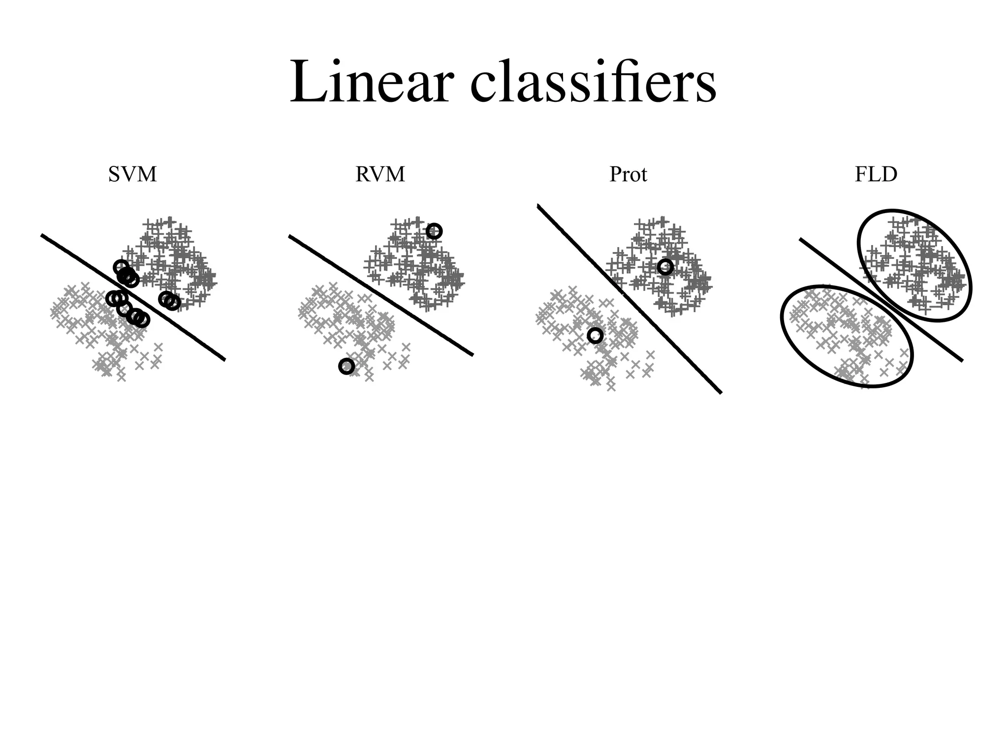
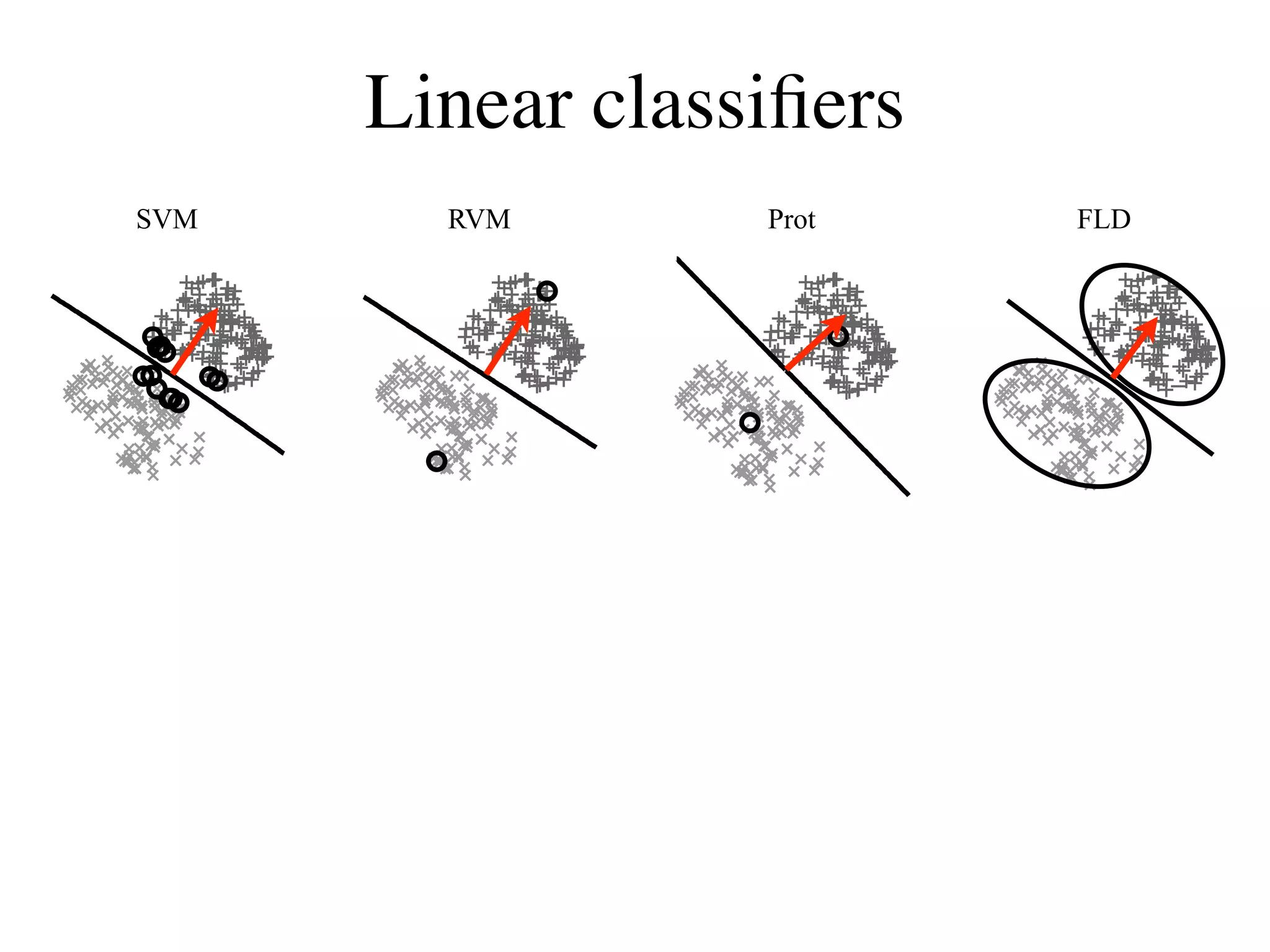
21. Using synthesis to test models I:
Gender classification
• 200 face images (100 male, 100 female)
• Labeled by 27 human subjects
• Four linear classifiers trained on subject data
[Graf & Wichmann, NIPS*03]

22. Linear classifiers
SVM RVM Prot FLD

23. Linear classifiers
SVM RVM Prot FLD

24. Linear classifiers
SVM RVM Prot FLD
SVM RVM Prot FLD trained
on
! true
W data
classifier vectors may be visualized as images:
! subj
W data

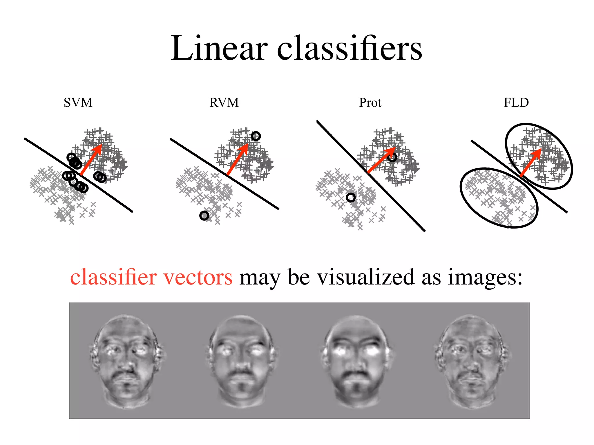
25. Validation by “gender-morphing”
Subtract classifier Add classifier
!=−21 !=−14 !=−7 !=0 !=7 !=14 !=21
SVM
RVM
Prot
FLD
[Wichmann, Graf, Simoncelli, Bülthoff, Schölkopf, NIPS*04]

26. Human subject responses
Perceptual validation
100
SVM
RVM
% Correct
Proto
FLD
50
0.25 0.5 1.0 2.0 4.0 8.0
Amount of classifier image added/subtracted
(arbitrary units)
[Wichmann, Graf, Simoncelli, Bülthoff, Schölkopf, NIPS*04]

27. rates of an IT population of 200 neurons, despite variation evidence suggests that the ventral stream transfor
in object position and size [19]. It is important to note that (culminating in IT) solves object recognition by unta
Using synthesis to test models II:
using ‘stronger’ (e.g. non-linear) classifiers did not substan-
tially improve recognition performance and the same
object manifolds. For each visual image striking the e
total transformation happens progressively (i.e. st
Ventral stream
representation
[DiCarlo Cox, 2007]

28. F
a re
fie
V4 fie
Receptive field size (deg)
25 V2 V
20 (1
ec
15 d
10
(b
V1
si
5 T
o
0
b
0 5 10 15 20 25 30 35 40 45 50 et
Eccentricity, receptive center (deg)
Receptive field field center (deg) ec
la
b [Gattass et. al., 1981;
o
Gattass et. al., 1988] th

29. V1 V4
V2
IT
V1 V2 V4 IT
[Freeman Simoncelli, Nature Neurosci, Sep 2011]

30. 2
1
1
Canonical computation Ventral stream
“complex” cell
Ventral stream
V1 cells
receptive fields
+
[Freeman Simoncelli, Nature Neurosci, Sep 2011]

31. 2
1
1
Canonical computation Ventral stream
“complex” cell
Ventral stream
V1 cells
receptive fields
3.1
1.4
+ 12.5
.
.
.
[Freeman Simoncelli, Nature Neurosci, Sep 2011]

32. 2
1
1
Canonical computation Ventral stream
“complex” cell
Ventral stream
V1 cells
receptive fields
3.1
1.4
+ 12.5
.
.
.
How do we test this?
[Freeman Simoncelli, Nature Neurosci, Sep 2011]

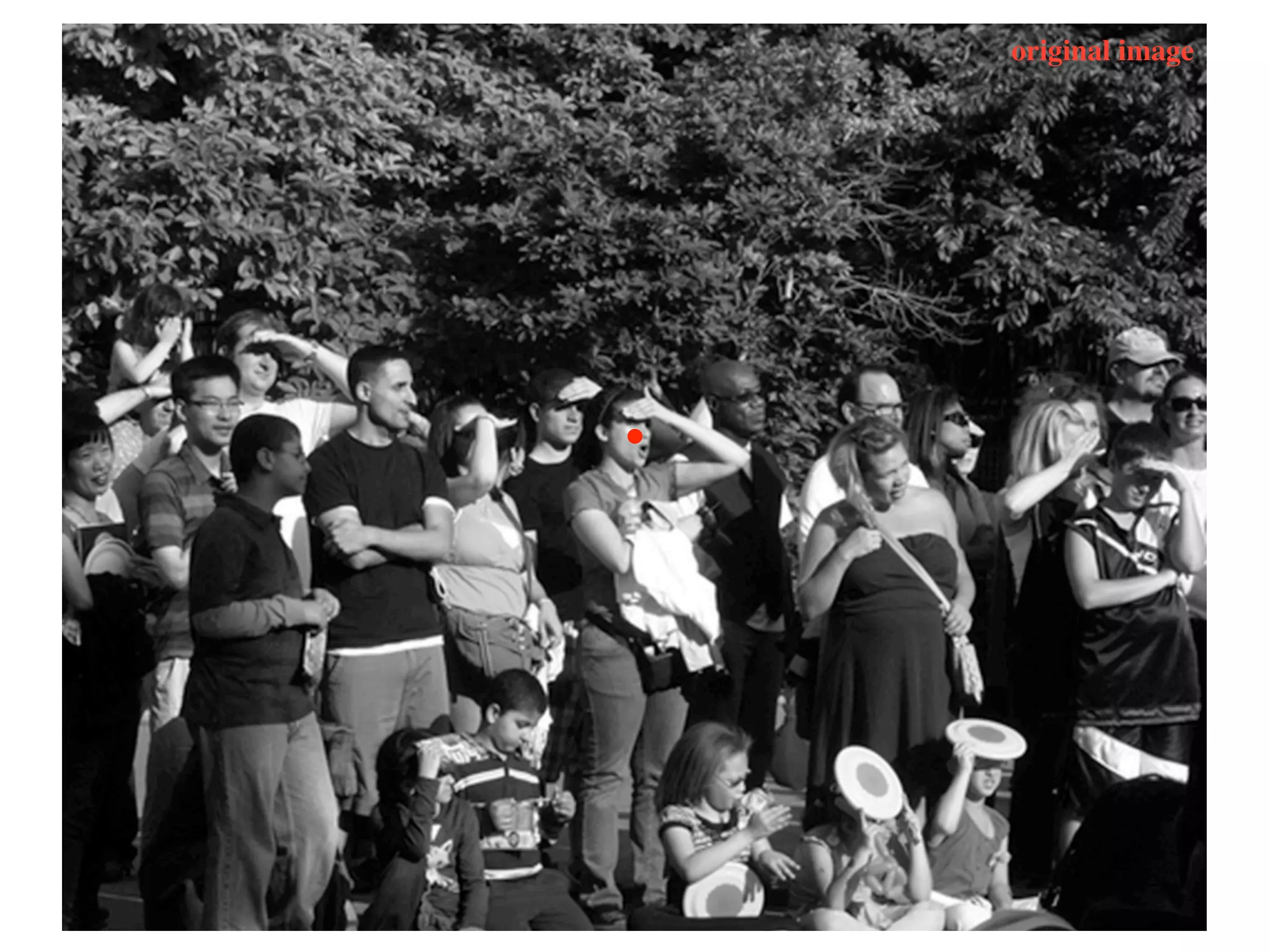
33. Model
model
Original image responses model
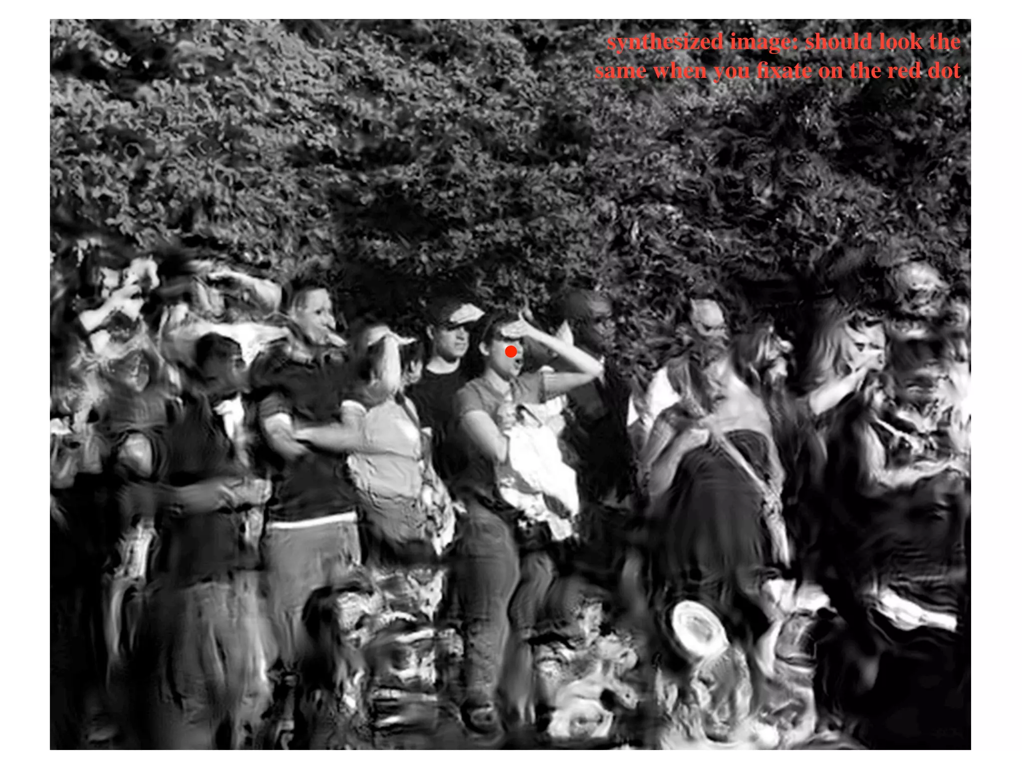
Synthesized image
3.1
1.4
12.5
.
. 250
.
150
25
170
40
Idea: synthesize random samples from the equivalence
class of images with identical model responses
Scientific prediction: such images should look the same
(“Metamers”)
[Freeman Simoncelli, Nature Neurosci, Sep 2011]

34. Model
Original image responses Synthesized image
3.1
1.4
12.5
.
.
.
Idea: synthesize random samples from the equivalence
class of images with identical model responses
Scientific prediction: such images should look the same
(“Metamers”)
[Freeman Simoncelli, Nature Neurosci, Sep 2011]

35. Model
Original image responses Synthesized image
3.1
1.4
12.5
.
.
.
Idea: synthesize random samples from the equivalence
class of images with identical model responses
Scientific prediction: such images should look the same
(“Metamers”)
[Freeman Simoncelli, Nature Neurosci, Sep 2011]

36. original image

38. synthesized image: should look the
same when you fixate on the red dot

39. Reading
a
b
[Freeman Simoncelli, Nature Neurosci, Sep 2011]

40. Camouflage
c
[Freeman Simoncelli, Nature Neurosci, Sep 2011]

41. Cascades of linear filtering, squaring/products,
averaging over local regions....

42. Cascades of linear filtering, squaring/products,
averaging over local regions....
Can this really lead to object recognition?

43. Cascades of linear filtering, squaring/products,
averaging over local regions....
Can this really lead to object recognition?
“Perhaps texture, somewhat redefined, is the
primitive stuff out of which form is
constructed”
- Jerome Lettvin, 1976