Downloaded 2,223 times
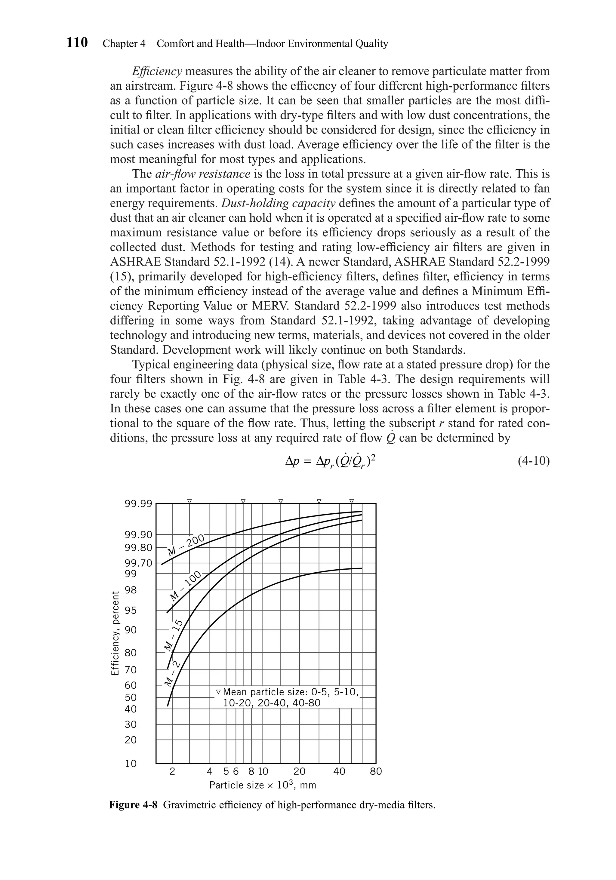
1 1
1-2 Common HVAC Units and Dimensions 5
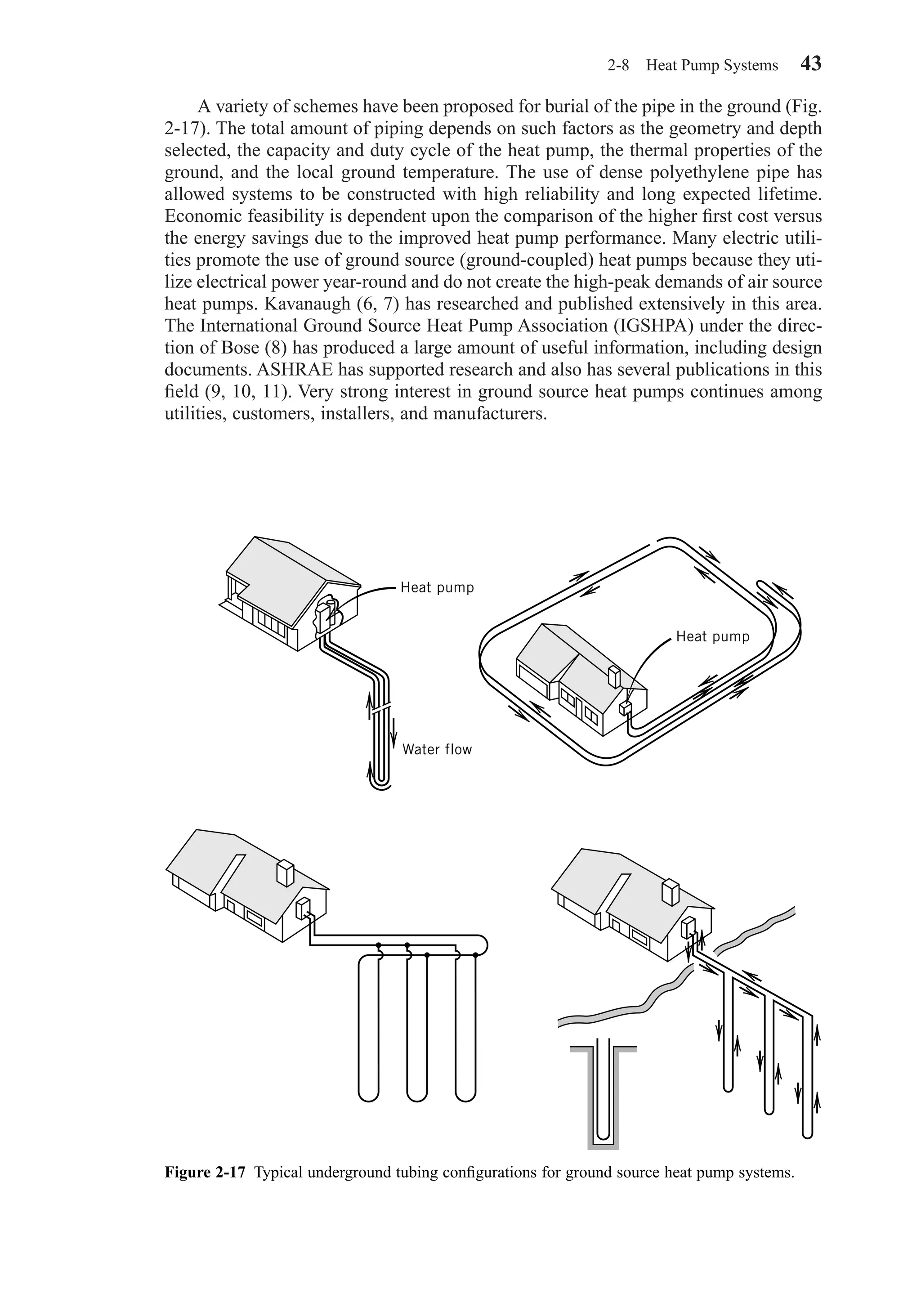
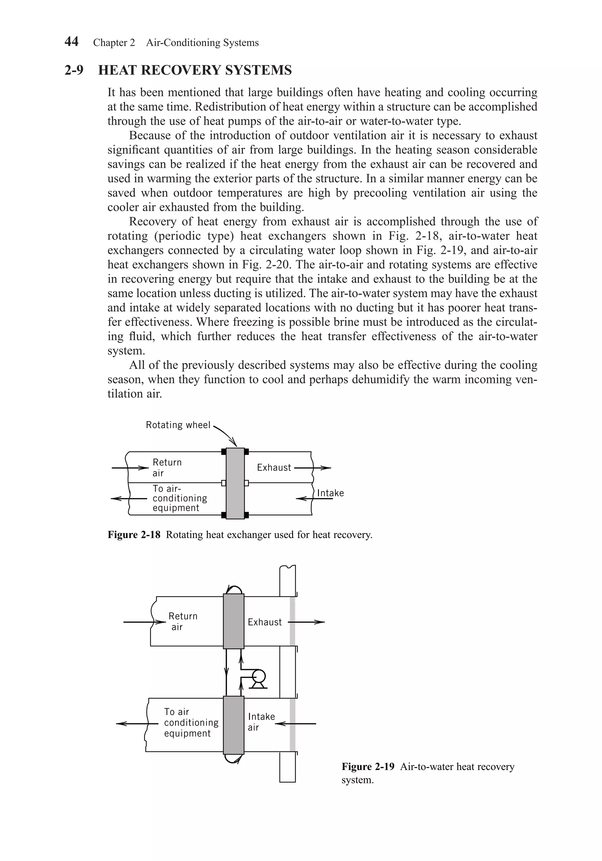
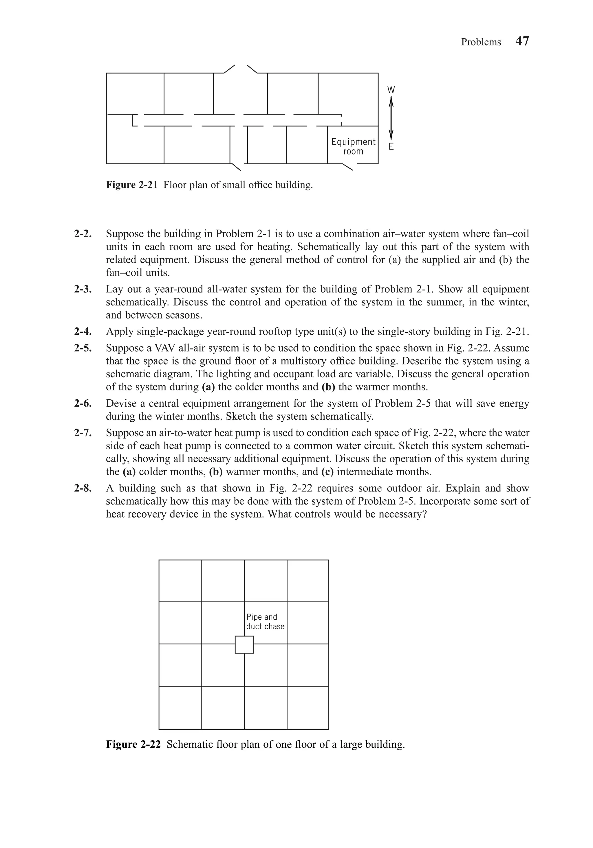
Chapter01.qxd 6/15/04 2:32 PM Page 5](https://image.slidesharecdn.com/fayec-160521192803/75/Faye-c-mc_quiston_-_jerald_d-_parker_-_jeffrey_d-22-2048.jpg)
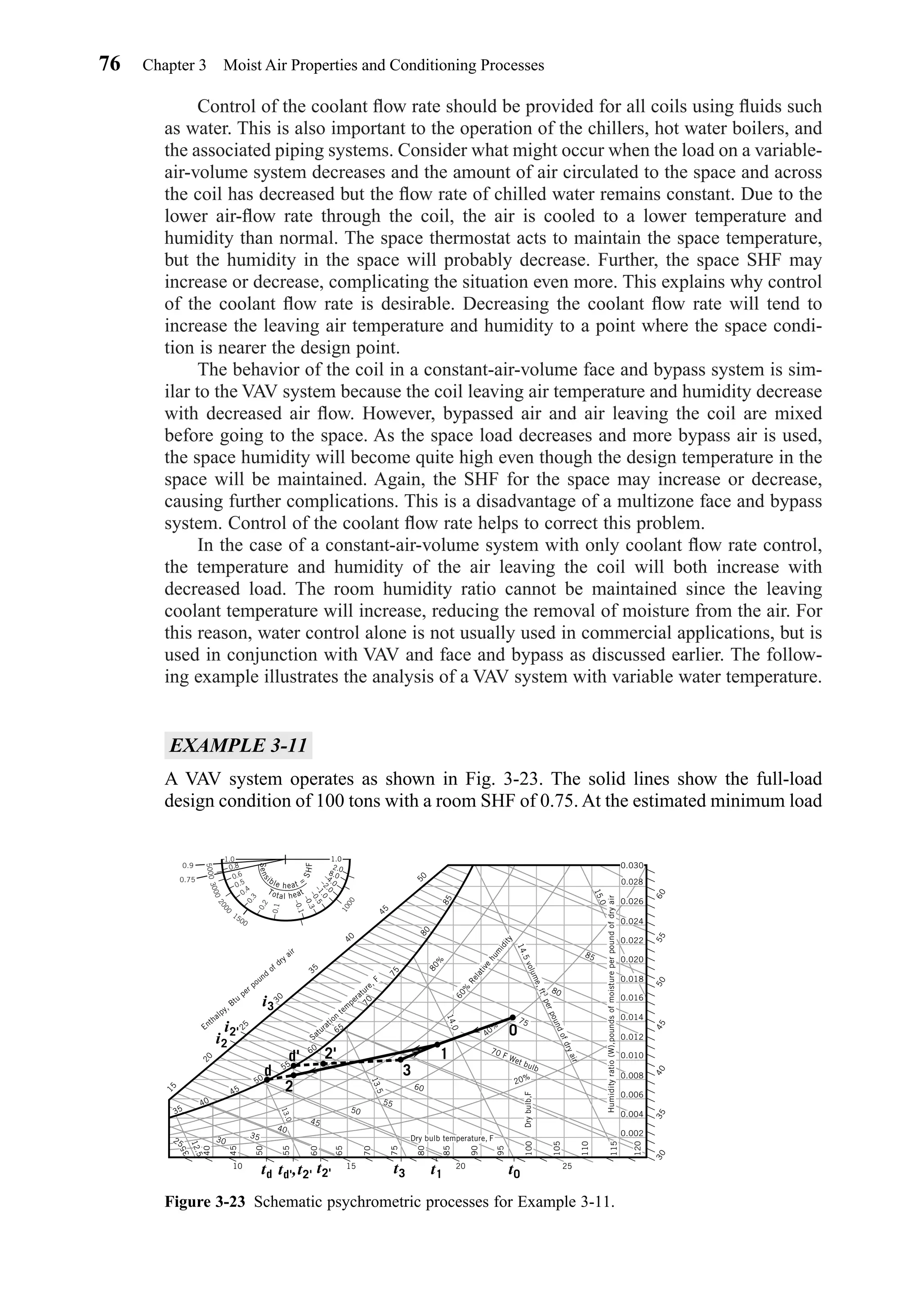
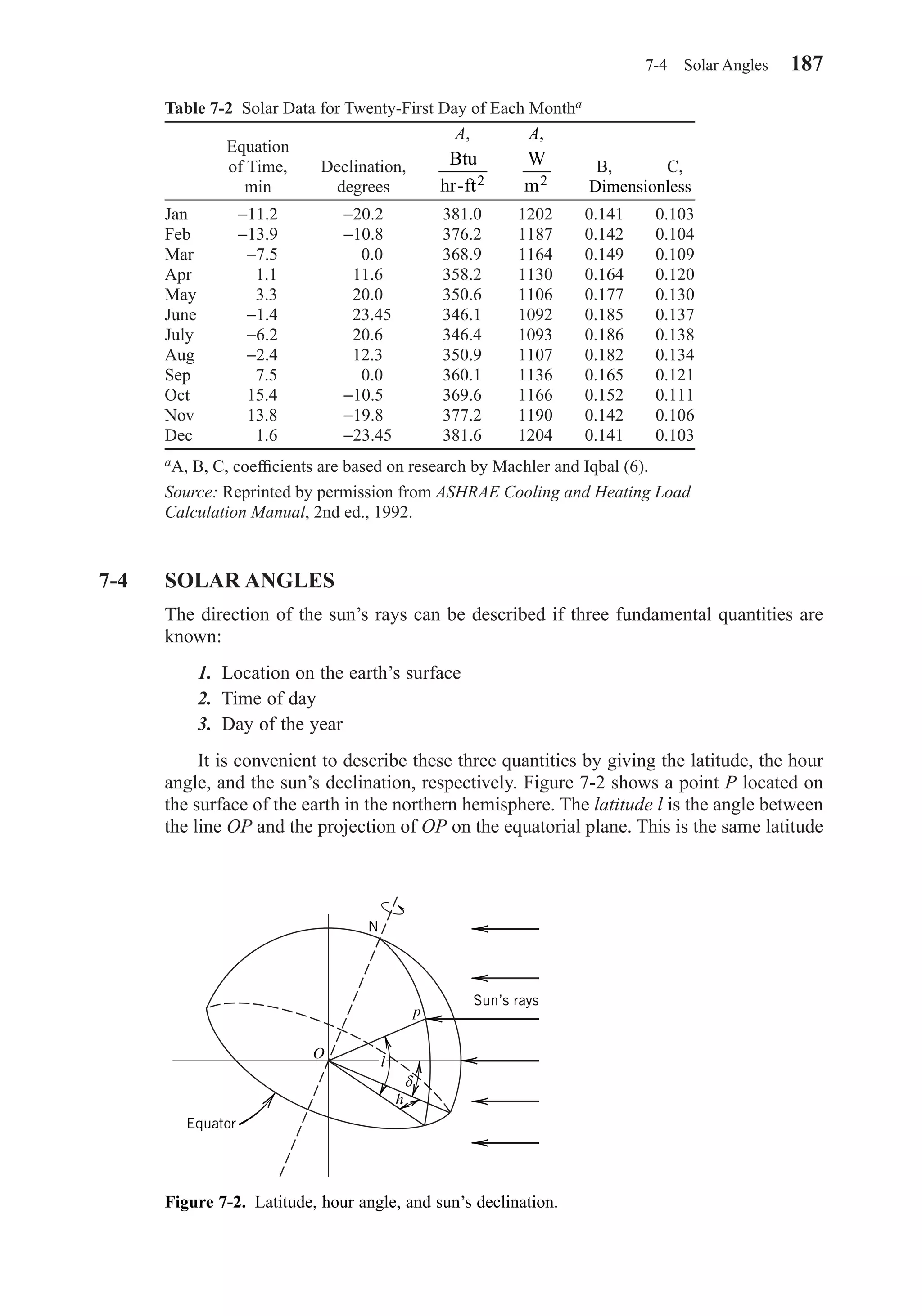
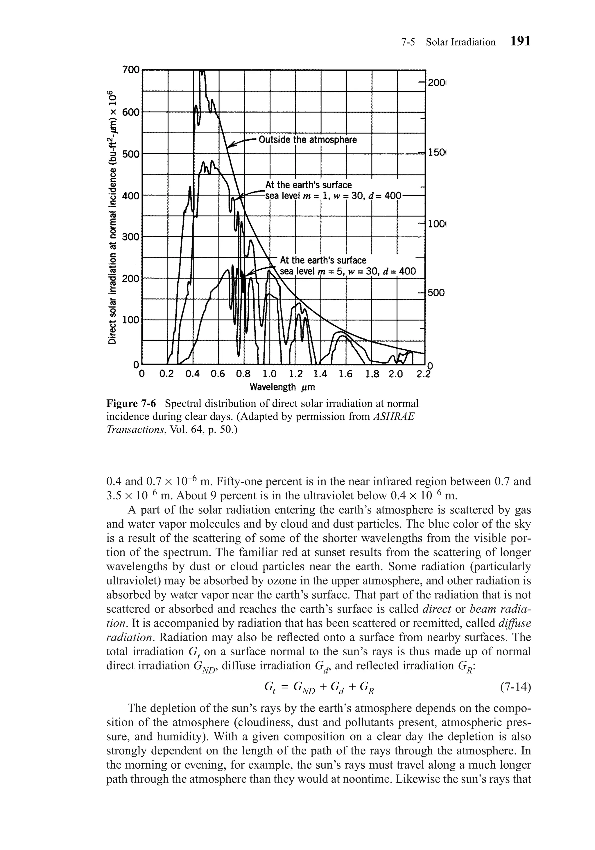
![EXAMPLE 1-2
Proposed improvements to a heating system are estimated to cost $8000 and should
result in an annual savings to the owner of $720 over the 15-year life of the equip-
ment. The interest rate used for making the calculation is 9 percent per year and sav-
ings are assumed to occur uniformly at the end of each month as the utility bill is paid.
SOLUTION
Using Eq. 1-1 and noting that the savings is assumed to be $60 per month, the pres-
ent worth of the savings is computed.
P = ($60) [1 − (1 + (0.09/12))−(15)(12)] / (0.09/12)
P = $5916 < $8000
Since the present worth of the savings is less than the first cost, the proposed project
is not feasible. This is true even though the total savings over the entire 15 years is
($720)(15) = $10,800, more than the first cost in actual dollars. Dollars in the future
are worth less than dollars in the present. Notice that with a lower interest rate or
longer equipment life the project might have become feasible. Computations of this
type are important to businesses in making decisions about the expenditure of money.
Sometimes less obvious factors, such as increased productivity of workers due to
improved comfort, may have to be taken into account.
1-3 FUNDAMENTAL PHYSICAL CONCEPTS
Good preparation for a study of HVAC system design most certainly includes courses
in thermodynamics, fluid mechanics, heat transfer, and system dynamics. The first law
of thermodynamics leads to the important concept of the energy balance. In some
cases the balance will be on a closed system or fixed mass. Often the energy balance
will involve a control volume, with a balance on the mass flowing in and out consid-
ered along with the energy flow.
The principles of fluid mechanics, especially those dealing with the behavior of
liquids and gases flowing in pipes and ducts, furnish important tools. The economic
tradeoff in the relationship between flow rate and pressure loss will often be inter-
twined with the thermodynamic and heat transfer concepts. Behavior of individual
components or elements will be expanded to the study of complete fluid distribution
systems. Most problems will be presented and analyzed as steady-flow and steady-
state even though changes in flow rates and properties frequently occur in real sys-
tems. Where transient or dynamic effects are important, the computations are often
complex, and computer routines are usually used.
Some terminology is unique to HVAC applications, and certain terms have a spe-
cial meaning within the industry. This text will identify many of these special terms.
Those and others are defined in the ASHRAE Terminology of HVACR (14). Some of
the more important processes, components, and simplified systems required to main-
tain desired environmental conditions in spaces will be described briefly.
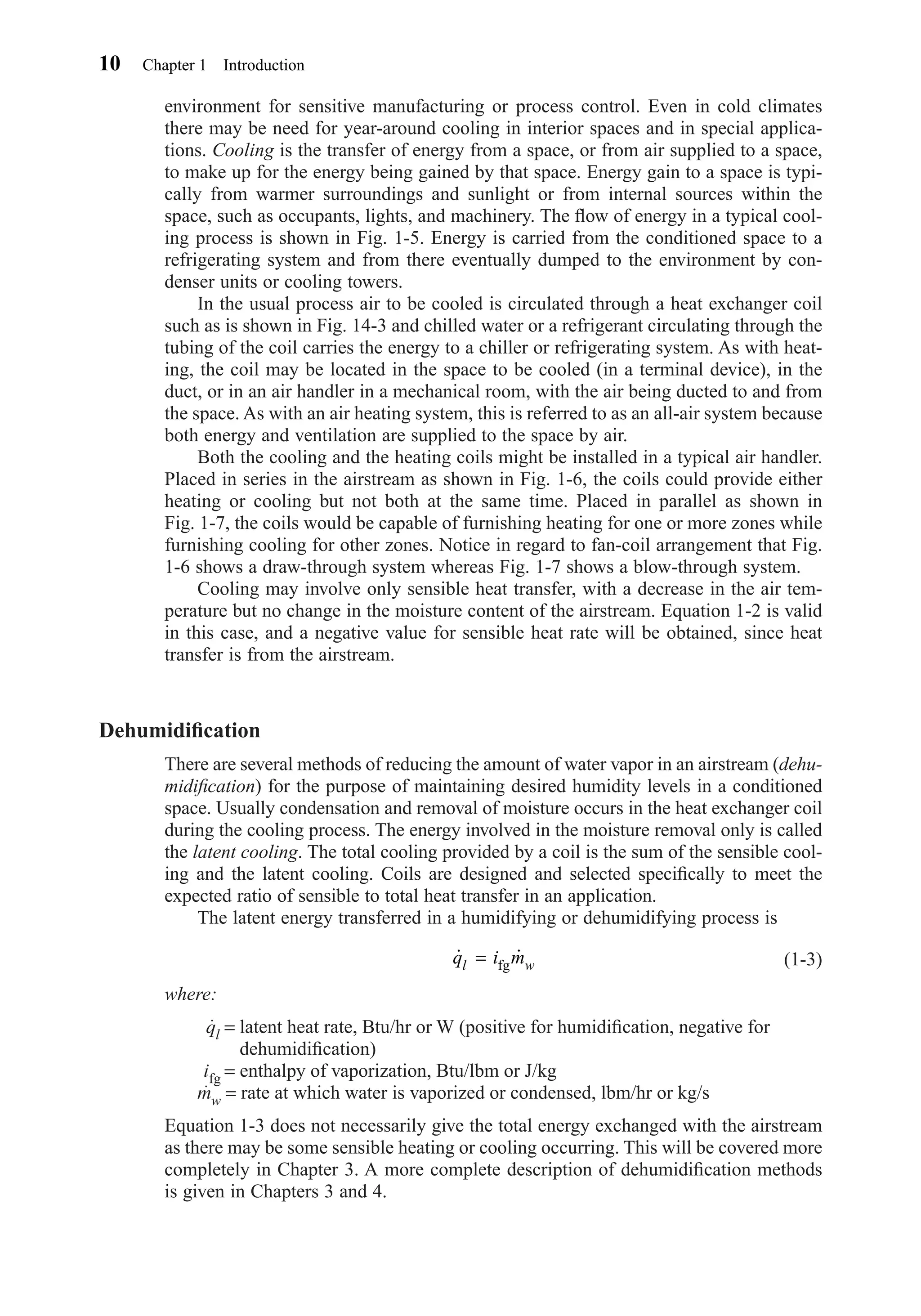
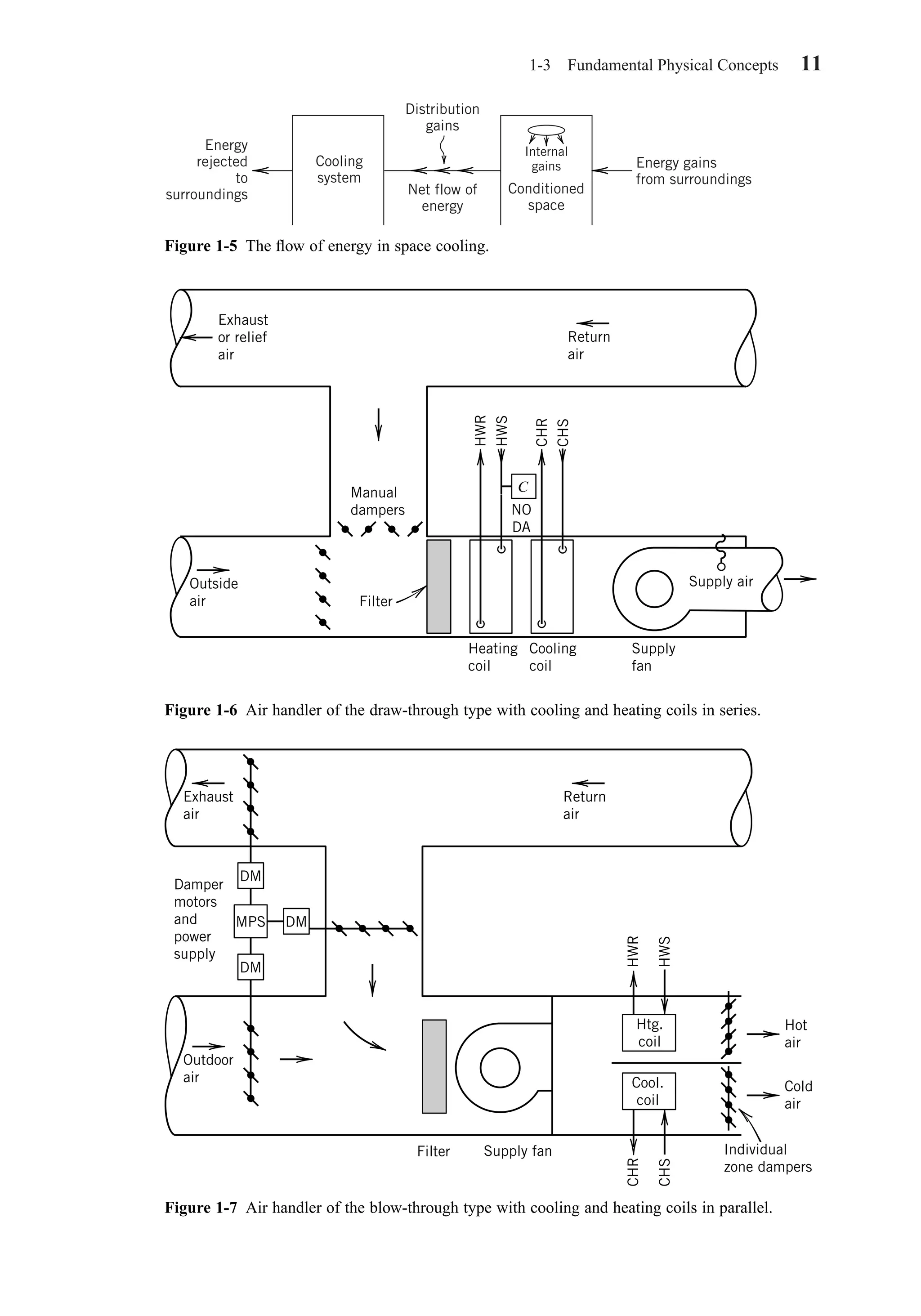
Heating
In space conditioning, heating is performed either (a) to bring a space up to a higher
temperature than existed previously, for example from an unoccupied nighttime
6 Chapter 1 Introduction
Chapter01.qxd 6/15/04 2:32 PM Page 6](https://image.slidesharecdn.com/fayec-160521192803/75/Faye-c-mc_quiston_-_jerald_d-_parker_-_jeffrey_d-23-2048.jpg)


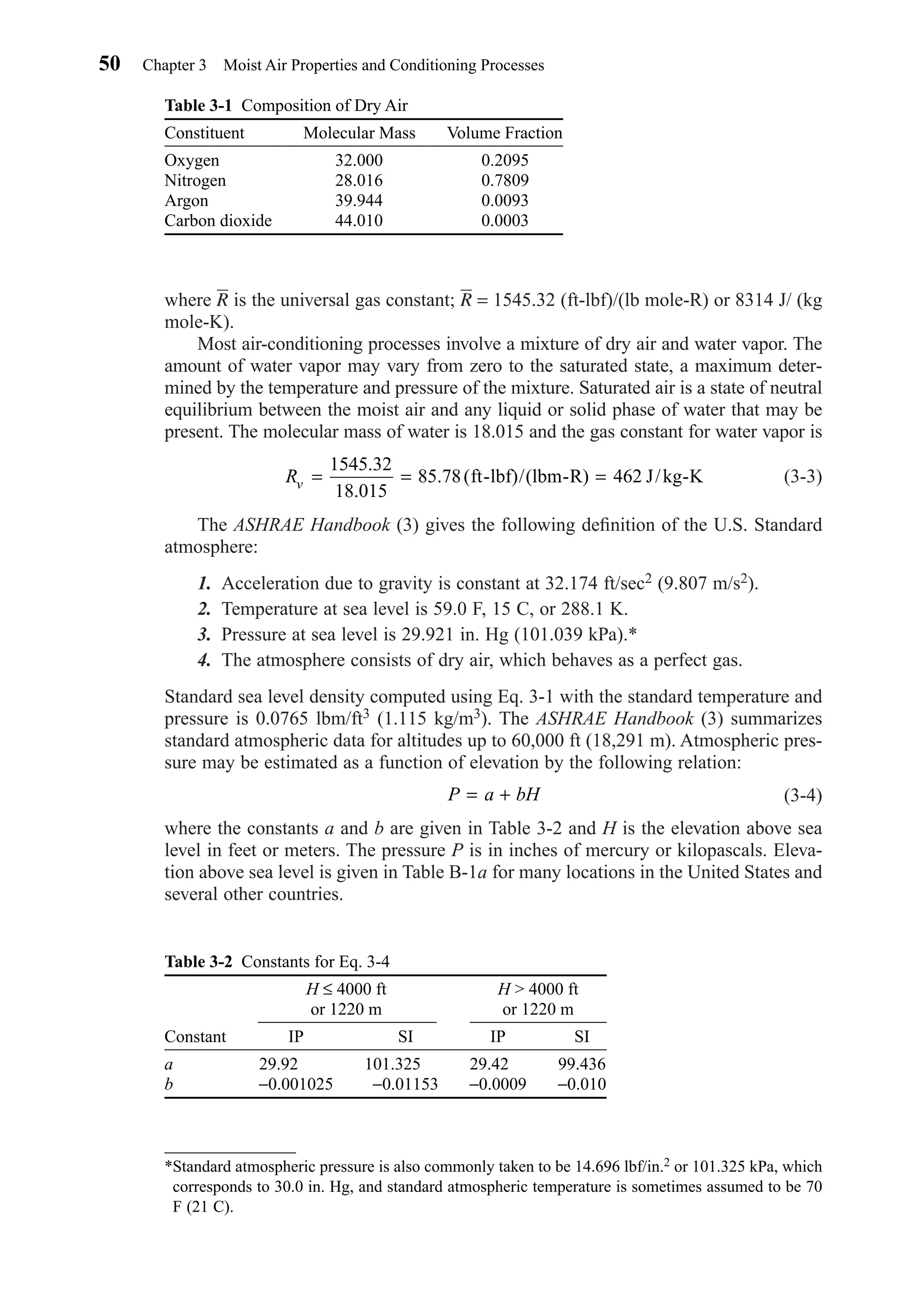
![3-2 FUNDAMENTAL PARAMETERS
Moist air up to about three atmospheres pressure obeys the perfect gas law with suf-
ficient accuracy for most engineering calculations. The Dalton law for a mixture of
perfect gases states that the mixture pressure is equal to the sum of the partial pres-
sures of the constituents:
(3-5)
For moist air
(3-6)
Because the various constituents of the dry air may be considered to be one gas, it fol-
lows that the total pressure of moist air is the sum of the partial pressures of the dry
air and the water vapor:
(3-7)
Each constituent in a mixture of perfect gases behaves as if the others were not pres-
ent. To compare values for moist air assuming ideal gas behavior with actual table val-
ues, consider a saturated mixture of air and water vapor at 80 F. Table A-1a gives the
saturation pressure ps of water as 0.507 lbf/in.2. For saturated air this is the partial
pressure pv of the vapor. The mass density is 1/v = 1/632.67 or 0.00158 lbm/ft3. By
using Eq. 3-1 we get
This result is accurate within about 0.25 percent. For nonsaturated conditions water
vapor is superheated and the agreement is better. Several useful terms are defined
below.
The humidity ratio W is the ratio of the mass mv of the water vapor to the mass
ma of the dry air in the mixture:
(3-8)
The relative humidity φ is the ratio of the mole fraction of the water vapor xv in a
mixture to the mole fraction xs of the water vapor in a saturated mixture at the same
temperature and pressure:
(3-9)
For a mixture of perfect gases, the mole fraction is equal to the partial pressure ratio
of each constituent. The mole fraction of the water vapor is
(3-10)
Using Eq. 3-9 and letting ps stand for the partial pressure of the water vapor in a sat-
urated mixture, we may express the relative humidity as
(3-11)
Since the temperature of the dry air and the water vapor are assumed to be the same
in the mixture,
(3-12)φ
ρ
ρ= = [ ]
p
p
t P
v RvT
s RvT
v
s
/
/ ,
φ = =
p
p
p
p
v P
s P
v
s
/
/
xv
p
P
v
=
φ = [ ]x
x
t P
v
s ,
W
m
m
v
a
=
1 0 507 144
85 78 459 67 80
0 001577
v
P
v
R
v
T
= = =
+
=ρ
. ( )
. ( . )
. lbm/ft3
P p pa v= +
P p p p p pv= + + + +N O CO Ar2 2 2
P p p p1 2 3= + +
3-2 Fundamental Parameters 51
Chapter03.qxd 6/15/04 2:31 PM Page 51](https://image.slidesharecdn.com/fayec-160521192803/75/Faye-c-mc_quiston_-_jerald_d-_parker_-_jeffrey_d-68-2048.jpg)
![where the densities ρv and ρs are referred to as the absolute humidities of the water
vapor (mass of water per unit volume of mixture). Values of ρs may be obtained from
Table A-1a.
Using the perfect gas law, we can derive a relation between the relative humidity
φ and the humidity ratio W:
(3-13a)
and
(3-13b)
and
(3-14a)
For the air–water vapor mixture, Eq. 3-14a reduces to
(3-14b)
Combining Eqs. 3-11 and 3-14b gives
(3-15)
The degree of saturation µ is the ratio of the humidity ratio W to the humidity
ratio Ws of a saturated mixture at the same temperature and pressure:
(3-16)
The dew point td is the temperature of saturated moist air at the same pressure and
humidity ratio as the given mixture. As a mixture is cooled at constant pressure, the
temperature at which condensation first begins is the dew point. At a given mixture
(total) pressure, the dew point is fixed by the humidity ratio W or by the partial pres-
sure of the water vapor. Thus td, W, and pv are not independent properties.
The enthalpy i of a mixture of perfect gases is equal to the sum of the enthalpies
of each constituent,
(3-17)
and for the air–water vapor mixture is usually referenced to the mass of dry air. This
is because the amount of water vapor may vary during some processes but the amount
of dry air typically remains constant. Each term in Eq. 3-17 has the units of energy
per unit mass of dry air. With the assumption of perfect gas behavior, the enthalpy is
a function of temperature only. If 0 F or 0 C is selected as the reference state where
the enthalpy of dry air is 0, and if the specific heats cpa and cpv are assumed to be con-
stant, simple relations result:
(3-18)
(3-19)
where the enthalpy of saturated water vapor ig at 0 F is 1061.2 Btu/lbm and 2501.3
kJ/kg at 0 C.
i i c tv g pv= +
i c ta pa=
i i Wia v= +
µ = [ ]W
W
t Ps ,
φ =
Wp
p
a
s0 6219.
W
p
p
p
p
v
a
v
a
= =
18 015
28 965
0 6219
.
.
.
W
M p
M p
v v
a a
=
ma
p V
R T
p VM
RT
a
a
a a
= =
mv
p V
R T
p VM
RT
v
v
v v
= =
52 Chapter 3 Moist Air Properties and Conditioning Processes
Chapter03.qxd 6/15/04 2:31 PM Page 52](https://image.slidesharecdn.com/fayec-160521192803/75/Faye-c-mc_quiston_-_jerald_d-_parker_-_jeffrey_d-69-2048.jpg)
![Using Eqs. 3-17, 3-18, and 3-19 with cpa and cpv taken as 0.240 and 0.444 Btu/
(lbm-F), respectively, we have
(3-20a)
In SI units, Eq. 3-20a becomes
(3-20b)
where cpa and cpv are 1.0 and 1.86 kJ/(kg-C), respectively.
EXAMPLE 3-1
Compute the enthalpy of saturated air at 60 F and standard atmospheric pressure.
SOLUTION
Equation 3-20a will be used to compute enthalpy; however, the humidity ratio Ws must
first be determined from Eq. 3-14b:
From Table A-1a, ps = 0.2563 psia and
The enthalpy calculated using ideal gas relations is about 0.25 percent low but quite
satisfactory for engineering calculations.
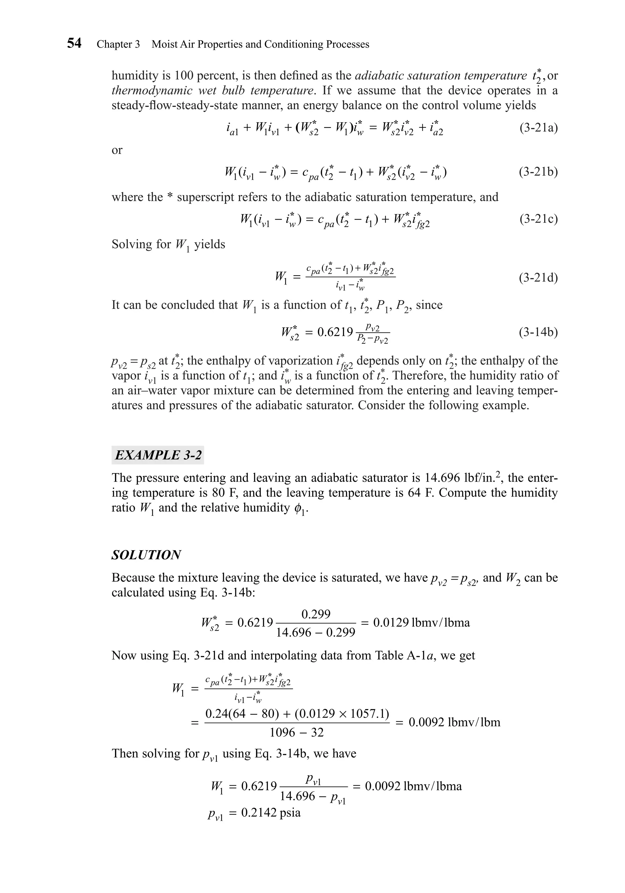
3-3 ADIABATIC SATURATION
The equations discussed in the previous section show that at a given pressure and dry
bulb temperature of an air–water vapor mixture, one additional property is required to
completely specify the state, except at saturation. Any of the parameters discussed (φ,
W, or i) would be acceptable; however, there is no practical way to measure any of
them. The concept of adiabatic saturation provides a convenient solution.
Consider the device shown in Fig. 3-1. The apparatus is assumed to operate so
that the air leaving at point 2 is saturated. The temperature t2, where the relative
W
i
s
s
=
−
=
= + +[ ] =
0 6219
0 2563
14 696 0 2563
0 01104
0 24 60 0 01104 1061 2 0 444 60 26 41
.
.
. .
.
( . ) . . ( . ) .
lbmv/lbma
Btu/lbma
Ws
p
p
p
P p
s
a
s
s
= = −0 6219 0 6219. .
i t W t= + +1 0 2501 3 1 86. ( . . ) kJ/kga
i t W t= + +0 240 1061 2 0 444. ( . . ) Btu/lbma
3-3 Adiabatic Saturation 53
Figure 3-1 Schematic of adiabatic saturation device.
1 2
1,t1,P1,W1φ φt2,Ws2,P2, 2* *
t2
Insulated
Liquid
water at t2
Chapter03.qxd 6/15/04 2:31 PM Page 53](https://image.slidesharecdn.com/fayec-160521192803/75/Faye-c-mc_quiston_-_jerald_d-_parker_-_jeffrey_d-70-2048.jpg)
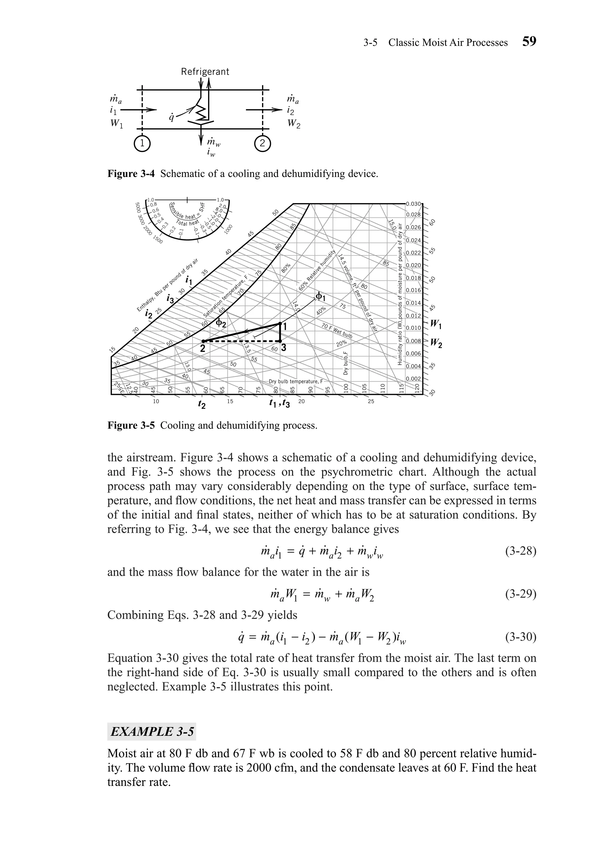
![SOLUTION
Equation 3-30 applies to this process, which is shown in Fig. 3-5. The following prop-
erties are read from Chart 1a: v1 = 13.85 ft3 lbma, i1 = 31.4 Btu/lbma, W1 = 0.0112
lbmv/lbma, i2 = 22.8 Btu/lbma, W2 = 0.0082 lbmv/lbma. The enthalpy of the conden-
sate is obtained from Table A-1a, iw = 28.08 Btu/lbmw. The mass flow rate ma is
obtained from Eq. 3-27:
Then
The last term, which represents the energy of the condensate, is seen to be small.
Neglecting the condensate term, q = 74,356 Btu/hr = 6.2 tons.
The cooling and dehumidifying process involves both sensible and latent heat
transfer; the sensible heat transfer rate is associated with the decrease in dry bulb tem-
perature, and the latent heat transfer rate is associated with the decrease in humidity
ratio. These quantities may be expressed as
(3-31)
and
(3-32)
By referring to Fig. 3-5 we may also express the latent heat transfer rate as
(3-33)
and the sensible heat transfer rate is given by
(3-34)
The energy of the condensate has been neglected. Obviously
(3-35)
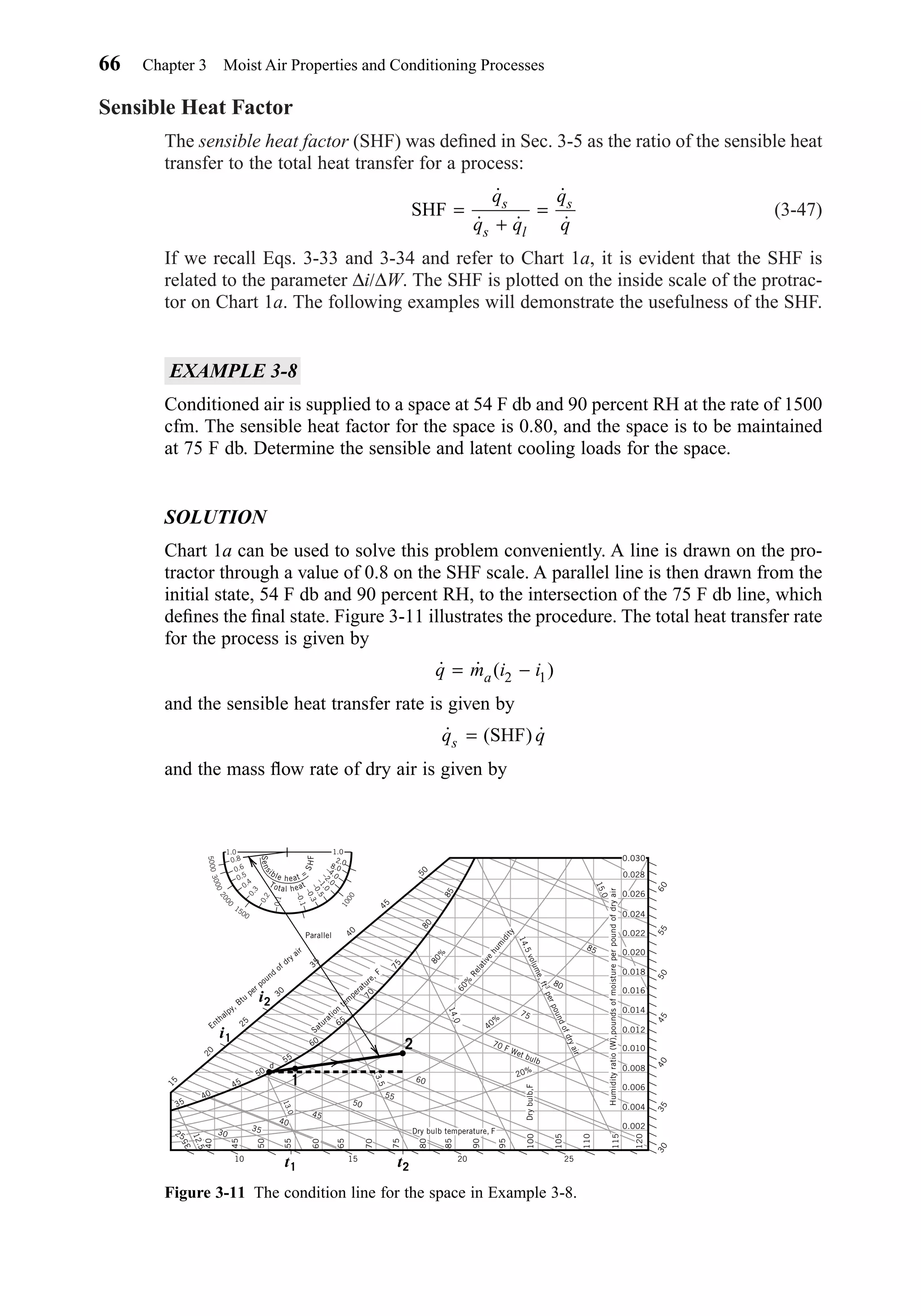
The sensible heat factor (SHF) is defined as qs/q.This parameter is shown on the semi-
circular scale of Fig. 3-5. Note that the SHF can be negative. If we use the standard
sign convention that sensible or latent heat transfer to the system is positive and trans-
fer from the system is negative, the proper sign will result. For example, with the cool-
ing and dehumidifying process above, both sensible and latent heat transfer are away
from the air, qs and ql are both negative, and the SHF is positive. In a situation where
air is being cooled sensibly but a large latent heat gain is present, the SHF will be neg-
ative if the absolute value of ql is greater than qs. The use of this feature of the chart
is shown later.
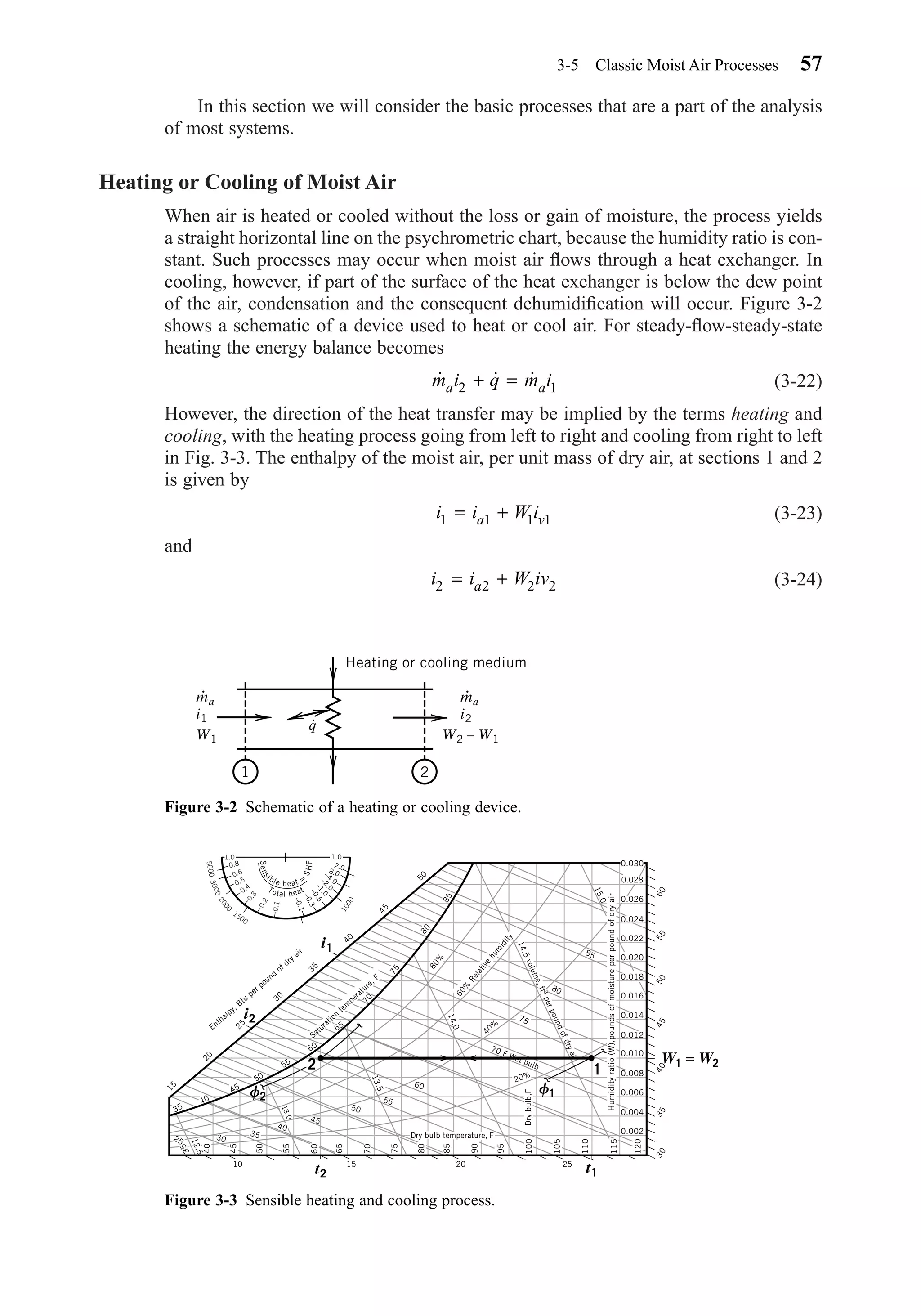
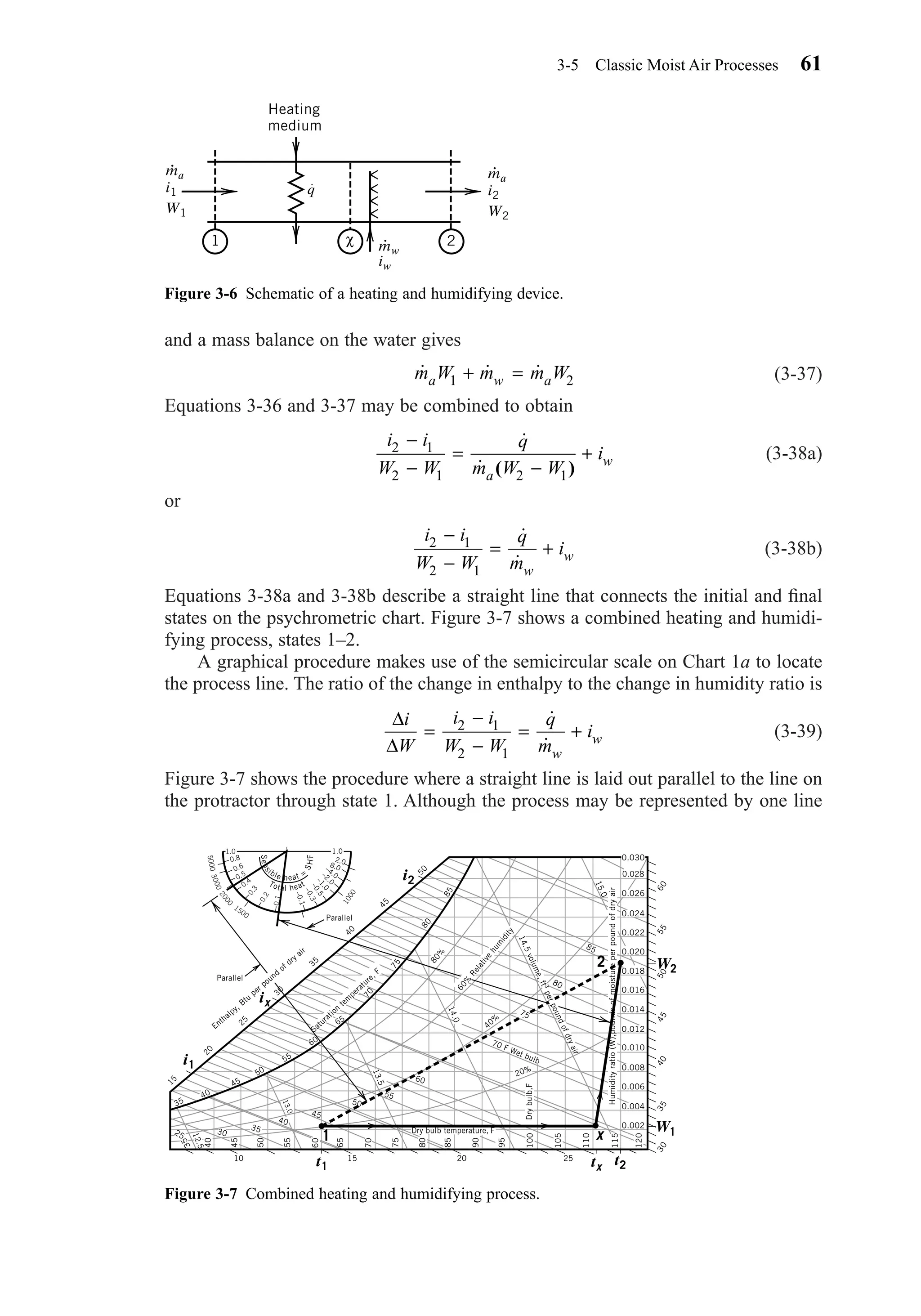
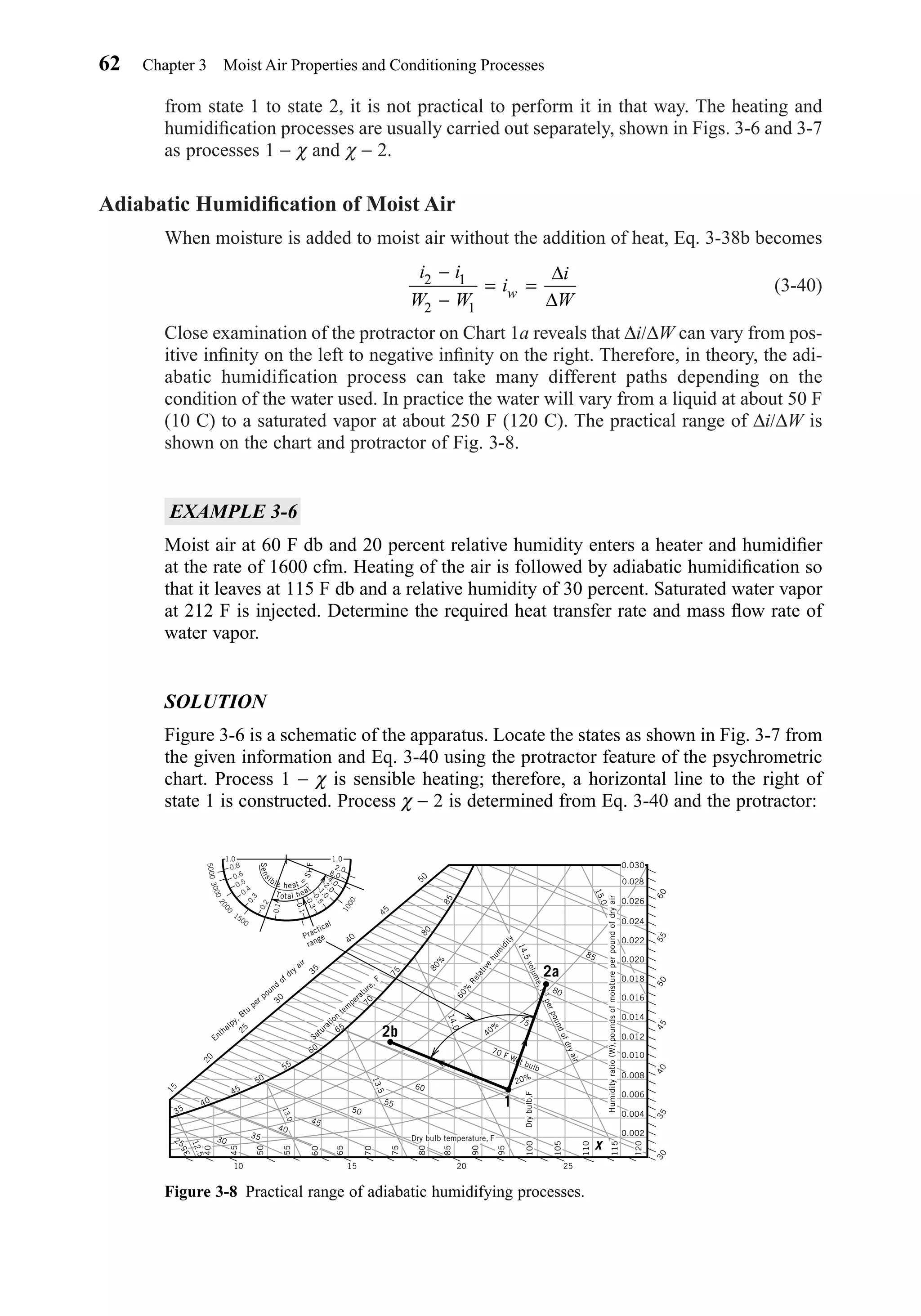
Heating and Humidifying Moist Air
A device to heat and humidify moist air is shown schematically in Fig. 3-6. This
process is generally required to maintain comfort during the cold months of the year.
An energy balance on the device yields
(3-36)˙ ˙ ˙ ˙m i q m i m ia w w a1 2+ + =
˙ ˙ ˙q q qs l= +
˙ ˙ ( )q m i is a= −2 3
˙ ˙ ( )q m i il a= −3 1
˙ ˙ ( )q m W W il a fg= −2 1
˙ ˙ ( )q m c t ts a p= −2 1
˙ ( . . ) ( . . ) .
˙ ( . ) ( . )
q
q
= − − −[ ]
= −[ ]
8646 31 4 22 8 0 0112 0 0082 28 8
8646 8 6 0 084
˙
( )
.
ma = =
2000 60
13 88
8646 lbma/hr
60 Chapter 3 Moist Air Properties and Conditioning Processes
Chapter03.qxd 6/15/04 2:31 PM Page 60](https://image.slidesharecdn.com/fayec-160521192803/75/Faye-c-mc_quiston_-_jerald_d-_parker_-_jeffrey_d-77-2048.jpg)


![acting to maintain the deep body temperature of about 98.6 F (36.9 C) regardless of
the environmental conditions. A normal, healthy person generally feels most com-
fortable when the environment is at conditions where the body can easily maintain a
thermal balance with that environment. ANSI/ASHRAE Standard 55-1992, “Thermal
Environmental Conditions for Human Occupancy” (2), is the basis for much of what
is presented in this section. The standard specifies conditions in which 80 percent or
more of the occupants will find the environment thermally acceptable. Comfort is thus
a subjective matter, depending upon the opinion or judgment of those affected.
The environmental factors that affect a person’s thermal balance and therefore
influence thermal comfort are
• The dry bulb temperature of the surrounding air
• The humidity of the surrounding air
• The relative velocity of the surrounding air
• The temperature of any surfaces that can directly view any part of the body and
thus exchange radiation
In addition the personal variables that influence thermal comfort are activity and
clothing.
Animal and human body temperatures are essentially controlled by a heat balance
that involves metabolism, blood circulation near the surface of the skin, respiration, and
heat and mass transfer from the skin. Metabolism determines the rate at which energy
is converted from chemical to thermal form within the body, and blood circulation con-
trols the rate at which the thermal energy is carried to the surface of the skin. In respi-
ration, air is taken in at ambient conditions and leaves saturated with moisture and very
near the body temperature. Heat transfer from the skin may be by conduction, con-
vection, or radiation. Sweating and the accompanying mass transfer play a very impor-
tant role in the rate at which energy can be carried away from the skin by air.
The energy generated by a person’s metabolism varies considerably with that per-
son’s activity. A unit to express the metabolic rate per unit of body surface area is the
met, defined as the metabolic rate of a sedentary person (seated, quiet): 1 met = 18.4
Btu/(hr-ft2) (58.2 W/m2). Metabolic heat generation rates typical of various activities
are given in the ASHRAE Handbook, Fundamentals Volume (1). The average adult is
assumed to have an effective surface area for heat transfer of 19.6 ft2 (1.82 m2) and
will therefore dissipate approximately 360 Btu/hr (106 W) when functioning in a
quiet, seated manner. A table of total average heat generation for various categories of
persons is given in Chapter 8 and the ASHRAE Handbook (1).
The other personal variable that affects comfort is the type and amount of cloth-
ing that a person is wearing. Clothing insulation is usually described as a single equiv-
alent uniform layer over the whole body. Its insulating value is expressed in terms of
clo units: 1 clo = 0.880 (F-ft2-hr)/Btu [0.155 (m2-C)/W]. Typical insulation values for
clothing ensembles are given in the ASHRAE Handbook (1). A heavy two-piece busi-
ness suit with accessories has an insulation value of about 1 clo, whereas a pair of
shorts has about 0.05 clo.
4-2 ENVIRONMENTAL COMFORT INDICES
In the previous section it was pointed out that, in addition to the personal factors of
clothing and activity that affect comfort, there are four environmental factors: tem-
perature, humidity, air motion, and radiation. The first of these, temperature, is easily
86 Chapter 4 Comfort and Health—Indoor Environmental Quality
Chapter04.qxd 6/15/04 2:31 PM Page 86](https://image.slidesharecdn.com/fayec-160521192803/75/Faye-c-mc_quiston_-_jerald_d-_parker_-_jeffrey_d-103-2048.jpg)

![SOLUTION
The operative temperature depends on the mean radiant temperature, which is given
by Eq. 4-1:
or
Notice that in Eq. 4-1 absolute temperature must be used in the terms involving
the fourth power, but that temperature differences can be expressed in absolute or non-
absolute units.
A good estimate of the operative temperature is
The operative temperature shows the combined effect of the environment’s radiation
and air motion, which for this case gives a value 6 degrees F greater than the sur-
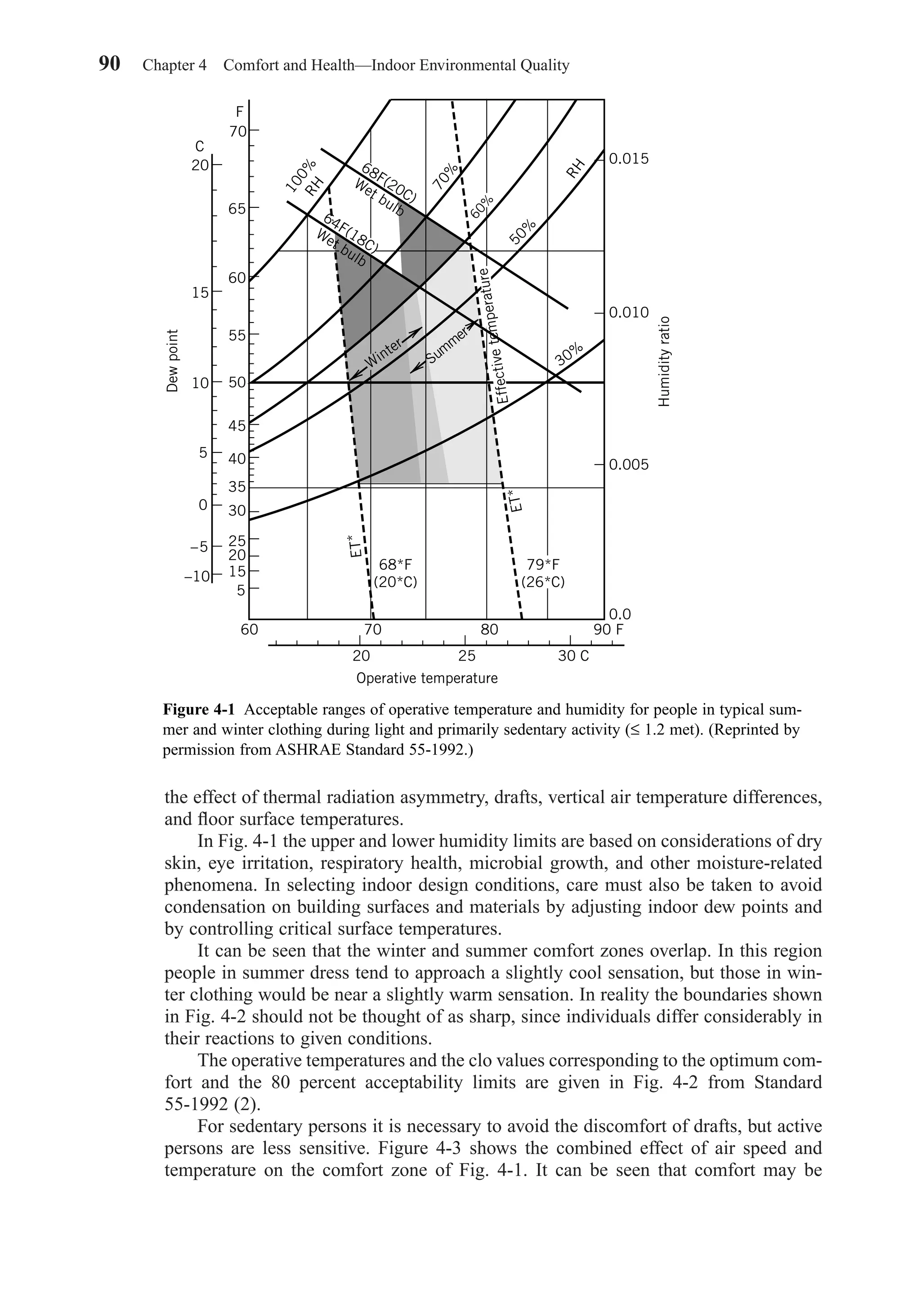
rounding air temperature. Fig. 4-2 shows that this is probably an uncomfortable envi-
ronment. The discomfort is caused by thermal radiation from surrounding warm
surfaces, not from the air temperature. The humidity has not been taken into account,
but at this operative temperature a person would likely be uncomfortable at any level
of humidity.
4-3 COMFORT CONDITIONS
ASHRAE Standard 55-1992 gives the conditions for an acceptable thermal environ-
ment. Most comfort studies involve use of the ASHRAE thermal sensation scale. This
scale relates words describing thermal sensations felt by a participant to a correspon-
ding number. The scale is:
+3 hot
+2 warm
+1 slightly warm
0 neutral
−1 slightly cool
−2 cool
−3 cold
Energy balance equations have been developed that use a predicted mean
vote (PMV) index. The PMV index predicts the mean response of a large group of
people according to the ASHRAE thermal sensation scale. The PMV can be used to
estimate the predicted percent dissatisfied (PPD). ISO Standard 7730 (3) includes com-
puter listings for facilitating the computation of PMV and PPD for a wide range of
parameters.
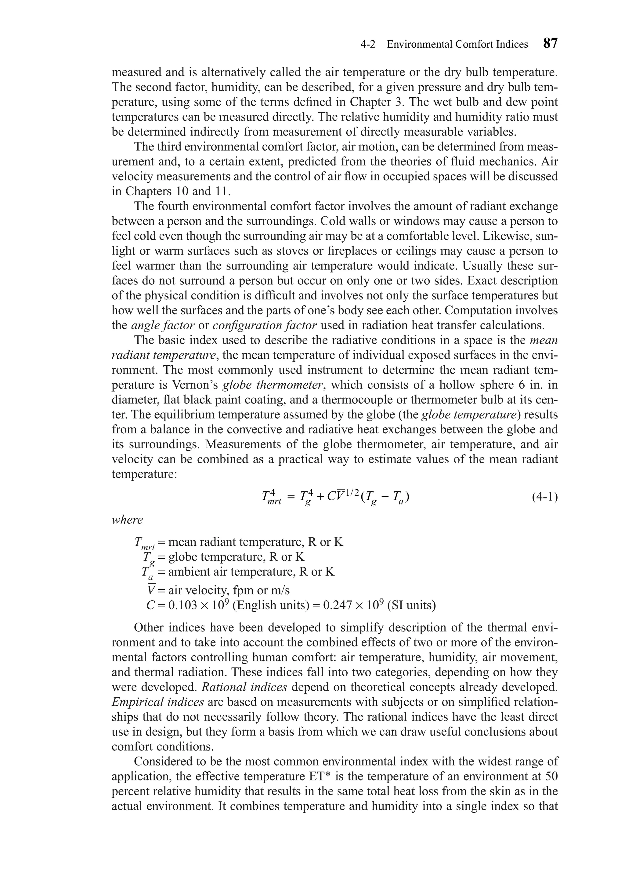
Acceptable ranges of operative temperature and humidity for people in typical
summer and winter clothing during light and primarily sedentary activity (≤ 1.2 met)
are given in Fig. 4-1. The ranges are based on a 10 percent dissatisfaction criterion.
This could be described as general thermal comfort. Local thermal comfort describes
t
t t
to
mrt a
o=
+
=
+
= =
2
86 75
2
80 5 81. , F
T T CV T T
T
mrt g g a
mrt
= + −
= + + × −[ ] = =
[ ( )]
( ) ( . ) ( ) ( )
/ /
/ /
4 1 2 1 4
4 9 1 2 1 4
81 460 0 103 10 30 81 75 546 86R F
T T CV T Tmrt g g a
4 4 1 2= + −/ ( )
4-3 Comfort Conditions 89
Chapter04.qxd 6/15/04 2:31 PM Page 89](https://image.slidesharecdn.com/fayec-160521192803/75/Faye-c-mc_quiston_-_jerald_d-_parker_-_jeffrey_d-106-2048.jpg)


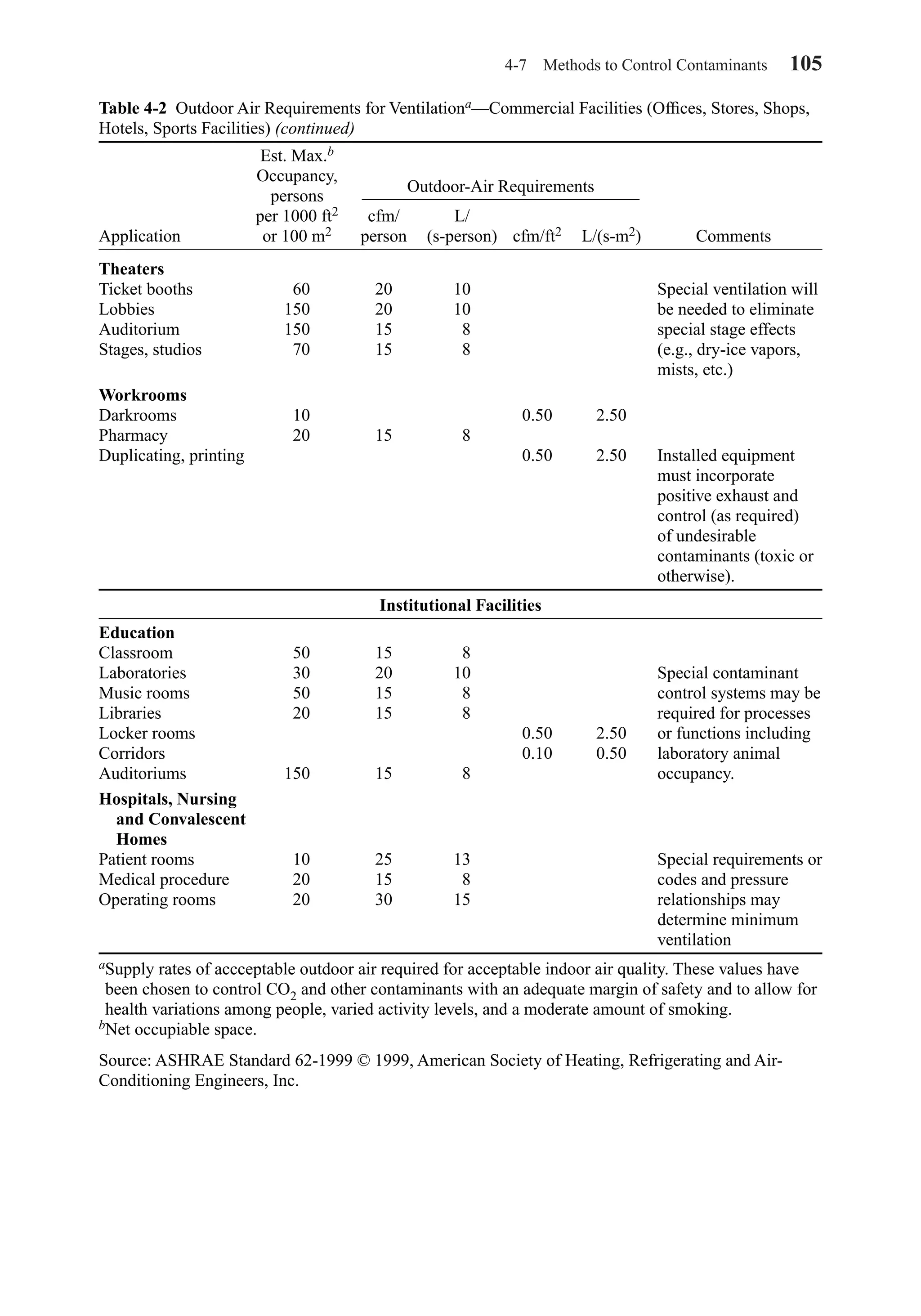
![4-7 Methods to Control Contaminants 103
Table 4-2 Outdoor Air Requirements for Ventilationa—Commercial Facilities (Offices, Stores, Shops,
Hotels, Sports Facilities)
Est. Max.b
Occupancy,
persons
per 1000 ft2 cfm/ L/
Application or 100 m2 person (s-person) cfm/ft2 L/(s-m2) Comments
Food and Beverage
Service
Dining rooms 70 20 10
Cafeteria, fast food 100 20 10
Kitchens (cooking) 20 15 8 Makeup air for hood
exhaust may require
more ventilation air.
The sum of the outdoor
air and transfer air of
acceptable quality
from adjacent
spaces shall be
sufficient to provide
an exhaust rate of
not less than 1.5
cfm/ft2 [7.5L(s-m2)].
Garages, Repair,
Service Stations
Enclosed parking 1.50 7.5 Distribution among
garage people must consider
Auto repair rooms 1.50 7.5 worker location and
concentration of run-
ning engines; stands
where engines are run
must incorporate sys-
tems for positive
engine exhaust with-
drawal. Contaminant
sensors may be used to
control ventilation.
Hotels, Motels,
Resorts,
Dormitories
Cfm/ L/ Independent of room
room (s-room) size.
Bedrooms 30 15
Living rooms 30 15
Baths 35 18 Installed capacity for
intermittent use.
Lobbies 30 15 8
Conference rooms 50 20 10
Assembly rooms 120 15 8
Dormitory 20 15 8 See also food and
sleeping areas beverage services, mer-
chandising, barber and
beauty shops, garages.
continues
Outdoor-Air Requirements
Chapter04.qxd 6/15/04 2:31 PM Page 103](https://image.slidesharecdn.com/fayec-160521192803/75/Faye-c-mc_quiston_-_jerald_d-_parker_-_jeffrey_d-120-2048.jpg)
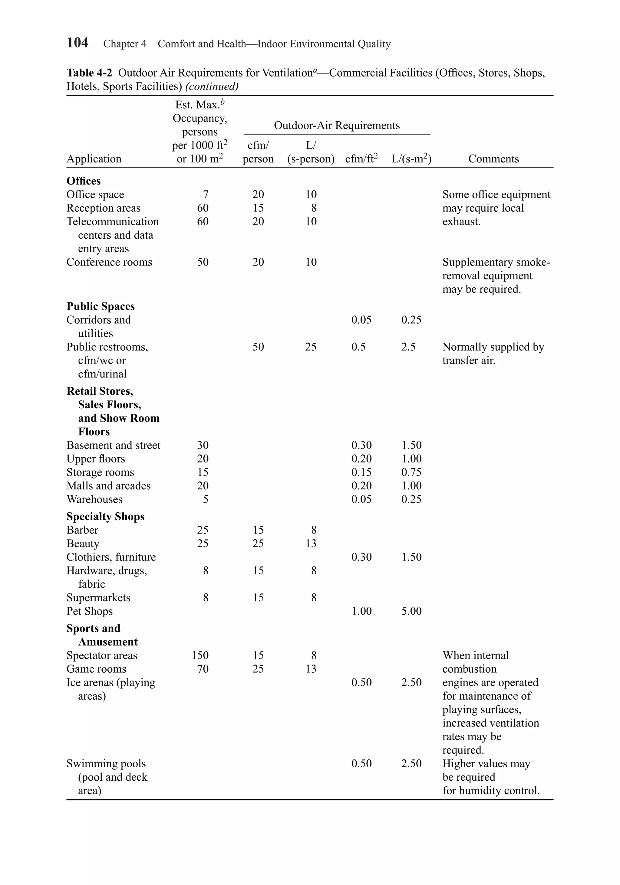
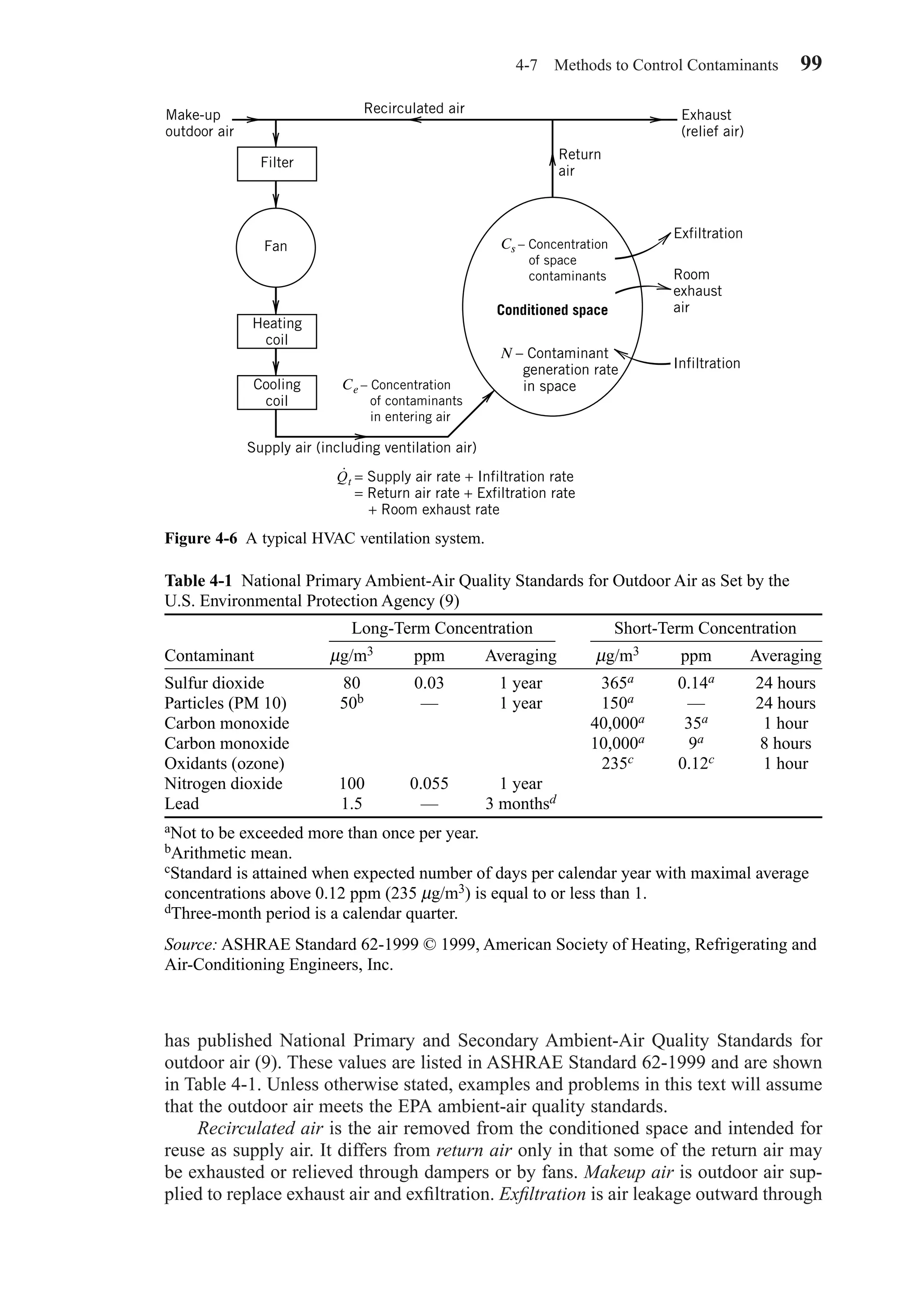
![Standard 62-1999 gives procedures by which the outdoor air can be evaluated for
acceptability. Table 4-1, taken from Standard 62-1999, lists the EPA standards (9) as
the contaminant concentrations allowed in outdoor air. Outdoor-air treatment is pre-
scribed where the technology is available and feasible for any concentrations exceed-
ing the values recommended. Where the best available, demonstrated, and proven
technology does not allow the removal of contaminants, outdoor-air rates may be
reduced during periods of high contaminant levels, but recognizing the need to follow
local regulations.
Indoor air quality is considered acceptable by the Ventilation Rate Procedure if the
required rates of acceptable outdoor air listed in Table 4-2 are provided for the occu-
pied space. Unusual indoor contaminants or sources should be controlled at the source,
or the Indoor Air Quality Procedure, described below, should be followed. Areas within
industrial facilities not covered by Table 4-2 should use threshold limit values of ref-
erence 4. Ventilation guidelines for health care facilities are given in reference 10.
For most of the cases in Table 4-2, outdoor air requirements are assumed to be in
proportion to the number of space occupants and are given in cfm (L/s) per person. In
the rest of the cases the outdoor air requirements are given in cfm/ft2 [L/(s-m2)], and
the contamination is presumed to be primarily due to other factors. Although estimated
maximum occupancy is given where appropriate for design purposes, the anticipated
occupancy should be used. For cases where more than one space is served by a com-
mon supply system, the Ventilation Rate Procedure in Standard 62-1999 provides a
means for calculating the outdoor air requirements for the system. Rooms provided
with exhaust air systems, such as toilet rooms and bathrooms, kitchens, and smoking
lounges, may be furnished with makeup air from adjacent occupiable spaces provided
the quantity of air supplied meets the requirements of Table 4-2.
Except for intermittent or variable occupancy, outdoor air requirements of Table
4-2 must be met under the Ventilation Rate Procedure. Rules for intermittent or vari-
able occupancy are described in Standard 62-1999. If cleaned, recirculated air is to be
used to reduce the outdoor-air rates below these values, then the Indoor Air Quality
Procedure, described below, must be used.
Indoor Air Quality Procedure
The second procedure of Standard 62-1999, the “Indoor Air Quality Procedure,” pro-
vides a direct solution to acceptable IAQ by restricting the concentration of all known
contaminants of concern to some specified acceptable levels. Both quantitative and
subjective evaluations are involved. The quantitative evaluation involves the use of
acceptable indoor contaminant levels from a variety of sources, some of which are tab-
ulated in Standard 62-1999. The subjective evaluation involves the response of impar-
tial observers to odors that might be present in the indoor environment, which can
obviously occur only after the building is complete and operational.
Air cleaning may be used to reduce outdoor air requirements below those given
in Table 4-2 and still maintain the indoor concentration of troublesome contaminants
below the levels needed to provide a safe environment. However, there may be some
contaminants that are not appreciably reduced by the air-cleaning system and that may
be the controlling factor in determining the minimum outdoor air rates required. For
example, the standard specifically requires a maximum of 1000 ppm of CO2, a gas not
commonly controlled by air cleaning. The rationale for this requirement on CO2
was shown in Example 4-2 and is documented in Appendix D of the Standard. The
calculations show that for assumed normal conditions, this maximum concentration
106 Chapter 4 Comfort and Health—Indoor Environmental Quality
Chapter04.qxd 6/15/04 2:31 PM Page 106](https://image.slidesharecdn.com/fayec-160521192803/75/Faye-c-mc_quiston_-_jerald_d-_parker_-_jeffrey_d-123-2048.jpg)


( . )( . )( ) / ( . )
˙ .
=
+ − −
=
125 0 65 20 1 0 7 0 220 0 0283
0 65 0 7 220 0 0283
15 6
3 3 3
3 3 3
µ µ
µ
g cfm g/m m /ft
g m m /f
cfm/person
RQ
N E Q E C C
E E Cr
v o f o s
v f s
˙
˙ ˙ [( ) ]
=
+ − −1
˙
˙ ˙
[ ( ) ]
Q
N E RQ E C
E C E Co
v r f s
v s f o
=
−
− −1
˙
˙ ˙
( )
Q
N E RQ E C
E C Co
v r f s
v s o
=
−
−
Chapter04.qxd 6/15/04 2:31 PM Page 113](https://image.slidesharecdn.com/fayec-160521192803/75/Faye-c-mc_quiston_-_jerald_d-_parker_-_jeffrey_d-130-2048.jpg)
![114 Chapter 4 Comfort and Health—Indoor Environmental Quality
The total rate of supply air to the room Qt = Qo + RQr = 20 + 15.6 = 35.6 cfm/person.
If we assumed that there were about 7 persons per 1000 square feet as typical for an
office (Table 4-2), the air flow to the space would be
This would probably be less than the supply air-flow rate typically required to meet
the cooling load. A less efficient filter might be considered. If the above filter were
used with the same rate of outdoor air but with increased supply and recirculation
rates, the air in the space would be better than the assumed level.
EXAMPLE 4-5
For Example 4-4 assume that the cooling load requires that 1.0 cfm/ft2 be supplied to
the space and determine the recirculation rate per person QrR and the concentration
level of the ETS in the space. Assume that the rate of outdoor air per person and the
filter efficiency remain unchanged.
SOLUTION
Solving Eq. 4-12 for Cs,
The extra recirculation of the air through the filter has reduced the space concentra-
tion level of the tobacco smoke considerably with no use of extra outdoor air.
EXAMPLE 4-6
Assume that the office in Example 4-5 is occupied by 70 persons and that a suitably
efficient filter was the M-15 filter of Fig. 4-8 and Table 4-3. Using this filter, design a
system that has a pressure loss of no more than 0.30 in. wg in the clean condition.
SOLUTION
Table 4-3 gives the application data needed. There are four sizes of M-15 filters to
choose from, and the rated cfm at 0.35 in. wg pressure loss is given for each size. We
must choose an integer number of filter elements. The total supply cfm required for
70 persons is
˙ (Qs = +123 20 70 10 000cfm/person persons cfm)( ) = ,
C
N E Q E C
E Q RQ Es
v o f o
v o r f
=
+ −
+
=
−
+
=
˙ ˙ ( )
( ˙ ˙ )
( )
{ . [ ( )( . )] }( . )
1 125
0 65 20 123 0 7 0 0283 3 3
µ
µ
g min person
cfm/person m /ft
64 g/m3Cs
RQ A Q A Q A t
RQ
r r o
r
˙ / ˙ / ˙ / . ( )( )/ .
˙ ( . )( )
= − = − =
= =
1 0 7 20 1000 0 86
0 86 1000
7
123
2
2 2
cfm/f
cfm/ft ft
persons
cfm/person
˙ /
( .
.Q A = =
35 6 7
1000
0 252
2cfm/person)( persons)
ft
cfm/ft
Chapter04.qxd 6/15/04 2:31 PM Page 114](https://image.slidesharecdn.com/fayec-160521192803/75/Faye-c-mc_quiston_-_jerald_d-_parker_-_jeffrey_d-131-2048.jpg)
![It is desirable for the complete filter unit to have a reasonable geometric shape and
be as compact as possible. Therefore, choose the 24 × 24 × 12 elements for a trial
design. The rated cfm will first be adjusted to obtain a pressure loss of 0.30 in. wg
using Eq. 4-10:
Then the required number of elements is
Since n must be an integer, use 6 elements and the complete filter unit will have
dimensions of 48 × 72 in., a reasonable shape. The filter unit will have a pressure loss
less than the specified 0.30 in. wg. Again, using Eq. 4-10 the actual pressure loss will
be approximately
This is not an undesirable result and can be taken into account in the design of the air
distribution system.
In special applications such as clean rooms, nuclear facilities, and toxic-particulate
applications, very high-efficiency dry filters, HEPA (high-efficiency air particulate air)
filters, and ULPA (ultralow penetration air) filters are the standard to use. These filters
typically have relatively high resistance to air flow.
REFERENCES
1. ASHRAE Handbook, Fundamentals Volume, American Society of Heating, Refrigerating and Air-Con-
ditioning Engineers, Inc., Atlanta, GA, 2001.
2. ANSI/ASHRAE Standard 55-1992, “Thermal Environmental Conditions for Human Occupancy,”
American Society of Heating, Refrigerating and Air-Conditioning Engineers, Inc., Atlanta, GA, 1992.
3. ISO Standard 7730, “Moderate Thermal Environments—Determination of the PMV and PPD Indices
and Specifications of the Conditions for Thermal Comfort,” ISO, 1984.
4. ANSI/ASHRAE Standard 113-1990, “Method of Testing for Room Air Diffusion,” American Society
of Heating, Refrigerating and Air-Conditioning Engineers, Inc., Atlanta, GA, 1990.
5. ASHRAE Thermal Comfort Tool CD, ASHRAE Research Project 781, Code 94030, American Soci-
ety of Heating, Refrigerating and Air-Conditioning Engineers, Inc., Atlanta, GA, 1997.
6. ANSI/ASHRAE Standard 62-1999, “Ventilation for Acceptable Indoor Air Quality,” American Soci-
ety of Heating, Refrigerating and Air-Conditioning Engineers, Inc., Atlanta, GA, 1999.
7. Jan Sundell, “What We Know and Don’t Know About Sick Building Syndrome,” ASHRAE Journal,
pp. 51–57, June 1996.
8. Lew Harriman, Geoff Brundrett, and Reinhold Kittler, Humidity Control Design Guide for Commer-
cial and Institutional Buildings, American Society of Heating, Refrigerating and Air-Conditioning
Engineers, Inc., Atlanta, GA, 2001.
9. EPA, National Primary and Secondary Ambient-Air Quality Standards, Code of Federal Regulations,
Title 40, Part 50 (40 CFR 50) as amended July 1, 1987, U.S. Environmental Protection Agency.
10. AIA, Guidelines for Design and Construction of Hospital and Health Care Facilities, The American
Institute of Architects Press, Washington, DC, 2001.
11. William J. Coad, “Indoor Air Quality: A Design Parameter,” ASHRAE Journal, pp. 39–47, June 1996.
12. ASHRAE Handbook, HVAC Applications Volume, American Society of Heating, Refrigerating and
Air-Conditioning Engineers, Inc., Atlanta, GA, 2002.
13. ASHRAE Handbook, HVAC Systems and Equipment Volume, American Society of Heating, Refriger-
ating and Air-Conditioning Engineers, Inc., Atlanta, GA, 2000.
14. ANSI/ASHRAE Standard 52.1-1992, “Gravimetric and Dust-Spot Procedures for Testing Air Clean-
ing Devices Used in General Ventilation for Removing Particulate Matter,” American Society of Heat-
ing, Refrigerating and Air-Conditioning Engineers, Inc., Atlanta, GA, 1992.
∆ ∆p p Q Qr r= = =[ ˙/ ˙ ] . [( , / )/ ] .2 20 35 10 000 6 2000 0 24 in.wg
n Q Qs n= = =˙ / ˙ , / .10 000 1852 5 40 elements
˙ ˙ ( / ) ( . / . )/ /Q Q p pn r n r= = =∆ ∆ /1 2 1 22000 0 3 0 35 1852 cfm element
References 115
Chapter04.qxd 6/15/04 2:31 PM Page 115](https://image.slidesharecdn.com/fayec-160521192803/75/Faye-c-mc_quiston_-_jerald_d-_parker_-_jeffrey_d-132-2048.jpg)


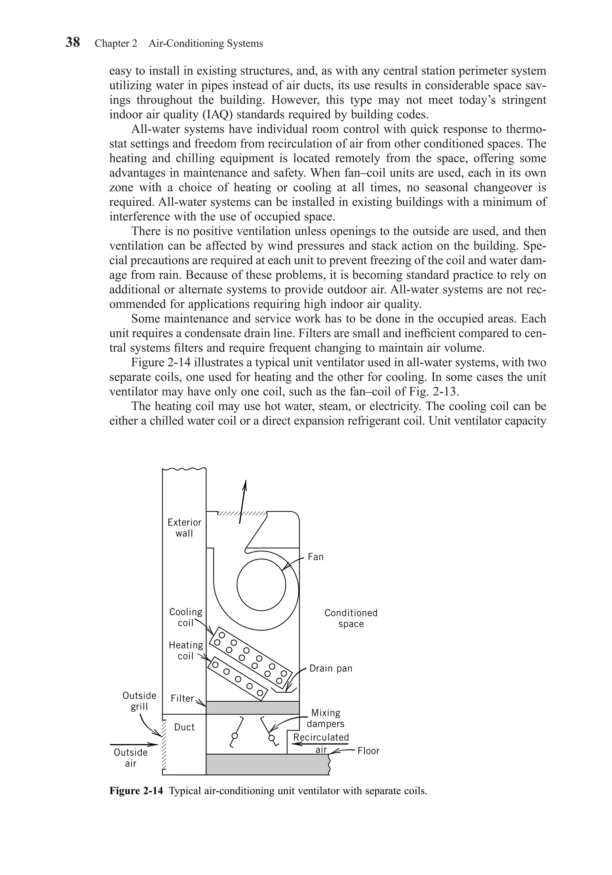
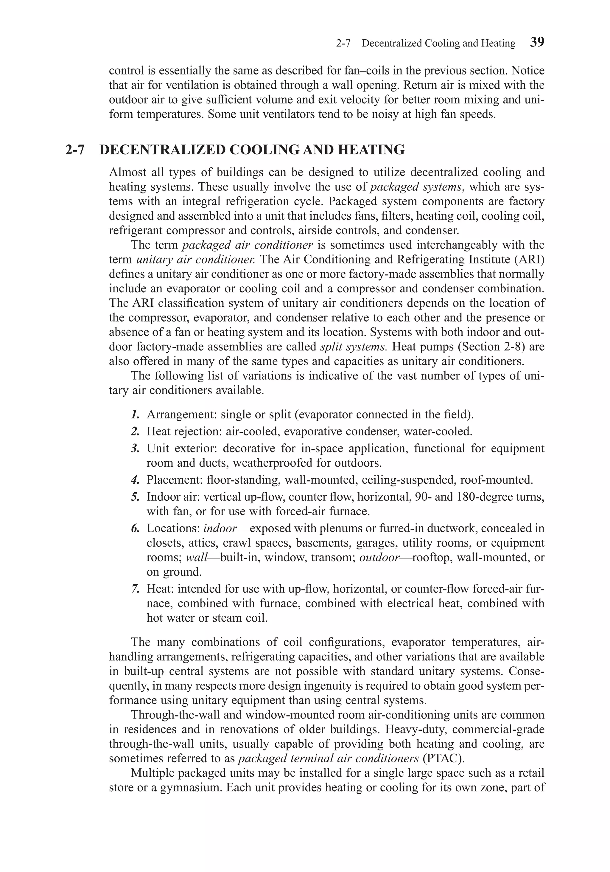
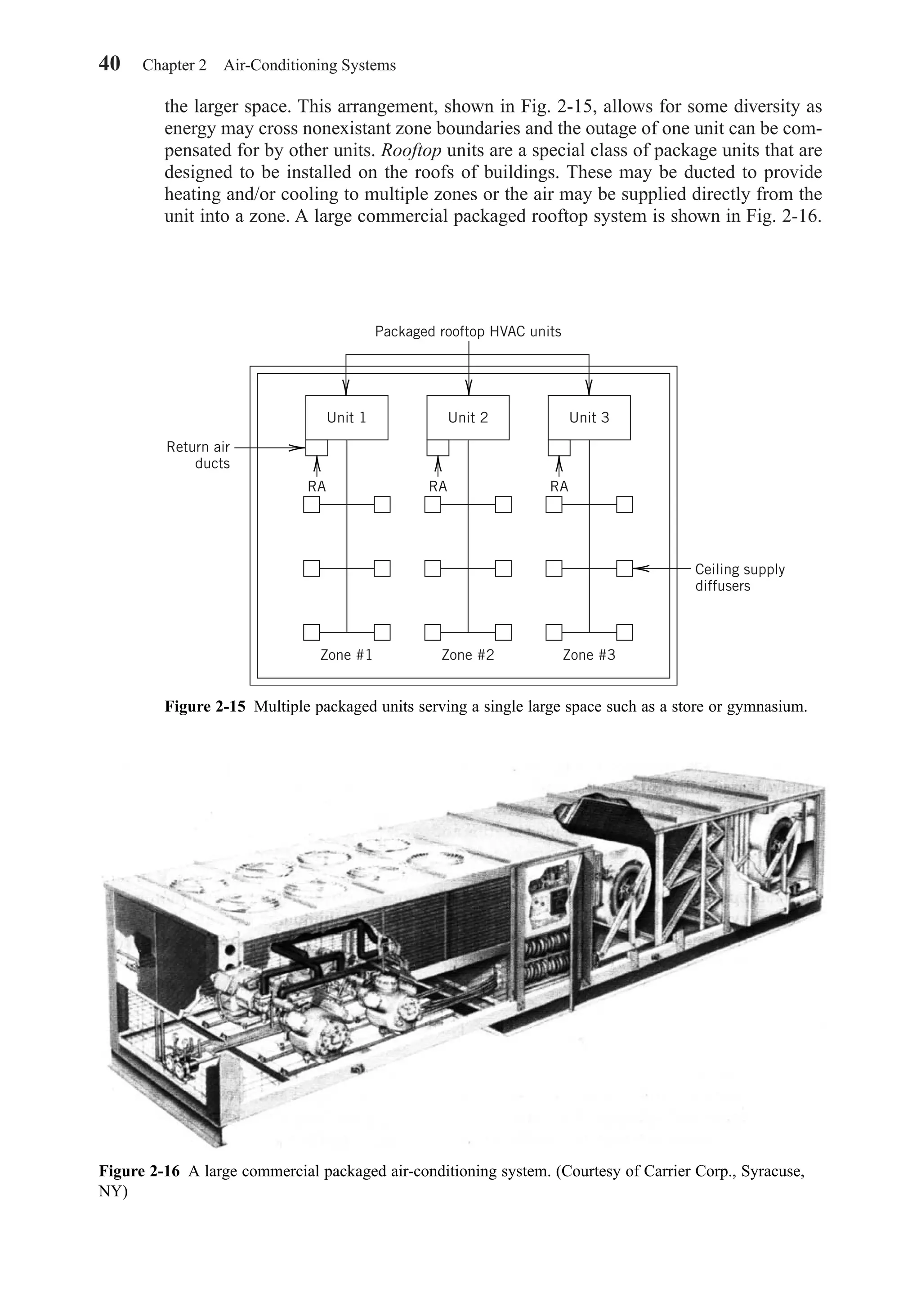
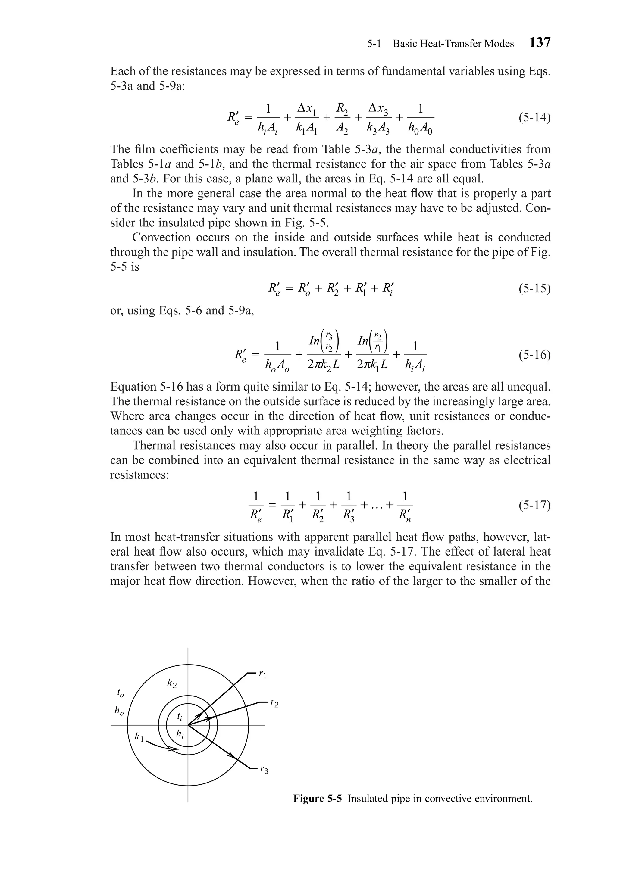
![The film coefficient h is sometimes called the unit surface conductance or alterna-
tively the convective heat transfer coefficient. Equation 5-8a may also be expressed in
terms of thermal resistance:
(5-8b)
where
(5-9a)
so that
(5-9b)
The thermal resistance given by Eq. 5-9a may be summed with the thermal resistances
arising from pure conduction given by Eqs. 5-3a or 5-6.
The film coefficient h appearing in Eqs. 5-8a and 5-9a depends on the fluid, the
fluid velocity, the flow channel or wall shape or orientation, and the degree of devel-
opment of the flow field (that is, the distance from the entrance or wall edge and from
the start of heating). Many correlations exist for predicting the film coefficient under
various conditions. Correlations for forced convection are given in Chapter 3 of the
ASHRAE Handbook (1) and in textbooks on heat transfer.
In convection the mechanism that is causing the fluid motion to occur is impor-
tant. When the bulk of the fluid is moving relative to the heat transfer surface, the
mechanism is called forced convection, because such motion is usually caused by a
blower, fan, or pump that is forcing the flow. In forced convection buoyancy forces are
negligible. In free convection, on the other hand, the motion of the fluid is due entirely
to buoyancy forces, usually confined to a layer near the heated or cooled surface. The
surrounding bulk of the fluid is stationary and exerts a viscous drag on the layer of
moving fluid. As a result inertia forces in free convection are usually small. Free con-
vection is often referred to as natural convection.
Natural or free convection is an important part of HVAC applications. However,
the predicted film coefficients have a greater uncertainty than those of forced convec-
tion. Various empirical relations for natural convection film coefficients can be found
in the ASHRAE Handbook (1) and in heat-transfer textbooks.
Most building structures have forced convection due to wind along outer walls or
roofs, and natural convection occurs inside narrow air spaces and on the inner walls.
There is considerable variation in surface conditions, and both the direction and magni-
tude of the air motion (wind) on outdoor surfaces are very unpredictable. The film coef-
ficient for these situations usually ranges from about 1.0 Btu/(hr-ft2-F) [6 W/(m2-C)] for
free convection up to about 6 Btu/(hr-ft2-F) [35 W/(m2-C)] for forced convection with
an air velocity of about 15 miles per hour (20 ft/sec, 6 m/s). With free convection film
coefficients are low, and the amount of heat transferred by thermal radiation may be
equal to or larger than that transferred by convection.
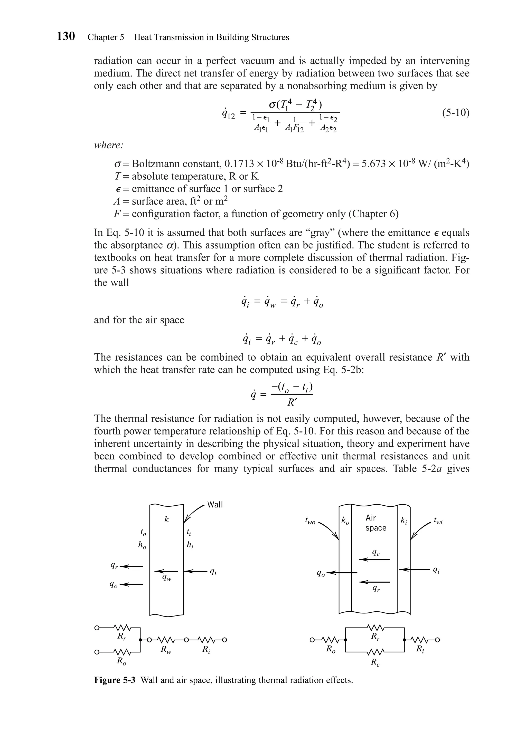
Thermal radiation is the transfer of thermal energy by electromagnetic waves,
an entirely different phenomenon from conduction and convection. In fact, thermal
R
h C
= =
1 1
*
( )/hr-ft -F Btu or (m -C)/W2 2
′ =R
hA
1
(hr-ft)/Btu or C/W
˙q
t t
R
w
=
−
′
5-1 Basic Heat-Transfer Modes 129
*Note that the symbol for conductance is C, in contrast to the symbol for the temperature in Celsius
degrees, C.
Chapter05.qxd 6/15/04 2:31 PM Page 129](https://image.slidesharecdn.com/fayec-160521192803/75/Faye-c-mc_quiston_-_jerald_d-_parker_-_jeffrey_d-146-2048.jpg)
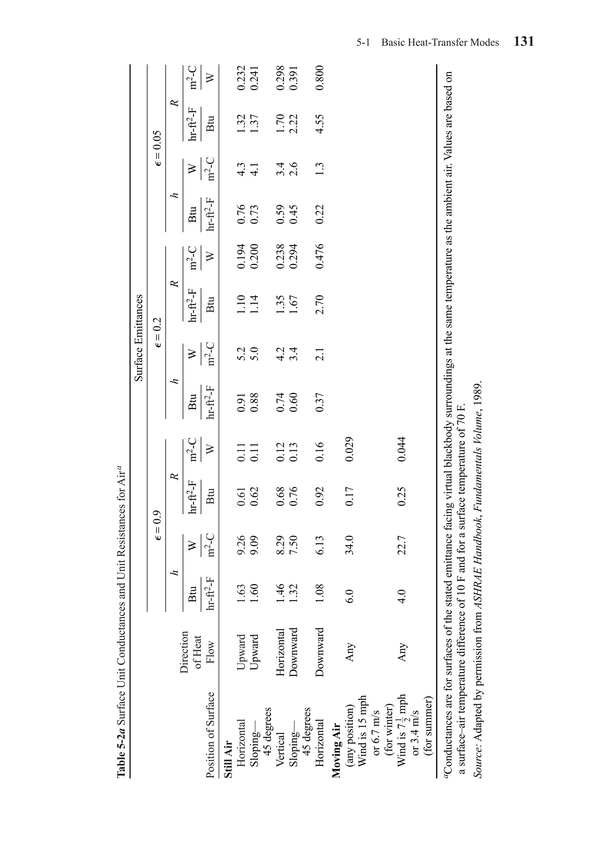
![132 Chapter 5 Heat Transmission in Building Structures
surface film coefficients and unit thermal resistances as a function of wall position,
direction of heat flow, air velocity, and surface emittance for exposed surfaces such as
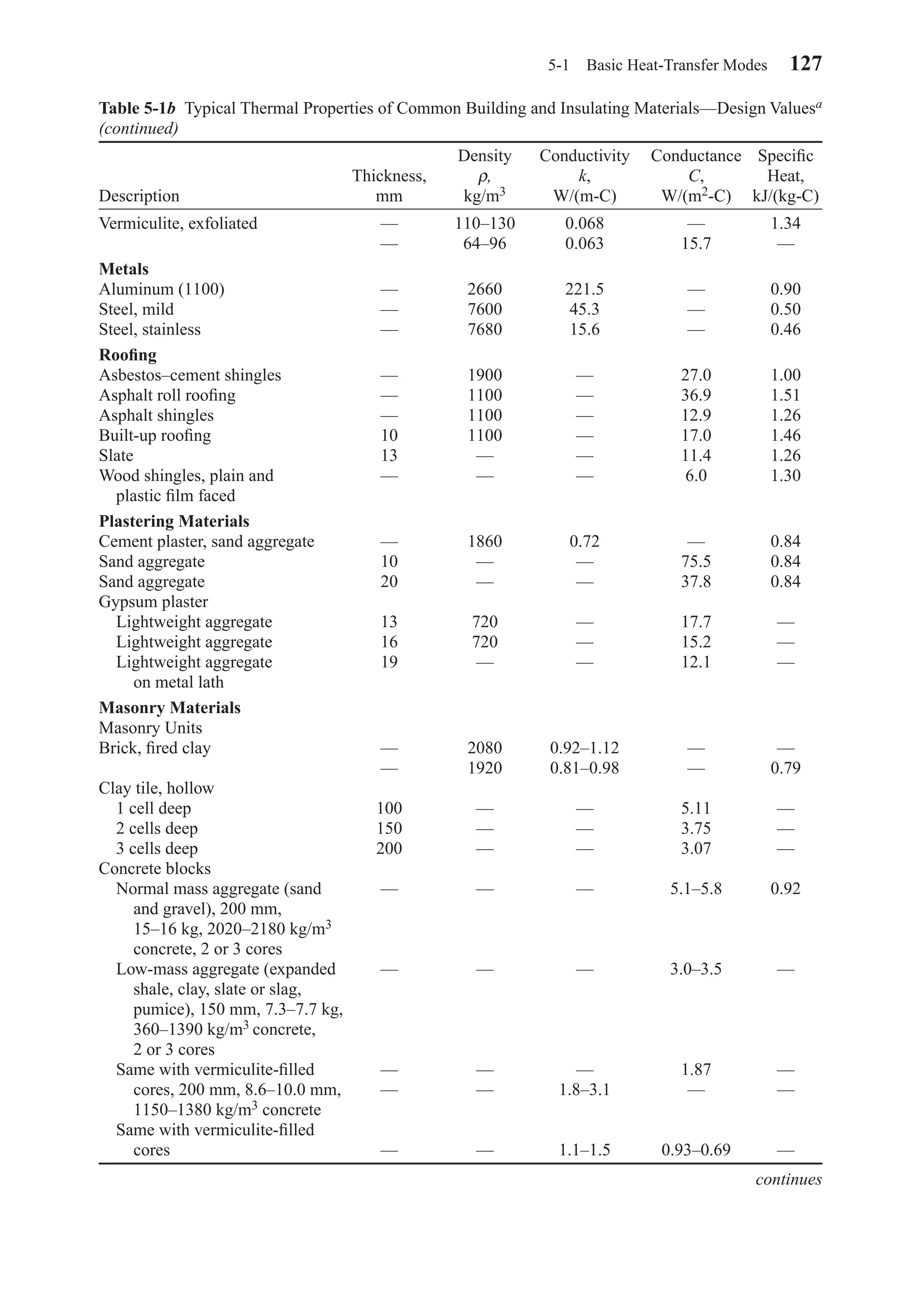
outside walls. Table 5-2b gives representative values of emittance ⑀ for some building
and insulating materials. For example, a vertical brick wall in still air has an emittance
⑀ of about 0.9. In still air the average film coefficient, from Table 5-2a, is about 1.46
Btu/(hr-ft2-F) or 8.29 W/(m2-C), and the unit thermal resistance is 0.68 (hr-ft2-F)/
Btu or 0.12 (m2-C)/W.
If the surface were highly reflective, ⑀ = 0.05, the film coefficient would be 0.59
Btu/(hr-ft2-F) [3.4 W/(m2-C)] and the unit thermal resistance would be 1.7 (hr-ft2-F)/
Btu [0.298 (m2-C)/W]. It is evident that thermal radiation is a large factor when nat-
ural convection occurs. If the air velocity were to increase to 15 mph (about 7 m/s),
the average film coefficient would increase to about 6 Btu/(hr-ft2-F) [34 W/(m2-C)].
With higher air velocities the relative effect of radiation diminishes. Radiation appears
to be very important in the heat gains through ceiling spaces.
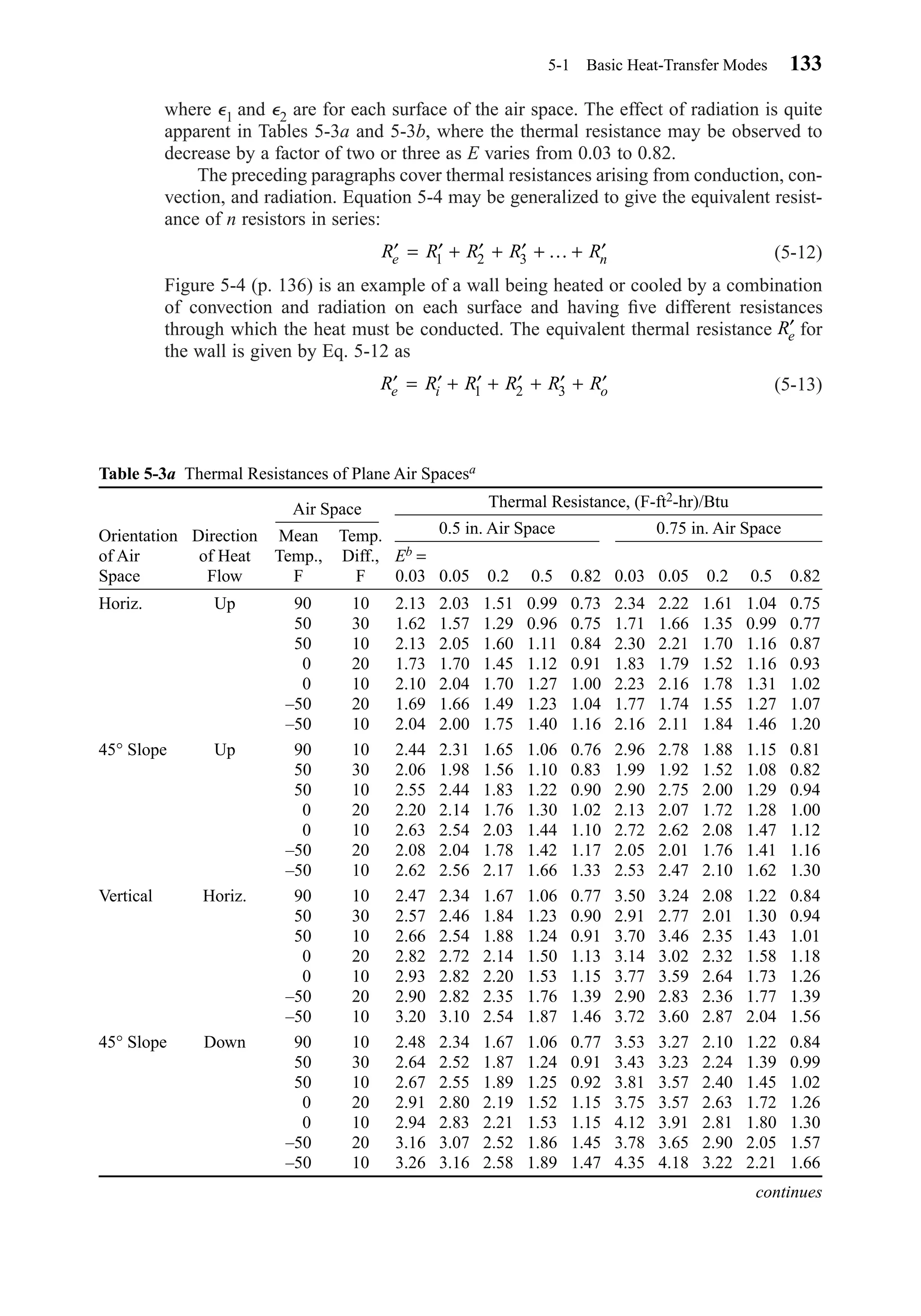
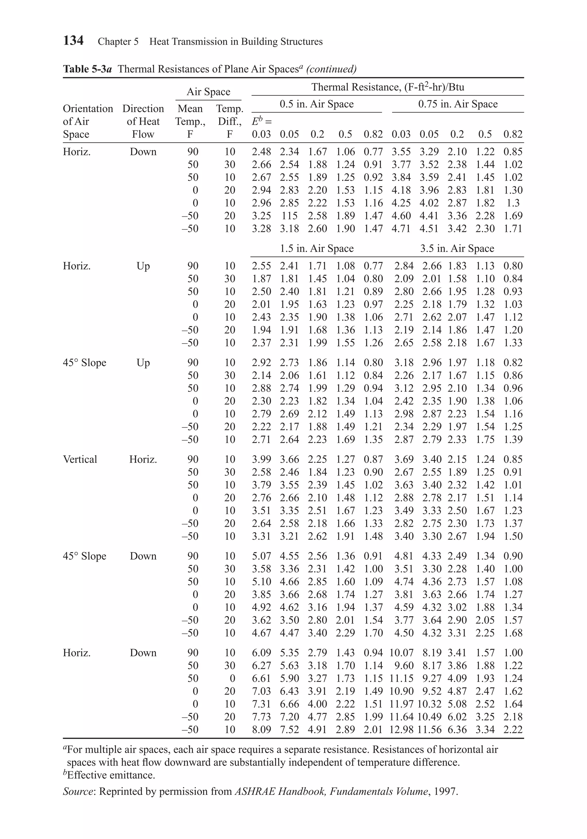
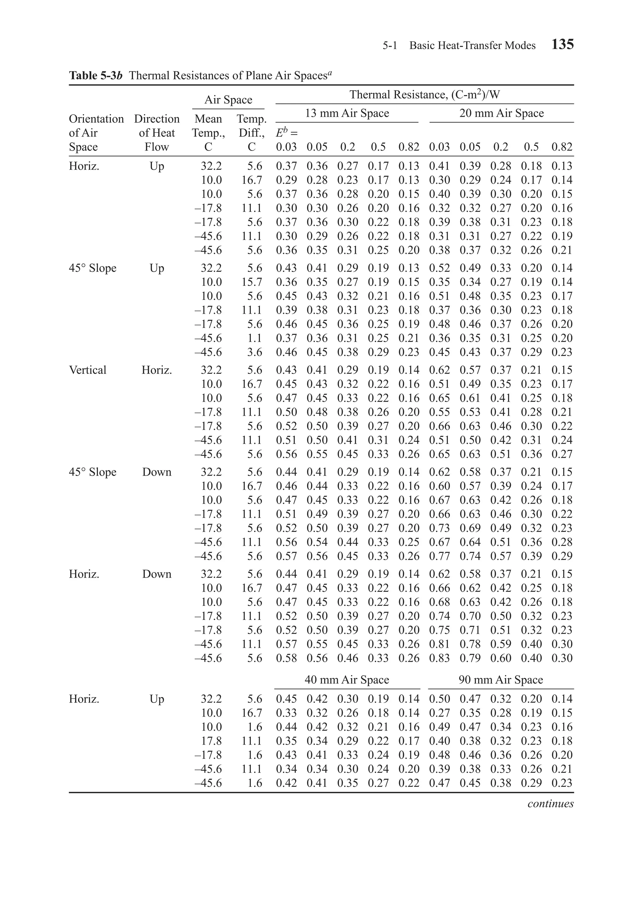
Tables 5-3a and 5-3b give conductances and resistances for air spaces as a func-
tion of orientation, direction of heat flow, air temperature, and the effective emittance
of the space. The effective emittance E is given by
(5-11)
1 1 1
1
1 2E
− + −
⑀ ⑀
⑀
Table 5-2b Reflectance and Emittance of Various Surfaces and Effective Emittances of Air Spacea
With One
Average Surface Having With Both
Emittance Emittance ⑀ and Surfaces
Surface ⑀ Other 0.90 of Emittance ⑀
Aluminum foil, 0.05 0.05 0.03
bright
Aluminum foil, with 0.30b 0.29 —
condensate clearly
visible (> 0.7 gr/ft2)
Aluminum foil, with 0.7b 0.65 —
condensate clearly
visible (> 2.9 gr/ft2)
Regular glass 0.84 0.77 0.72
Aluminum sheet 0.12 0.12 0.06
Aluminum-coated 0.20 0.20 0.11
paper, polished
Steel, galvanized, 0.25 0.24 0.15
bright
Aluminum paint 0.50 0.47 0.35
Building materials— 0.90 0.82 0.82
wood, paper, masonry,
nonmetallic paints
aThese values apply in the 4–40 µm range of the electromagnetic spectrum.
bValues are based on data presented by Bassett and Trethowen (1984).
Source: ASHRAE Handbook–Fundamentals. © American Society of Heating, Refrigerating and Air-
Conditioning Engineers, Inc., 2001.
Effective Emittance E of Air Space
Chapter05.qxd 6/15/04 2:31 PM Page 132](https://image.slidesharecdn.com/fayec-160521192803/75/Faye-c-mc_quiston_-_jerald_d-_parker_-_jeffrey_d-149-2048.jpg)
![so that
Then using Eq. 5-18 we get
EXAMPLE 5-2
Compute the overall average coefficient for the roof–ceiling combination shown in
Table 5-4b with 3.5 in. of mineral fiber batt insulation (R-15) in the ceiling space
rather than the rigid roof deck insulation.
SOLUTION
The total unit resistance of the ceiling–floor combination in Table 5-4b, construction
1, with no insulation is 4.73 (hr-ft2-F)/Btu. Assume an air space greater than 3.5 in.
Total resistance without insulation 4.73
Add mineral fiber insulation, 3.5 in. 15.00
Total R [(hr-ft2-F)/Btu] 19.73
Total U [Btu/(ft2-hr-F)] 0.05
The data given in Tables 5-4a and 5-4b and Examples 5-1 and 5-2 are based on
1. Steady-state heat transfer
2. Ideal construction methods
3. Surrounding surfaces at ambient air temperature
4. Variation of thermal conductivity with temperature negligible
Some caution should be exercised in applying calculated overall heat transfer coeffi-
cients such as those of Tables 5-4a and 5-4b, because the effects of poor workman-
ship and materials are not included. Although a safety factor is not usually applied, a
moderate increase in U may be justified in some cases.
The overall heat-transfer coefficients obtained for walls and roofs should always
be adjusted for thermal bridging, as shown in Tables 5-4a and 5-4b, using Eq. 5-18.
This adjustment will normally be 5 to 15 percent of the unadjusted coefficient.
The coefficients of Tables 5-4a and 5-4b have all been computed for a 15 mph
wind velocity on outside surfaces and should be adjusted for other velocities. The data
of Table 5-2a may be used for this purpose.
The following example illustrates the calculation of an overall heat-transfer coef-
ficient for an unvented roof–ceiling system.
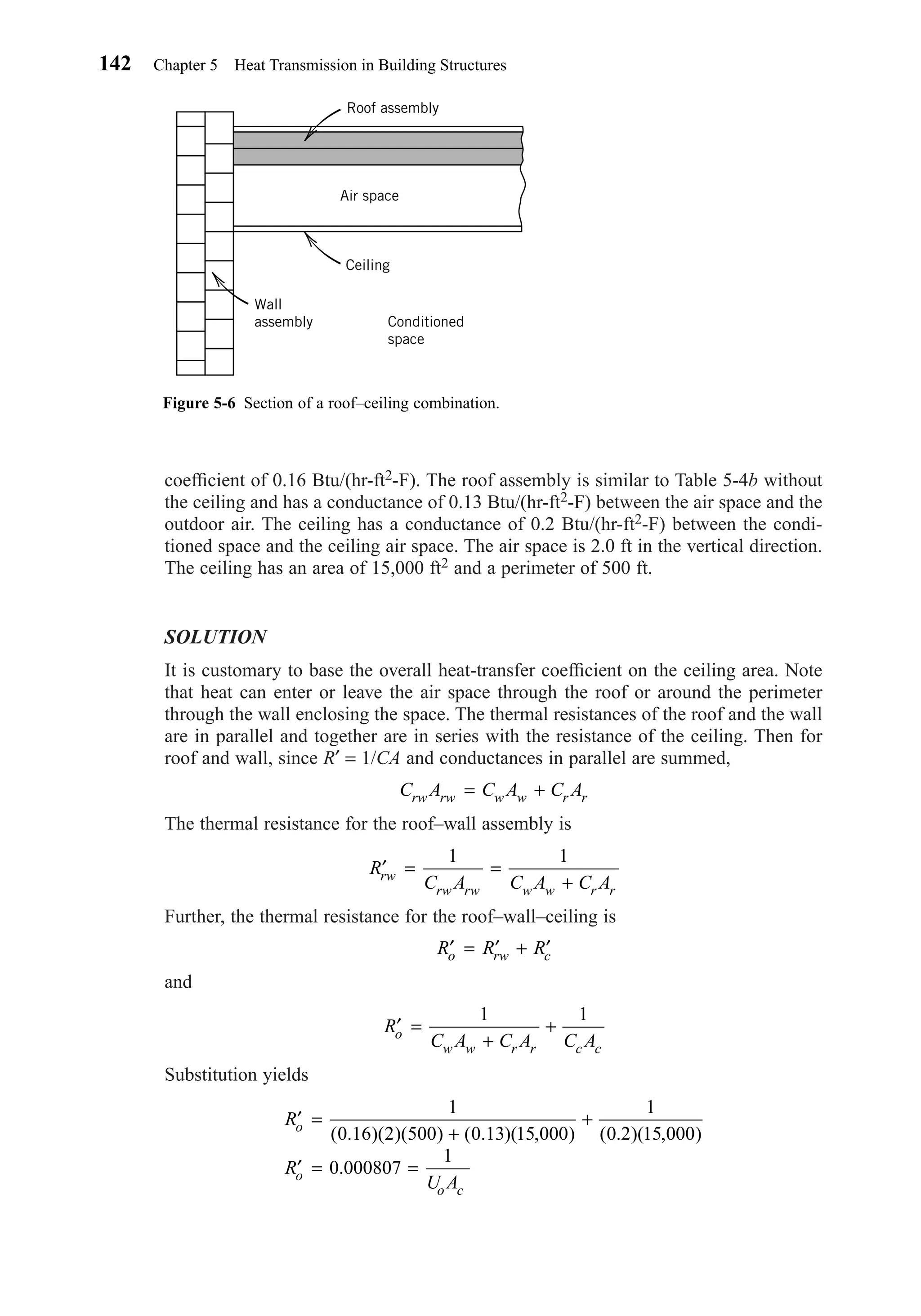
EXAMPLE 5-3
Compute the overall heat-transfer coefficient for the roof–ceiling combination shown
in Fig. 5-6. The wall assembly is similar to Table 5-4a with an overall heat-transfer
Uc =
+
=
( . )( . ) ( . )( . )
.
0 055 14 5 0 140 1 5
16
0 063Btu/(hr-ft -F)2
Uf = 0 140. Btu/(hr-ft -F)2
5-2 Tabulated Overall Heat-Transfer Coefficients 141
Chapter05.qxd 6/15/04 2:31 PM Page 141](https://image.slidesharecdn.com/fayec-160521192803/75/Faye-c-mc_quiston_-_jerald_d-_parker_-_jeffrey_d-158-2048.jpg)
![146 Chapter 5 Heat Transmission in Building Structures
Table 5-6 Representative Fenestration Frame U-Factors, Btu/(hr-ft2-F) or W/(m2-K)
(Vertical Installation)
Type of
Framed Material Spacer Singleb Doublec Tripled Singleb Doublec Tripled
Aluminum without All 2.38 2.27 2.20 1.92 1.80 1.74
thermal break (13.51) (12.89) (12.49) (10.90) (10.22) (9.88)
Aluminum with Metal 1.20 0.92 0.83 1.32 1.13 1.11
thermal breaka (6.81) (5.22) (4.71) (7.49) (6.42) (6.30)
Insulated n/a 0.88 0.77 n/a 1.04 1.02
(n/a) (5.00) (4.37) (n/a) (5.91) (5.79)
Aluminum-clad wood/ Metal 0.60 0.58 0.51 0.55 0.51 0.48
reinforced vinyl (3.41) (3.29) (2.90) (3.12) (2.90) (2.73)
Insulated n/a 0.55 0.48 n/a 0.48 0.44
(n/a) (3.12) (2.73) (n/a) (2.73) (2.50)
Wood vinyl Metal 0.55 0.51 0.48 0.55 0.48 0.42
(3.12) (2.90) (2.73) (3.12) (2.73) (2.38)
Insulated n/a 0.49 0.40 n/a 0.42 0.35
(n/a) (2.78) (2.27) (n/a) (2.38) (1.99)
Insulated fiberglass/ Metal 0.37 0.33 0.32 0.37 0.33 0.32
vinyl (2.10) (1.87) (1.82) (2.10) (1.87) (1.82)
Insulated n/a 0.32 0.26 n/a 0.32 0.26
(n/a) (1.82) (1.48) (n/a) (1.82) (1.48)
Note: This table should only be used as an estimating tool for the early phases of design.
aDepends strongly on width of thermal break. Value given is for in. (9.5 mm) (nominal).
bSingle glazing corresponds to individual glazing unit thickness of in. (3 mm) (nominal).
cDouble glazing corresponds to individual glazing unit thickness of in. (19 mm) (nominal).
dTriple glazing corresponds to individual glazing unit thickness of in. (34.9 mm) (nominal).
Source: ASHRAE Handbook, Fundamentals Volume. © American Society of Heating, Refrigerating and
Air-Conditioning Engineers, Inc., 2001.
1 3
8
3
4
1
8
3
8
Operable
Product Type/Number of Glazing Layers
Fixed
Table 5-7 Glazing U-Factor for Various Wind Speeds
U-Factor, Btu/(hr-ft2-F) [W/(m2-C)]
Wind Speed 15 (24) 7.5 (12) 0 mph (km/h)
0.10 (0.5) 0.10 (0.46) 0.10 (0.42)
0.20 (1.0) 0.20 (0.92) 0.19 (0.85)
0.30 (1.5) 0.29 (1.33) 0.28 (1.27)
0.40 (2.0) 0.38 (1.74) 0.37 (1.69)
0.50 (2.5) 0.47 (2.15) 0.45 (2.12)
0.60 (3.0) 0.56 (2.56) 0.53 (2.54)
0.70 (3.5) 0.65 (2.98) 0.61 (2.96)
0.80 (4.0) 0.74 (3.39) 0.69 (3.38)
0.90 (4.5) 0.83 (3.80) 0.78 (3.81)
1.0 (5.0) 0.92 (4.21) 0.86 (4.23)
1.1 (5.5) 1.01 (4.62) 0.94 (4.65)
1.2 (6.0) 1.10 (5.03) 1.02 (5.08)
1.3 (6.5) 1.19 (5.95) 1.10 (5.50)
Source: Reprinted with permission from ASHRAE
Handbook, Fundamentals Volume, 1997.
Chapter05.qxd 6/15/04 2:31 PM Page 146](https://image.slidesharecdn.com/fayec-160521192803/75/Faye-c-mc_quiston_-_jerald_d-_parker_-_jeffrey_d-163-2048.jpg)
![5-2 Tabulated Overall Heat-Transfer Coefficients 147
Table 5-8 Transmission Coefficients U for Wood and Steel Doors
No Metal
Nominal Door Storm Storm
Thickness in. (mm) Description Door Door1a
Wood Doorsb,c Btu/(hr-ft2-F) [W/(m2-c)]
(35) Panel door with in. panelsd 0.57 (3.24) 0.37 (2.10)
(35) Hollow core flush door 0.47 (2.67) 0.32 (1.82)
(35) Solid core flush door 0.39 (2.21) 0.28 (1.59)
(45) Panel door with in. panelsd 0.54 (3.07) 0.36 (2.04)
(45) Hollow core flush door 0.46 (2.61) 0.32 (1.82)
(45) Panel door with in. panelsd 0.39 (2.21) 0.28 (1.59)
(45) Solid core flush door 0.40 (2.27) 0.26 (1.48)
(57) Solid core flush door 0.27 (1.53) 0.21 (1.19)
Steel Doorsc
(45) Fiberglass or mineral wool core with steel 0.60 (3.41) —
stiffeners, no thermal breake
(45) Paper honeycomb core without thermal breake 0.56 (3.18) —
(45) Solid urethane foam core without thermal breakb 0.40 (2.27) —
(45) Solid fire-rated mineral fiberboard core without 0.38 (2.16) —
thermal breake
(45) Polystyrene core without thermal break 0.35 (1.99) —
(18-gage commercial steel)e
(45) Polyurethane core without thermal break 0.29 (1.65) —
(18-gage commercial steel)e
(45) Polyurethane core without thermal break 0.29 (1.65) —
(24-gage commercial steel)e
(45) Polyurethane core with thermal break and wood 0.20 (1.14) —
perimeter (24-gage residential steel)e
(45) Solid urethane foam core with thermal breakb 0.20 (1.14) 0.16 (0.91)
Note: All U-factors are for exterior door with no glazing, except for the storm doors that are in addition
to the main exterior door. Any glazing area in exterior doors should be included with the appropriate
glass type and analyzed. Interpolation and moderate extrapolation are permitted for door thicknesses
other than those specified.
aValues for metal storm door are for any percent glass area.
bValues are based on a nominal 32 × 80 in. door size with no glazing.
cOutside air conditions: 15 mph wind speed, 0 F air temperature; inside air conditions: natural
convection, 70 F air temperature.
d55 percent panel area.
eASTM C 236 hotbox data on a nominal 3 × 7 ft door with no glazing.
Source: ASHRAE Handbook, Fundamentals Volume. © American Society of Heating, Refrigerating and
Air-Conditioning Engineers, Inc., 2001.
1 3
4
1 3
4
1 3
4
1 3
4
1 3
4
1 3
4
1 3
4
1 3
4
1 3
4
2 1
4
1 3
4
1 1
81 3
4
1 3
4
7
161 3
8
1 3
8
1 3
8
7
161 3
8
Chapter05.qxd 6/15/04 2:31 PM Page 147](https://image.slidesharecdn.com/fayec-160521192803/75/Faye-c-mc_quiston_-_jerald_d-_parker_-_jeffrey_d-164-2048.jpg)
![as paneling. This will add thermal resistance to the wall. The basement floor should
also be finished by installing an insulating barrier and floor tile or carpet. The overall
coefficients for the finished wall or floor may be computed as
(5-22)
Floor Slabs at Grade Level
Analysis has shown that most of the heat loss is from the edge of a concrete floor slab.
When compared with the total heat losses of the structure, this loss may not be sig-
nificant; however, from the viewpoint of comfort the heat loss that lowers the floor
temperature is important. Proper insulation around the perimenter of the slab is essen-
tial in severe climates to ensure a reasonably warm floor.
Figure 5-8 shows typical placement of edge insulation and heat loss factors for a
floor slab. Location of the insulation in either the vertical or horizontal position has
′ = ′ + ′ = + ′ =R R R
UA
R
U Aa f f
a
1 1
150 Chapter 5 Heat Transmission in Building Structures
Figure 5-8 Heat loss factors for slab floors on grade. (Reprinted by permission from ASHRAE
Handbook, Systems and Equipment Volume, 2000.)
2.6
2.4
2.01.6
Insulation Conductance, W/(m2
− C)
Edgeheatlosscoefficient,Btu/(hr−ft−Ft)
Edgeheatlosscoefficient,W/(m−C)
0.8 1.2 2.25
2.2
2.0
1.8
1.6
1.4
1.2
0.6
0.7
0.8
0.9
1.0
1.1
1.2
1.3
1.4
1.5
0.40.3
Insulation conductance, Btu/(h−ft2−F)
0.20.1
Insulation at slab edge only (d = 0)
Heat loss = 1.8 Btu/(hr-ft-F)
[3.1 W/(m − C)] with no insulation
d = 1 ft (0.3 m)
d = 2 ft (0.61 m)
d = 3 ft (0.91 m)
Either way
Foundation
Grade
Slab
d
Earth
Chapter05.qxd 6/15/04 2:31 PM Page 150](https://image.slidesharecdn.com/fayec-160521192803/75/Faye-c-mc_quiston_-_jerald_d-_parker_-_jeffrey_d-167-2048.jpg)
![Now the area of the floor is 50 × 75 = 3750 ft2, and assuming that the foundation wall
averages a height of 2 ft, the area of the foundation wall is 2[(2 × 50) + (2 × 75)] =
500 ft2. The perimeter of the building is (2 × 50) + (2 × 75) = 250 ft. Referring to
Fig. 5-8 for a slab floor, and assuming an insulation conductance of 0.15 Btu/(hr-ft2-F)
and a width of 2 ft, the heat loss coefficient is estimated to be 0.76 Btu/(hr-ft-F). Then
If the infiltration had been considered, the crawl-space temperature would be lower.
Many crawl spaces are ventilated to prevent moisture problems, and infiltration could
be significant even when the vents are closed. Finally, the heat loss from the space
above the floor is given by
Buried Pipe
To make calculations of the heat transfer to or from buried pipes it is necessary to
know the thermal properties of the earth. The thermal conductivity of soil varies con-
siderably with the analysis and moisture content. Typically the range is 0.33 to 1.33
Btu/(hr-ft-F) [0.58 to 2.3 W/(m-C)]. A reasonable estimate of the heat loss or gain for
a horizonally buried pipe may be obtained using the following relation for the thermal
resistance, :
(5-24)
where:
R′g = thermal resistance, (hr-F)/Btu or C/W
′ =
−
R
In
kLg
L
D
In L z
In L D( )[ ]( / )
( / )
2 2
21
2π
′Rg
˙ ( ) . ( ) ,q C A t tfl fl fl i c= − = × − =0 2 3750 70 51 14 250 Btu/hr
tc =
− × + × + ×
× + × + ×
=
6 0 12 500 0 76 250 70 0 20 3750
0 2 3750 0 12 500 0 76 250
51
[( . ) ( . )] ( . )
( . )( . ) ( . )
F
152 Chapter 5 Heat Transmission in Building Structures
Figure 5-9 A crawl space for a building.
Wall
assembly
Floor
Floor joist
Insulation
Concrete
foundation
wall
Concrete
footing
Crawl
space
Vapor
retardant
Chapter05.qxd 6/15/04 2:31 PM Page 152](https://image.slidesharecdn.com/fayec-160521192803/75/Faye-c-mc_quiston_-_jerald_d-_parker_-_jeffrey_d-169-2048.jpg)
![months, the problem can usually be controlled by natural ventilation or a semi-
permeable retardant outside the insulation. However, vapor retardants must not be
placed such that moisture is trapped and cannot escape readily. Control of moisture is
the most important reason for ventilating an attic in both summer and winter. About
0.5 cfm/ft2 [0.15 m3/(m2-min)] is required to remove the moisture from a typical attic.
This can usually be accomplished through natural effects. Walls sometimes have pro-
visions for a small amount of ventilation. A basic discussion of water vapor migration
and condensation control in buildings is given by Acker (6).
REFERENCES
1. ASHRAE Handbook, Fundamentals Volume, American Society of Heating, Refrigerating and Air-
Conditioning Engineers, Inc., Atlanta, GA, 2001.
2. “Summer Attics and Whole-House Ventilation,” NBS Special Publication 548, U.S. Department of
Commerce/National Bureau of Standards, Washington, DC, 1978.
3. G. P. Mitalas, “Basement Heat Loss Studies at DBR/NRC,” National Research Council of Canada,
Division of Building Research, Ottawa, 1982.
4. M. Krarti, D. E. Claridge, and J. F. Kreider, “A Foundation Heat Transfer Algorithm for Detailed
Building Energy Programs,” ASHRAE Trans., Vol. 100, Part 2, 1994.
5. J.K. Latta and G.G. Boileau, ”Heat Losses from House Basements,” Canadian Building, Vol. XIX,
No. 10, October, 1969.
6. William G. Acker, “Water Vapor Migration and Condensation Control in Buildings,” HPAC Heating/
Piping/Air Conditioning, June 1998.
7. T. Kusuda and P. R. Achenbach, “Earth Temperature and Thermal Diffusity at Selected Stations in the
United States,” ASHRAE Trans., Vol. 71, Part 1, 1965.
PROBLEMS
5-1. Determine the thermal conductivity of 4 in. (100 mm) of insulation with a unit conductance of
0.2 Btu/(hr-ft2-F) [1.14 W/(m2-C)] in (a) English units and (b) SI units.
5-2. Compute the unit conductance C for 5 in. (140 mm) of fiberboard with a thermal conductiv-
ity of 0.3 Btu-in./(hr-ft2-F) [0.043 W/(m-C)] in (a) English units and (b) SI units.
5-3. Compute the unit thermal resistance and the thermal resistance for 100 ft2 (9.3 m2) of the glass
fiberboard for Problem 5-2 in (a) English units and (b) SI units.
5-4. What is the unit thermal resistance for an inside partition made up of in. gypsum board on
each side of 6 in. lightweight aggregate blocks with vermiculite-filled cores?
5-5. Compute the thermal resistance per unit length for a 4 in. schedule 40 steel pipe with 1 in. of
insulation. The insulation has a thermal conductivity of 0.2 Btu-in./(hr-ft2-F).
5-6. Assuming that the blocks are not filled, compute the unit thermal resistance for the partition of
Problem 5-4.
5-7. The partition of Problem 5-4 has still air on one side and a 15 mph wind on the other side.
Compute the overall heat-transfer coefficient.
5-8. The pipe of Problem 5-5 has water flowing inside with a heat-transfer coefficient of 650
Btu/(hr-ft2-F) and is exposed to air on the outside with a film coefficient of 1.5 Btu/(hr-ft2-F).
Compute the overall heat-transfer coefficient based on the outer area.
5-9. Compute the overall thermal resistance of a wall made up of 100 mm brick (1920 kg/m3) and
200 mm normal weight concrete block with a 20 mm air gap between. There is 13 mm of gyp-
sum plaster on the inside. Assume a 7 m/s wind velocity on the outside and still air inside.
5-10. Compute the overall heat-transfer coefficient for a frame construction wall made of brick
veneer (120 lbm/ft3) with 3 in. insulation bats between the 2 × 4 studs on 16 in. centers; the
wind velocity is 15 mph.
1
2
3
8
1
2
154 Chapter 5 Heat Transmission in Building Structures
Chapter05.qxd 6/15/04 2:31 PM Page 154](https://image.slidesharecdn.com/fayec-160521192803/75/Faye-c-mc_quiston_-_jerald_d-_parker_-_jeffrey_d-171-2048.jpg)
![5-11. Estimate what fraction of the heat transfer for a vertical wall is pure convection using the data
in Table 5-2a for still air. Explain.
5-12. Make a table similar to Table 5-4a showing standard frame wall construction for 2 × 4 studs
on 16 in. centers and 2 × 6 studs on 24 in. centers. Use 3 in. and 5 in. fibrous glass insula-
tion. Compare the two different constructions.
5-13. Estimate the unit thermal resistance for a vertical 1.5 in. (40 mm) air space. The air space is
near the inside surface of a wall of a heated space that has a large thermal resistance near the
outside surface. The outdoor temperature is 10 F (–12 C). Assume nonreflective surfaces.
5-14. Refer to Problem 5-13, and estimate the unit thermal resistance assuming the air space has one
bright aluminum foil surface.
5-15. A ceiling space is formed by a large flat roof and horizontal ceiling. The inside surface of the
roof has a temperature of 145 F (63 C), and the top side of the ceiling insulation has a tem-
perature of 110 F (43 C). Estimate the heat transferred by radiation and convection separately
and compare them. (a) Both surfaces have an emittance of 0.9. (b) Both surfaces have an emit-
tance of 0.05.
5-16. A wall is 20 ft (6.1 m) wide and 8 ft (2.4 m) high and has an overall heat-transfer coefficient
of 0.07 Btu/(hr-ft2-F) [0.40 W/(m2-C)]. It contains a solid urethane foam core steel door,
80 × 32 × 1 in. (203 × 81 × 2 cm), and a double glass window, 120 × 30 in. (305 × 76 cm).
The window is metal sash with no thermal break. Assuming parallel heat-flow paths for the
wall, door, and window, find the overall thermal resistance and overall heat-transfer coefficient
for the combination. Assume winter conditions.
5-17. Estimate the heat-transfer rate per square foot through a flat, built-up roof–ceiling combination
similar to that shown in Table 5-4b, construction 2. The ceiling is in. acoustical tile with 4 in.
fibrous glass batts above. Indoor and outdoor temperatures are 72 F and 5 F, respectively.
5-18. A wall exactly like the one described in Table 5-4a, construction 1, has dimensions of 15 × 3 m.
The wall has a total window area of 8 m2 made of double-insulating glass with a 13 mm air
space in an aluminum frame without thermal break. There is a urethane foam-core steel door
without thermal break, 2 × 1 m, 45 mm thick. Assuming winter conditions, compute the effec-
tive overall heat-transfer coefficient for the combination.
5-19. Refer to Table 5-4a, construction 2, and compute the overall transmission coefficient for the
same construction with aluminum siding, backed with 0.375 in. (9.5 mm) insulating board in
place of the brick.
5-20. Compute the overall heat-transfer coefficient for a 1 in. (35 mm) solid core wood door, and
compare with the value given in Table 5-8.
5-21. Compute the overall heat transfer for a single glass window, and compare with the values given
in Table 5-5a for the center of the glass. Assume the thermal conductivity of the glass is
10 Btu-in./(hr-ft2-F) [1.442 W/(m2-C)].
5-22. Determine the overall heat-transfer coefficient for (a) an ordinary vertical single-glass window
with thermal break. (b) Assume the window has a roller shade with a 3 in. (89 mm) air space
between the shade and the glass. Estimate the overall heat-transfer coefficient.
5-23. A basement is 20 × 20 ft (6 × 6 m) and 7 ft (2.13 m) below grade. The walls have R-4.17
(R-0.73) insulation on the outside. (a) Estimate the overall heat-transfer coefficients for the
walls and floor. (b) Estimate the heat loss from the basement assuming it is located in Chicago,
IL. Assume a heated basement at 72 F (22 C).
5-24. Estimate the overall heat-transfer coefficient for a 20 × 24 ft (6 × 7 m) basement floor 7 ft (2 m)
below grade that has been covered with carpet and fibrous pad.
5-25. Rework Problem 5-23 assuming that the walls are finished on the inside with R-11 (R-2) insu-
lation and in. (10 mm) gypsum board. The floor has a carpet and pad.
5-26. A heated building is built on a concrete slab with dimensions of 50 × 100 ft (15 × 30 m). The
slab is insulated around the edges with 1.5 in. (40 mm) expanded polystyrene, 2 ft (0.61 m) in
width. The outdoor design temperature is 10 F (−12 C). Estimate heat loss from the floor slab.
3
8
1
2
3
8
3
4
3
4
1
2
1
2
Problems 155
Chapter05.qxd 6/15/04 2:31 PM Page 155](https://image.slidesharecdn.com/fayec-160521192803/75/Faye-c-mc_quiston_-_jerald_d-_parker_-_jeffrey_d-172-2048.jpg)


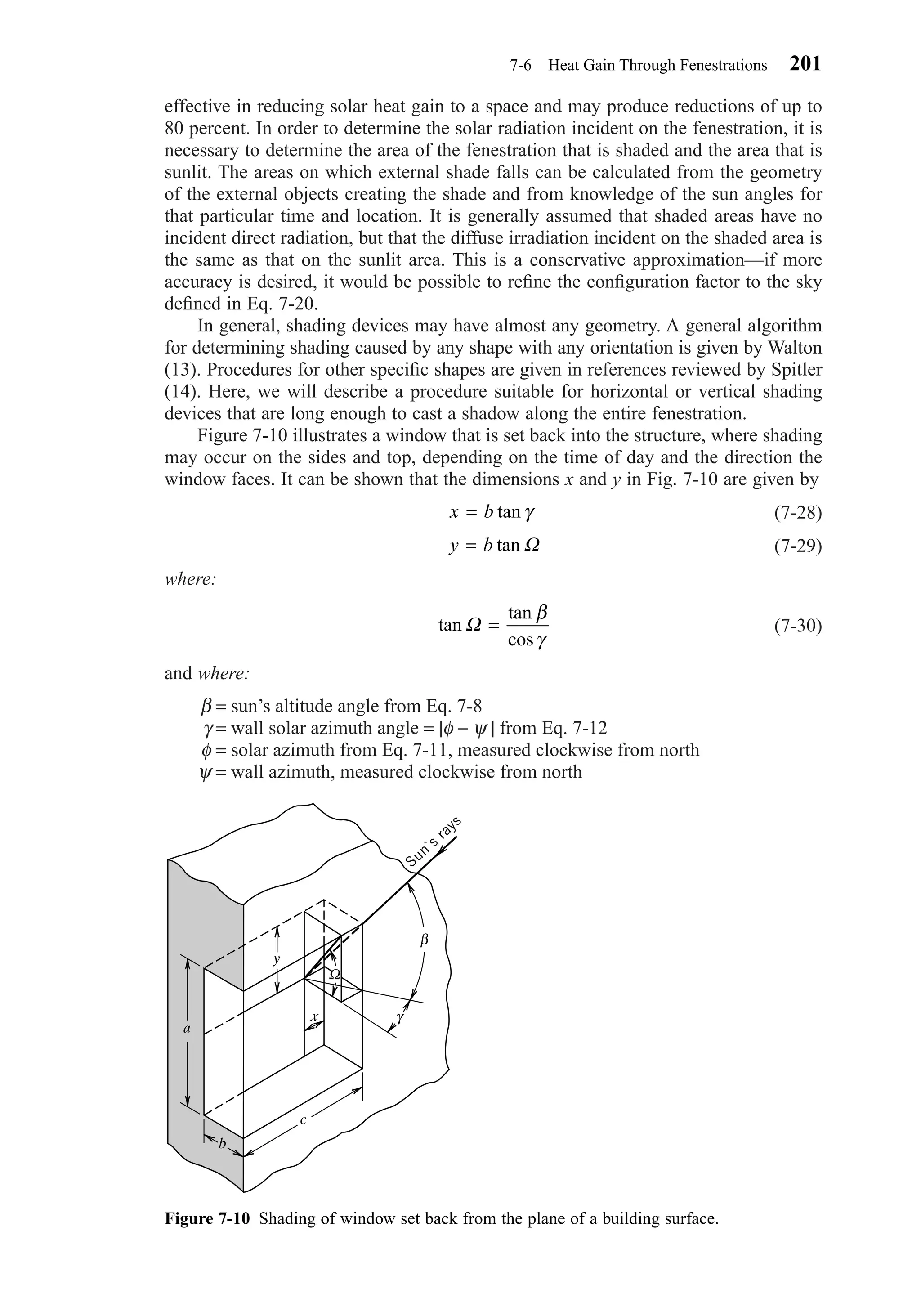
![Then, for vertical surfaces, the diffuse sky radiation is given by:
(7-22)
In determining the total rate at which radiation strikes a nonhorizontal surface at
any time, one must also consider the energy reflected from the ground or surround-
ings onto the surface. Assuming the ground and surroundings reflect diffusely, the
reflected radiation incident on the surface is:
(7-23)
where:
GR = rate at which energy is reflected onto the wall, Btu/(hr-ft2) or W/m2
GtH = rate at which the total radiation (direct plus diffuse) strikes the horizontal
surface or ground in front of the wall, Btu/(hr-ft2) or W/m2
ρg = reflectance of ground or horizontal surface
Fwg = configuration or angle factor from wall to ground, defined as the fraction
of the radiation leaving the wall of interest that strikes the horizontal
surface or ground directly
For a surface or wall at a tilt angle α to the horizontal,
(7-24)
To summarize, the total solar radiation incident on a nonvertical surface would be
found by adding the individual components: direct (Eq. 7-16a), sky diffuse (Eq. 7-18),
and reflected (Eq. 7-23):
(7-25)G G G G C F F C Gt D d R ws g wg ND= + + = + + +[ ]max(cos , ) (sin )θ ρ β0
Fwg =
−1
2
cosα
G G FR tH g wg= ρ
G
G
G
C Gd
dV
dH
NDθ =
7-5 Solar Irradiation 195
Figure 7-8 Ratio of diffuse sky radiation incident on a vertical surface to that incident on a
horizontal surface during clear days. (Reprinted by permission from ASHRAE Transactions,
Vol. 69, p. 29.)
1.4
1.2
1.0
0.8
Gdv/Gdh
0.6
0.4
0.2
–1.0 –0.8 –0.6 –0.4 –0.2 0
Cosine of sun’s incidence angle to vertical surface (cos , 0)
0.2 0.4 0.6 0.8 1.0
θ
Chapter07.qxd 6/15/04 4:10 PM Page 195](https://image.slidesharecdn.com/fayec-160521192803/75/Faye-c-mc_quiston_-_jerald_d-_parker_-_jeffrey_d-213-2048.jpg)

![The sunlit portion of the glazing has an area of
Asl,g = Ag − Ash,g = 17.81 ft2 − 11.382 ft2 = 6.43 ft2
The shaded portion of a window is assumed to receive indirect (diffuse) radiation at
the same rate as an unshaded surface, but no direct (beam) radiation.
Transmission and Absorption of Fenestration
Without Internal Shading, Simplified
In order to determine solar heat gain with the simplified procedure, it is assumed that,
based on the procedures described above, the direct irradiance on the surface (GD),
the diffuse irradiance on the surface (Gd), the sunlit area of the glazing (Asl,g), and the
sunlit area of the frame (Asl,f) are all known. In addition, the areas of the glazing (Ag)
and frame (Af) and the basic window properties must be known.
The solar heat gain coefficient of the frame (SHGCf) may be estimated as
(7-31)
where Aframe is the projected area of the frame element, and Asurf is the actual surface
area. αs
f is the solar absorptivity of the exterior frame surface (see Table 7-1). Uf is the
U-factor of the frame element (see Table 5-6); hf is the overall exterior surface con-
ductance (see Table 5-2). If other frame elements like dividers exist, they may be ana-
lyzed in the same way.
The solar heat gain coefficient of the glazing may be taken from Table 7-3 for a
selection of sample windows. For additional windows, the reader should consult the
ASHRAE Handbook, Fundamentals Volume (5) as well as the WINDOW software
(12). There are actually two solar heat gain coefficients of interest, one for direct radi-
ation at the actual incidence angle (SHGCgD) and a second for diffuse radiation
(SHGCgd). SHGCgD may be determined from Table 7-3 by linear interpolation. Val-
ues of SHGCgd may be found in the column labeled “Diffuse.”
Once the values of SHGCf, SHGCgD, and SHGCgd have been determined, the total
solar heat gain of the window may be determined by applying direct radiation to the sun-
lit portion of the fenestration and direct and diffuse radiation to the entire fenestration:
(7-32)
To compute the total heat gain through the window, the conduction heat gain must be
added, which is estimated as
(7-33)
where U for the fenestration may be taken from Table 5-5, the ASHRAE Handbook,
Fundamentals Volume (5), or the WINDOW 5.2 software (12); and (to − ti) is the
outdoor–indoor temperature difference.
EXAMPLE 7-6
Consider the 4 ft high × 5 ft wide, fixed (inoperable) double-glazed window, facing
southwest from Example 7-5. The glass thickness is in., the two panes are separated
by a in. air space, and surface 2 (the inside of the outer pane) has a low-e coating
with an emissivity of 0.1. The frame, painted with white acrylic paint, is aluminum
1
4
1
8
˙ ( )q U t tCHG o i= −
˙ , ,q SHGC A SHGC A G SHGC A SHGC A GSHG gD sl g f sl f D gd g f f d= +[ ] + +[ ]θ θ
SHGC f f
s f frame
f surf
U A
h A
=
α
7-6 Heat Gain Through Fenestrations 203
Chapter07.qxd 6/15/04 4:10 PM Page 203](https://image.slidesharecdn.com/fayec-160521192803/75/Faye-c-mc_quiston_-_jerald_d-_parker_-_jeffrey_d-221-2048.jpg)
![with thermal break; the spacer is insulated. The outer layer of glazing is set back from
the edge of the frame in. On July 21 at 3:00 P.M. solar time at 40 deg N latitude, the
incident angle is 54.5 deg, the incident direct irradiation is 155.4 Btu/hr-ft2, and the
incident diffuse irradiation is 60.6 Btu/hr-ft2. Find the solar heat gain of the window.
SOLUTION
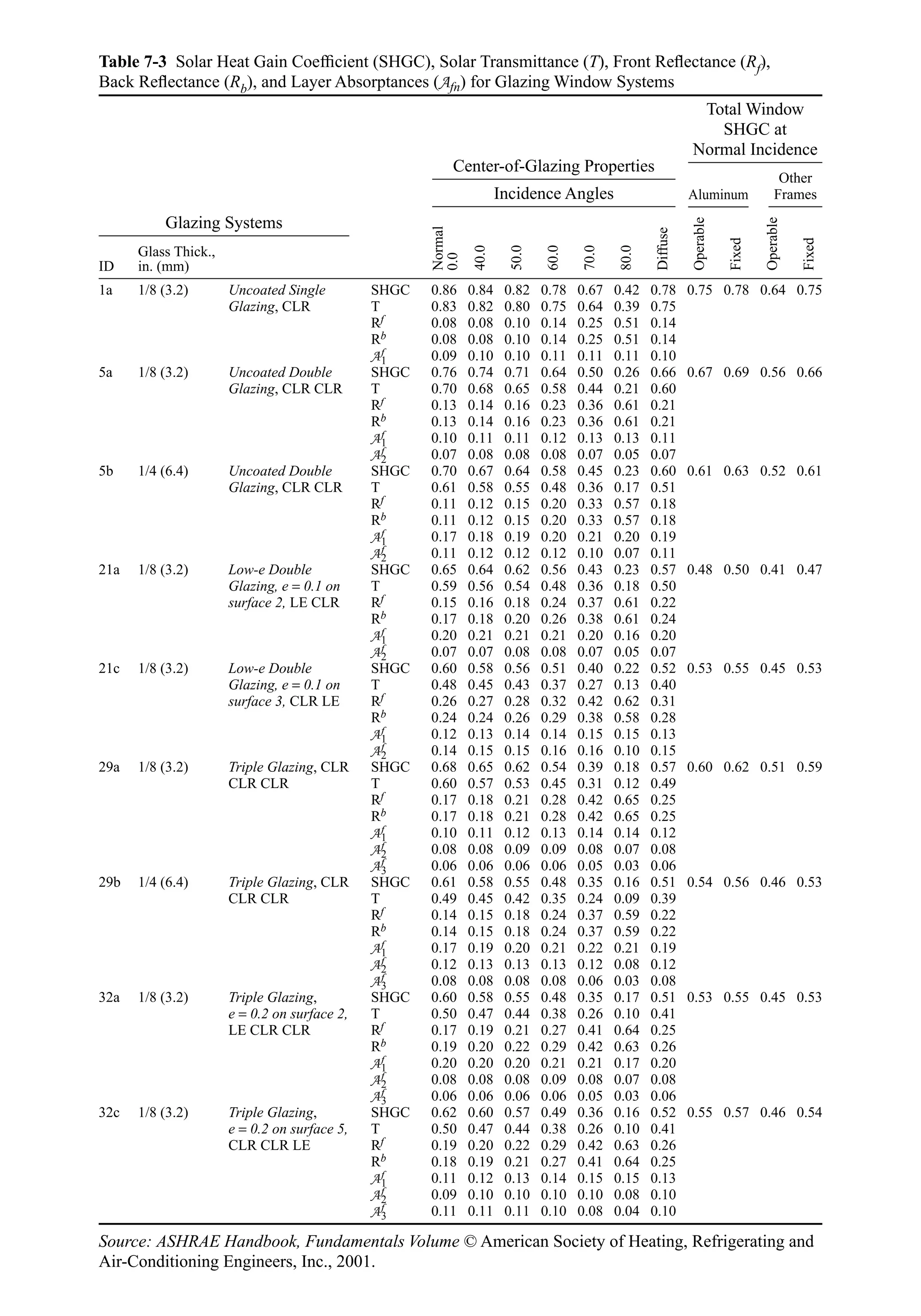
The window corresponds to ID 21a in Table 7-3 and SHGCgD is found to be 0.59;
SHGCgd is 0.57. The frame U-factor may be determined from Table 5-6 to be 1.04
Btu/hr-ft2-F. The solar absorptance of white acrylic paint, from Table 7-1, is 0.26. The
outside surface conductance, from Table 5-2, is 4.0 Btu/hr-ft2-F. The projected area of
the frame is 2.63 ft2; the actual surface area, 2.81 ft2, is slightly larger, because the
glass is set back in. from the outer edge of the frame. SHGCf may be estimated with
Eq. 7-31
Then, from Eq. 7-32, the solar heat gain may be estimated:
Transmission and Absorption of Fenestration
Without Internal Shading, Detailed
In this section, procedures for determining the direct and diffuse solar radiation trans-
mitted and absorbed by a window will be described. Absorbed solar radiation may
flow into the space or back outside. Therefore, procedures for estimating the inward
flowing fraction will also be discussed.
The transmitted solar radiation depends on the angle of incidence—the transmit-
tance is typically highest when the angle is near zero, and falls off as the angle of inci-
dence increases. Transmittances are tabulated for a range of incidence angles for
several different glazing types in Table 7-3. In addition, the transmittance for diffuse
radiation Td, assuming it to be ideally diffuse (uniform in all directions), is also given.
To determine the transmittance TDθ for any given incidence angle, it is permissible to
linearly interpolate between the angles given in Table 7-3. Alternatively, the coeffi-
cients tj in Eq. 7-34 might be determined with an equation-fitting procedure to fit the
transmittance data. Then, Eq. 7-34 could be used to directly determine the direct trans-
mittance for any given angle.
(7-34)
Once the direct transmittance has been determined, the transmitted solar radiation
may be computed by summing the contributions of the direct radiation (only incident
on the sunlit area of the glazing) and the diffuse radiation (assumed incident over the
entire area of the glazing) as
(7-35)˙ , ,q T G A T G ATSHG g D D sl g d d g= +θ θ θ
T tD j
j
j
θ θ= [ ]
=
∑ cos
0
5
˙ . . . . . . . . . .
.
qSHG = × + ×[ ] + × + ×[ ]
=
0 59 6 43 0 063 1 41155 4 0 57 17 81 0 063 2 63 60 6
1228 6 or 1230
Btu
hr
SHGCf =
×
×
=0 26
1 04 2 63
4 0 2 81
0 063.
. .
. .
.
1
8
1
8
204 Chapter 7 Solar Radiation
Chapter07.qxd 6/15/04 4:10 PM Page 204](https://image.slidesharecdn.com/fayec-160521192803/75/Faye-c-mc_quiston_-_jerald_d-_parker_-_jeffrey_d-222-2048.jpg)
![where qTSHG,g is the total transmitted solar radiation through the glazed area of
the fenestration, Asl,g is the sunlit area of the glazing, and Ag is the area of the glazing.
The absorbed solar radiation also depends on the incidence angle, and layer-by-
layer absorptances are also tabulated in Table 7-3. It should be noted that absorptances
apply to the solar radiation incident on the outside of the window; for the second and
third layers, the absorbed direct solar radiation in that layer would be calculated by
multiplying the absorptance by GDθ. The total solar radiation absorbed by the K glaz-
ing layers is then given by
(7-36)
where the absorptances for the kth layer, Af
k Dθ, are interpolated from Table 7-3. The
superscript f specifies that the absorptances apply for solar radiation coming from the
front or exterior of the window, not for reflected solar radiation coming from the back
of the window.
It is then necessary to estimate the inward flowing fraction, N. A simple estimate
may be made by considering the ratio of the conductances from the layer to the inside
and outside. For the kth layer, the inward flowing fraction is then given by
(7-37)
where U is the U-factor for the center-of-glazing and ho,k is the conductance between
the exterior environment and the kth glazing layer. Then the inward flowing fraction
for the entire window is given by
(7-38)
In addition to the solar radiation absorbed by the glazing, a certain amount is also
absorbed by the frame and conducted into the room. It may be estimated as
(7-39)
where Af is the projected area of the frame element, and Asurf is the actual surface
area. αs
f is the solar absorptivity of the exterior frame surface. Uf is the U-factor of
the frame element, and hf is the overall surface conductance. If other frame elements
such as dividers exist, they may be analyzed in the same way.
Finally, the total absorbed solar radiation for the fenestration is
(7-40)
EXAMPLE 7-7
Repeat Example 7-6, using the detailed analysis.
SOLUTION
To analyze the glazing, we will need to know the transmittance and layer-by-layer
absorptances for an incidence angle of 54.5 deg. By interpolating from Table 7-3, we
˙ ˙ ˙, , ,q N q qASHG gf ASHG g ASHG f= +
˙ , ,q G A G A
U A
h AASHG f D sl f d f f
s f f
f surf
= +[ ]
θ θ α
N
G N G N
G G
D k D
f
k d k d
f
k
K
k
K
k
D d
=
+
+
==
∑∑θ θ θ
θ θ
A A
11
N
U
hk
o k
=
,
˙ , ,q G A G AASHG g D sl g k D
f
k
K
d g k d
f
k
K
= +
= =
∑ ∑θ θ θA A
1 1
7-6 Heat Gain Through Fenestrations 205
Chapter07.qxd 6/15/04 4:10 PM Page 205](https://image.slidesharecdn.com/fayec-160521192803/75/Faye-c-mc_quiston_-_jerald_d-_parker_-_jeffrey_d-223-2048.jpg)
![find TDθ = 0.51, Af
1Dθ = 0.21, and Af
2Dθ = 0.08. The diffuse properties are Td = 0.50,
Af
1d = 0.20, and Af
2d = 0.07. Then, the transmitted solar radiation may be found with
Eq. 7-35:
And the absorbed radiation may be found:
The U-factor for the center of glass is 0.42 Btu/hr-ft2-F from Table 5-5a. In order to
estimate the fraction of absorbed radiation, it is necessary to estimate the inward flow-
ing fraction. First, the inward flowing fraction must be estimated for each layer. To
use Eq. 7-37 it is necessary to estimate the conductance between the outer pane (layer
1) and the outside air, and the conductance between the inner pane (layer 2) and the
outside air. For layer 1, the conductance is simply the exterior surface conductance,
For layer 2, the conductance between layer 2 and the outside air may be estimated by
assuming that the resistance between the inner pane and the outside air is equal to the
total resistance of the window minus the resistance from the inner pane to the inside
air. (The resistances of the glass layers are assumed to be negligible.) Taking the value
of hi from Table 5-2a:
Then, the conductance from the inner pane to the outdoor air is:
The inward flowing fraction for the inner pane is:
As expected, much more of the absorbed radiation from the inner pane flows inward
than that absorbed by the outer pane. Now that N1 and N2 have been calculated, the
inward flowing fraction can be determined with Eq. 7-38:
The solar heat gain absorbed by the frame and conducted into the room may be esti-
mated with Eq. 7-39. Note that it is analogous to the calculation and use of the SHGCf
in the simplified procedure.
˙ . . . . .
. .
. .
.,qASHG f = × + ×[ ]
×
×
=155 4 1 41 60 6 2 63 0 26
1 04 2 63
4 0 2 81
23 9
Btu
hr
N =
× + × + × + ×[ ]
+
=
155 4 0 21 0 11 0 08 0 71 60 6 0 20 0 11 0 07 0 71
155 4 60 6
0 08
. ( . . . . ) . ( . . . . )
. .
.
N
U
ho
2
2
0 42
0 59
0 71= = =
,
.
.
.
Btu/hr-ft -F
Btu/hr-ft - F
2
2
h
Ro
o
,
,
.2
2
1
0 59= =
Btu
hr-ft -F2
R
U ho
i
,
. .
.2
1 1 1
0 42
1
1 46
1 7= − = − =
Btu
hr-ft -F
Btu
hr-ft -F
hr-ft -F
Btu
2 2
2
N
U
ho
1
1
0 42
4 0
0 11= = =
,
.
.
.
Btu/hr-ft -F
Btu/hr-ft -F
2
2
˙ . . ( . . ) . . ( . . )
.
,qASHG g = × × + + × × +
=
155 4 6 43 0 21 0 08 60 6 17 81 0 20 0 07
581 2 or 580 Btu/hr
˙ . . . . . . .,qTSHG g = × × + × × =0 51 155 4 6 43 0 50 60 6 17 81 1049 2 or 1050
Btu
hr
206 Chapter 7 Solar Radiation
Chapter07.qxd 6/15/04 4:10 PM Page 206](https://image.slidesharecdn.com/fayec-160521192803/75/Faye-c-mc_quiston_-_jerald_d-_parker_-_jeffrey_d-224-2048.jpg)
![The absorbed heat gain may now be calculated with Eq. 7-40:
The total solar heat gain is the sum of the transmitted and absorbed components, or
1119.6 Btu/hr.
Transmission and Absorption of Fenestration
with Internal Shading, Simplified
Internal shading, such as Venetian blinds, roller shades, and draperies, further com-
plicate the analysis of solar heat gain. Shading devices are successful in reducing solar
heat gain to the degree that solar radiation is reflected back out through the window.
Solar radiation absorbed by the shading device will be quickly released to the room.
Limited availability of data precludes a very detailed analysis, and angle of incidence
dependence is usually neglected. To calculate the effect of internal shading, it is con-
venient to recast Eq. 7-32 to separate the heat gain due to the glazing and frame. Then,
the solar radiation transmitted and absorbed by the glazing is multiplied by an interior
solar attenuation coefficient (IAC).
(7-41)
Interior solar attenuation coefficients for Venetian blinds and roller shades may be
found in Table 7-4. Since the effect of the shading device depends partly on the win-
dow, the values of IAC given in Table 7-4 depend on both the shading device and the
type of glazing, characterized by configuration and SHGC at normal incidence.
For draperies, the IAC depends on the color and weave of the fabric. Although
other variables also have an effect, reasonable correlation has been obtained using
only color and openness of the weave. Figure 7-12 may be used to help characterize
openness. Openness is classified as open, I; semiopen, II; and closed, III. Color is clas-
sified as dark, D; medium, M; and light, L. A light-colored, closed-weave material
would then be classified IIIL. Once the category has been established, an index letter
(A to J) may be read and used to determine the IAC from Table 7-5. For any category,
several index letters may be chosen, and judgment based on the color and weave is
required in making a final selection.
EXAMPLE 7-8
If an opaque white roller shade were added to the window in Example 7-6, what would
be the effect on the solar heat gain?
SOLUTION
From Table 7-4, the interior solar attenuation coefficient for an opaque white roller
shade installed on a residential double-pane window is 0.41. From Eq. 7-41, the result-
ing solar heat gain may be calculated:
˙ . . . . . .
. . . . . . . .
qSHG = × × + × ×[ ]
+ × × + × ×[ ] =
0 063 1 41 155 4 0 063 2 63 60 6
0 59 6 43 155 4 0 57 17 81 60 6 0 41 493 9 490or Btu/hr
˙ ,
,
q SHGC A G SHGC A G
SHGC A G SHGC A G IAC
SHG f sl f D f f d
gD sl g D gd g d
= +[ ]
+ +[ ]
θ θ
θ θ
˙ . . . .,qASHG gf = × + =0 08 581 2 23 9 70 4 Btu/hr
7-6 Heat Gain Through Fenestrations 207
Chapter07.qxd 6/15/04 4:10 PM Page 207](https://image.slidesharecdn.com/fayec-160521192803/75/Faye-c-mc_quiston_-_jerald_d-_parker_-_jeffrey_d-225-2048.jpg)
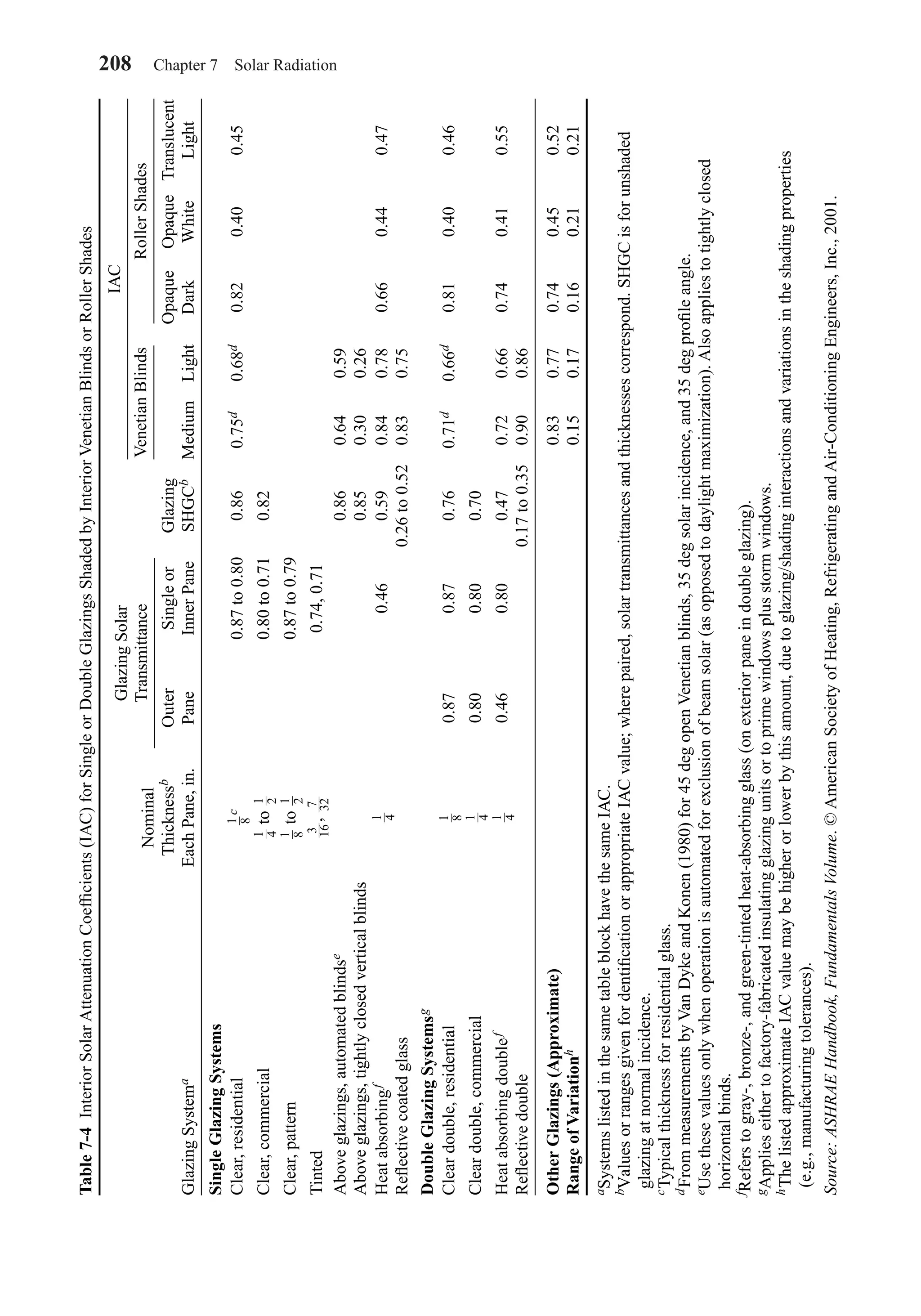
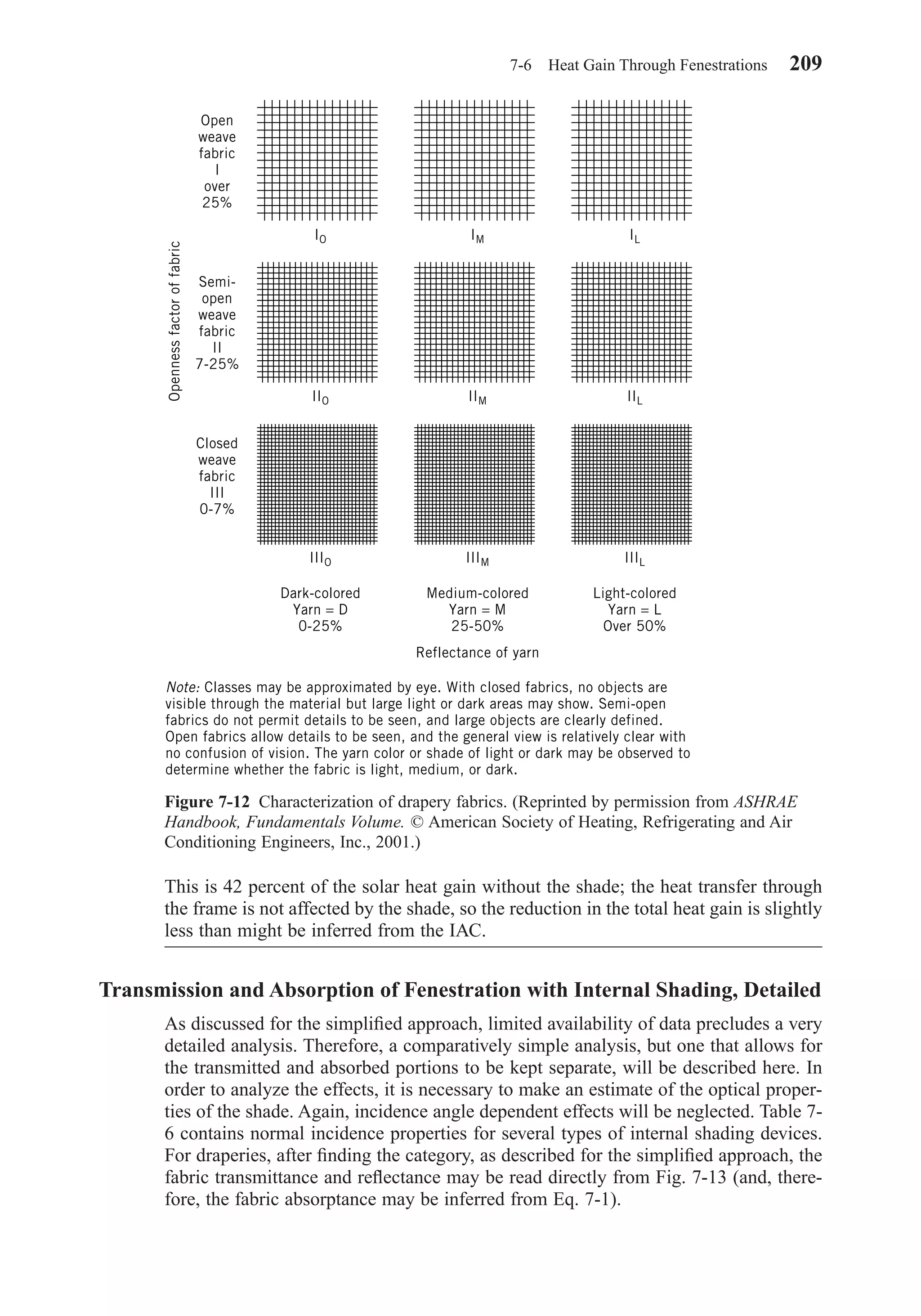
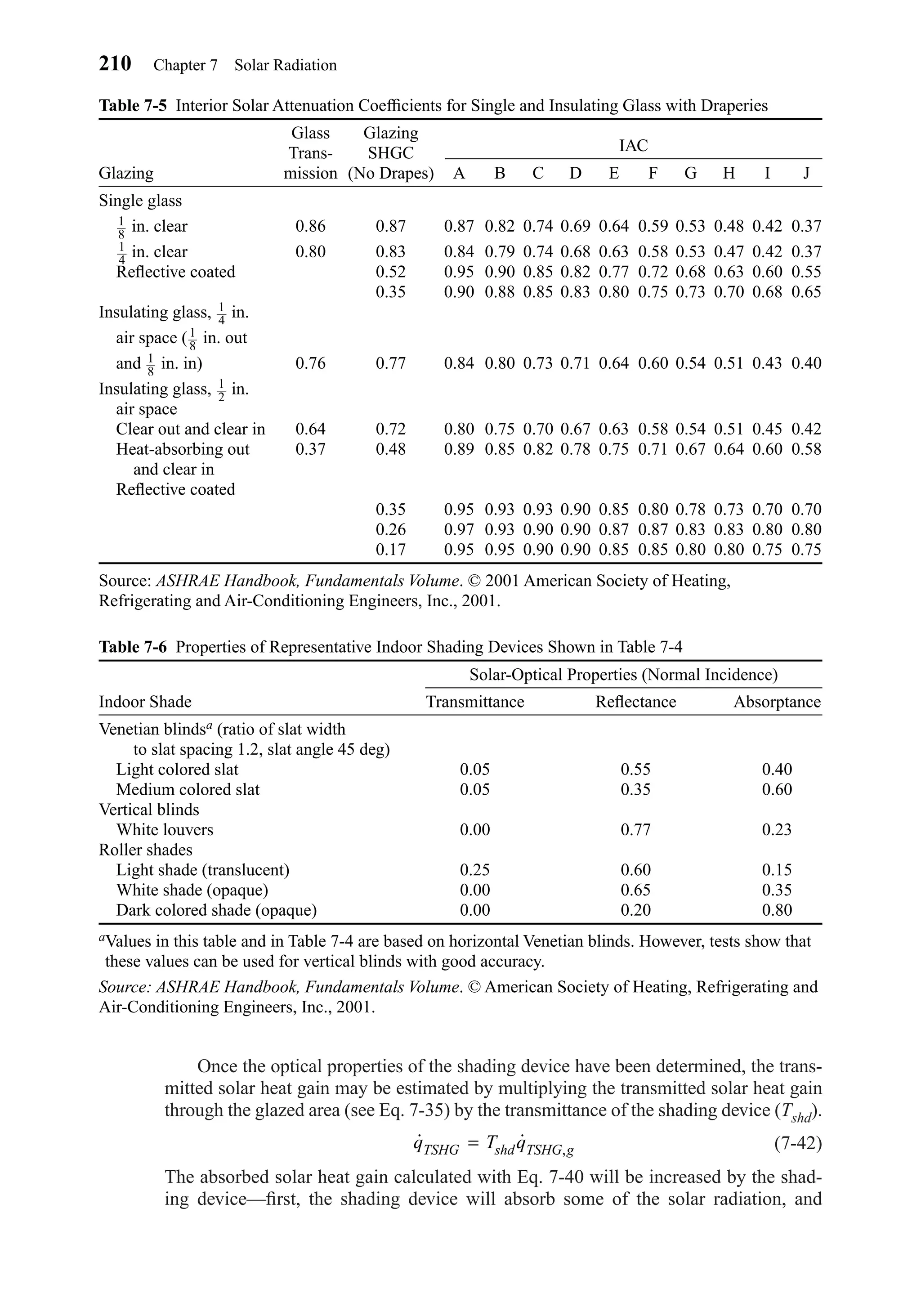

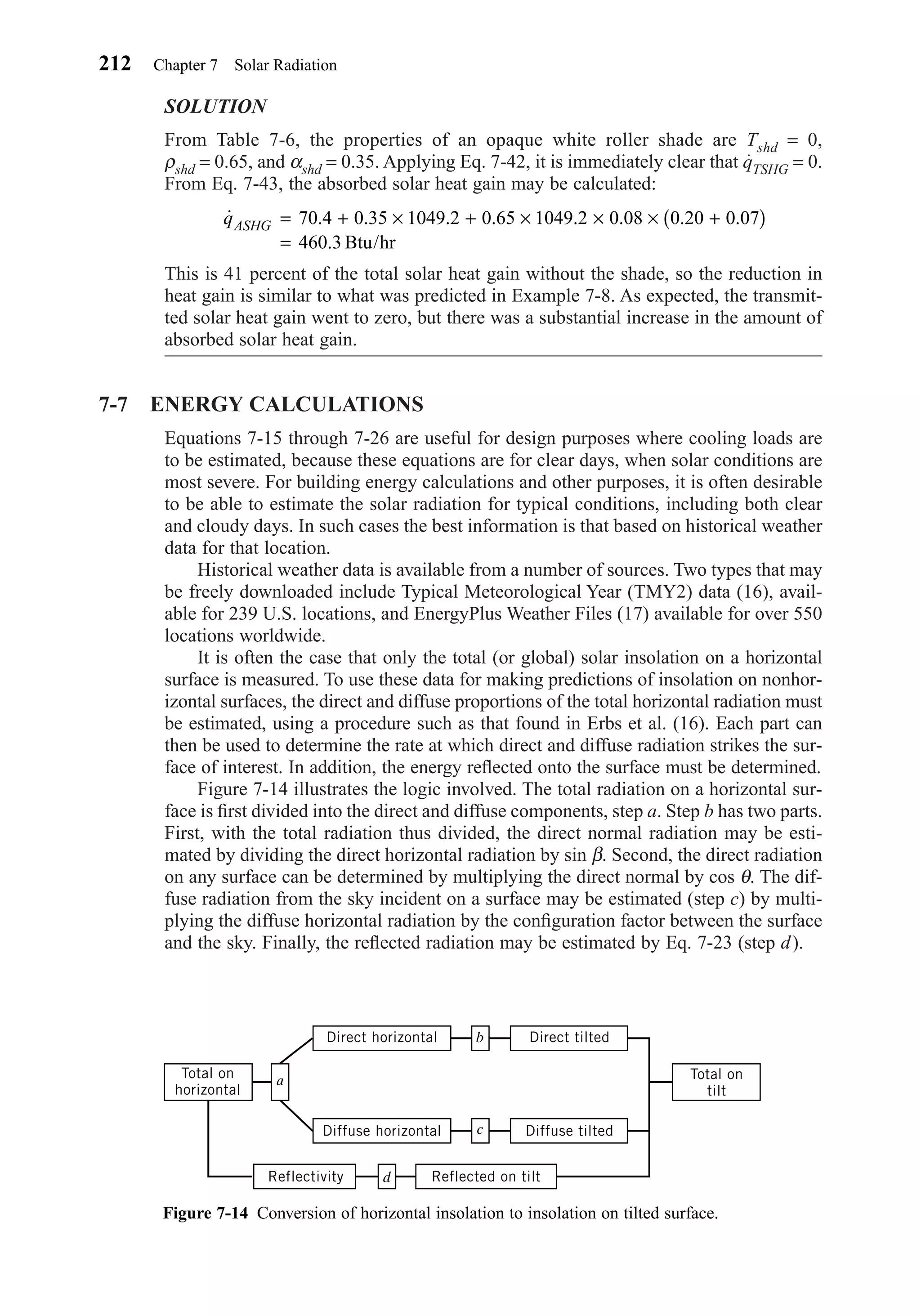

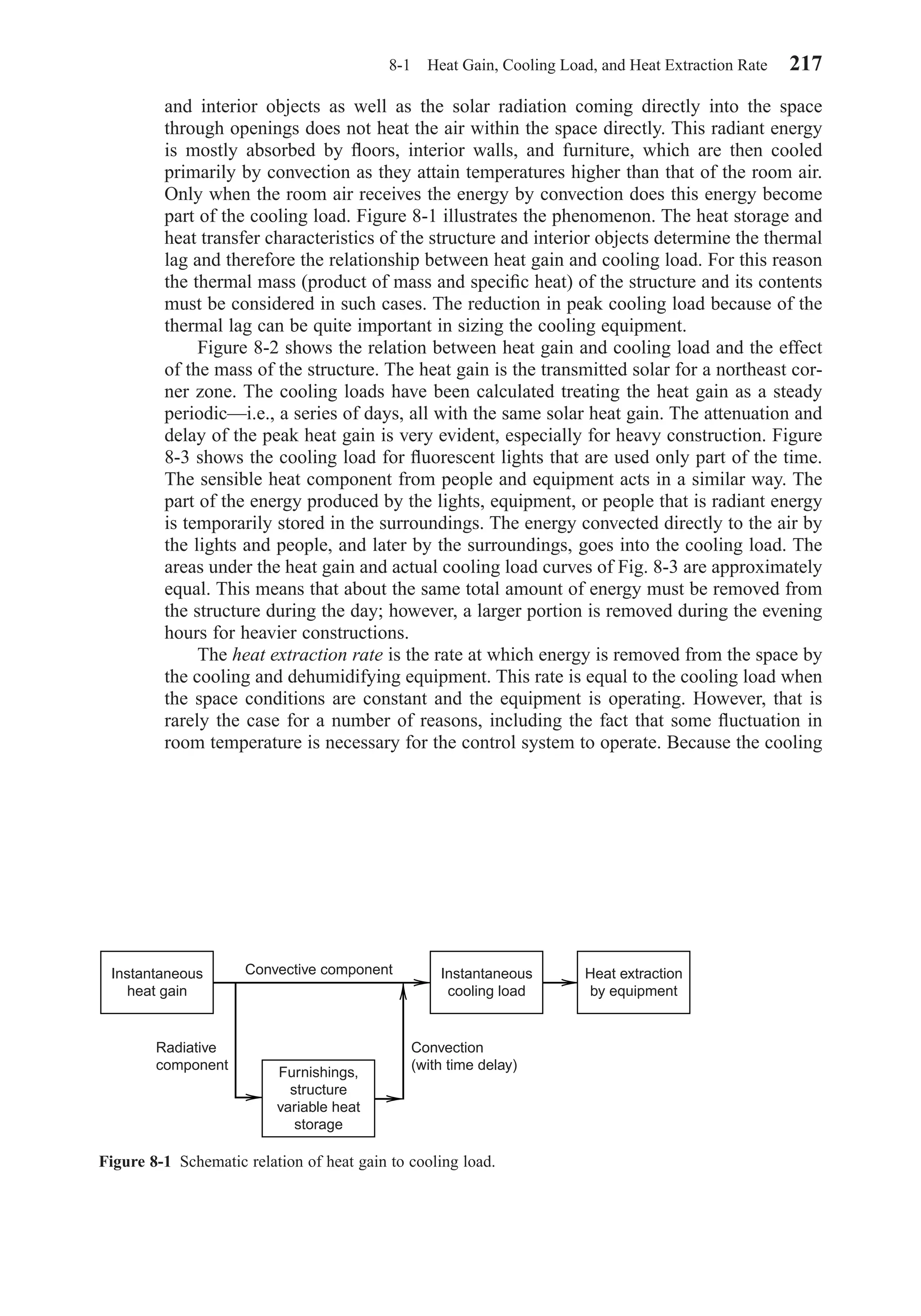
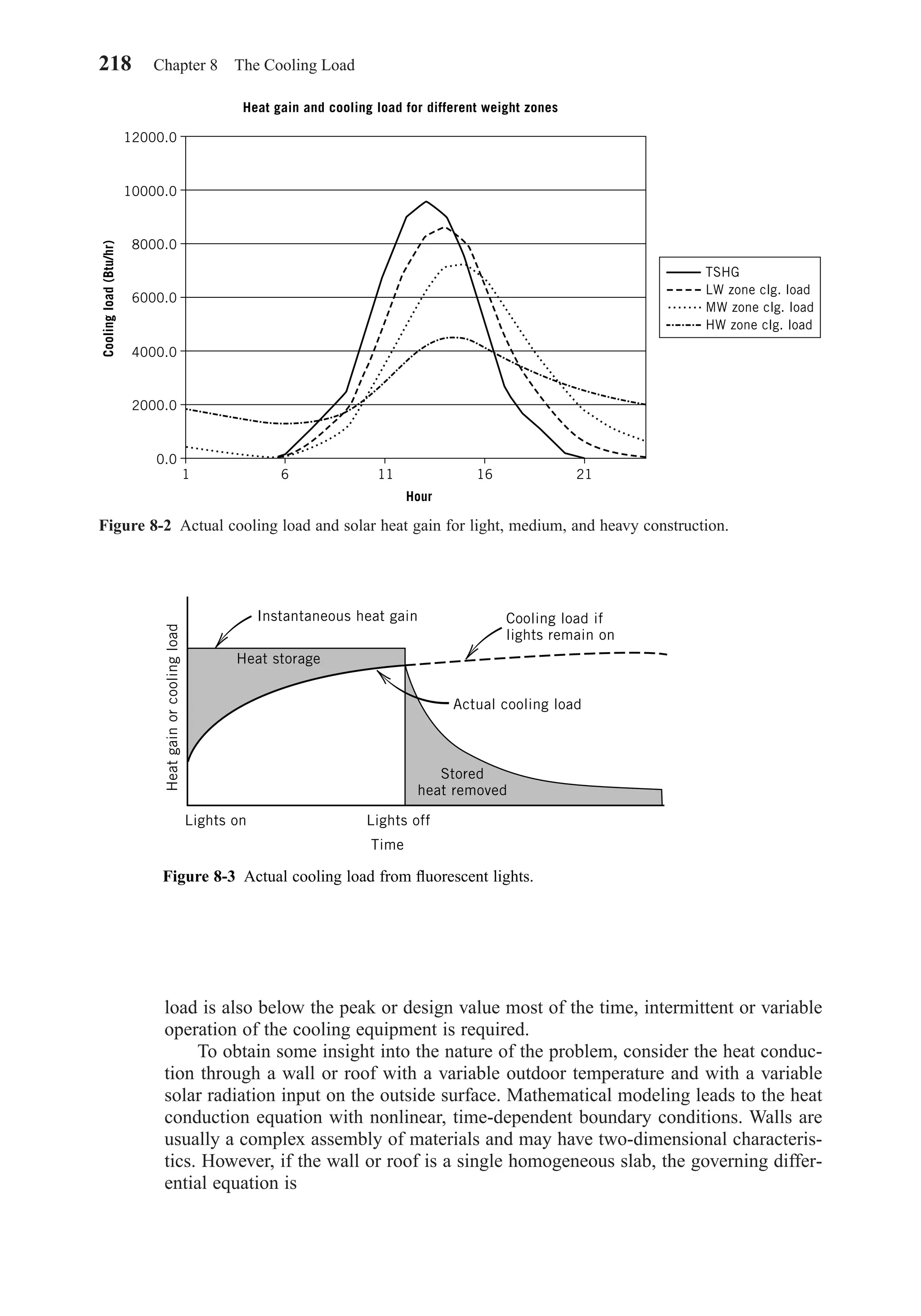
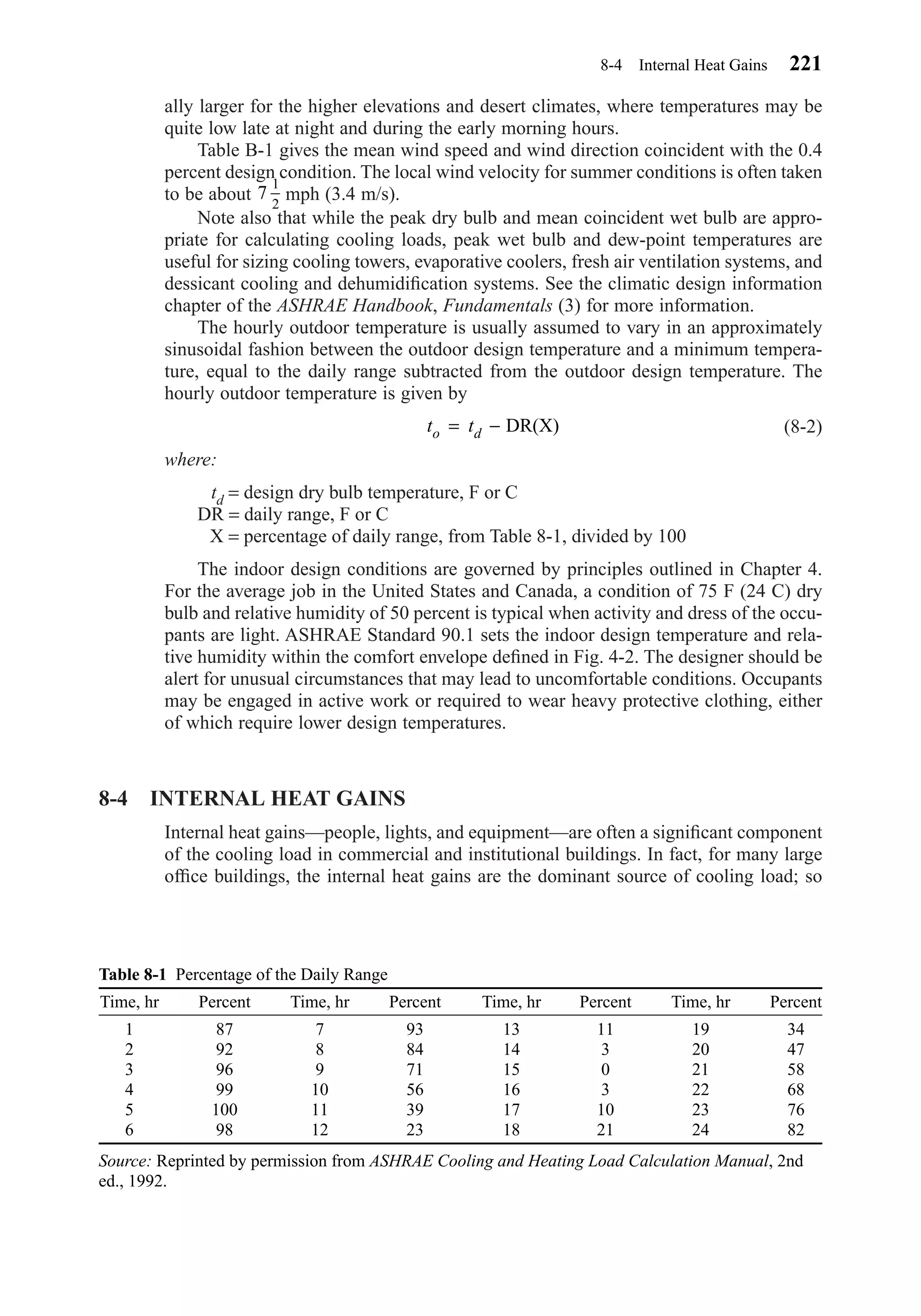
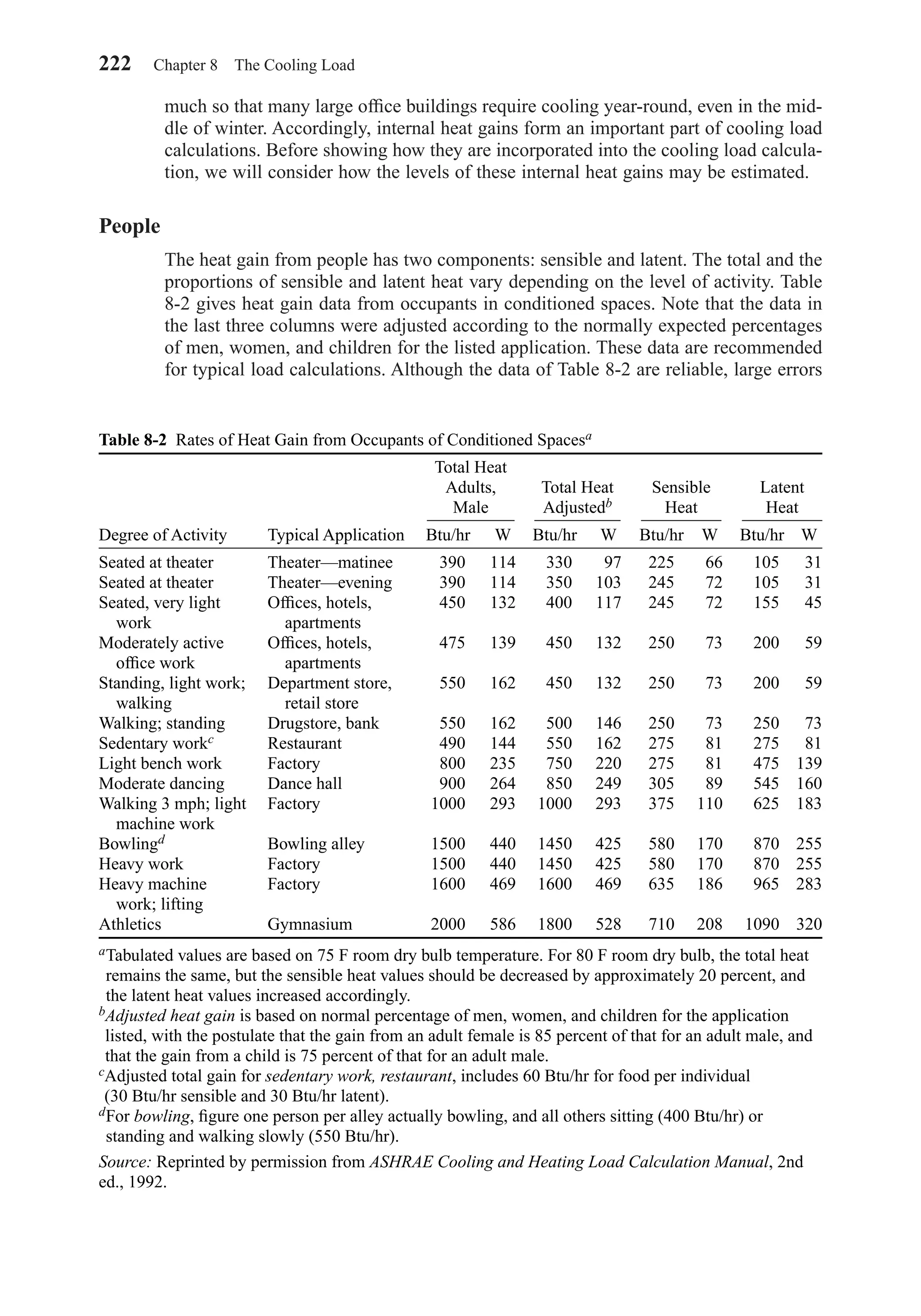
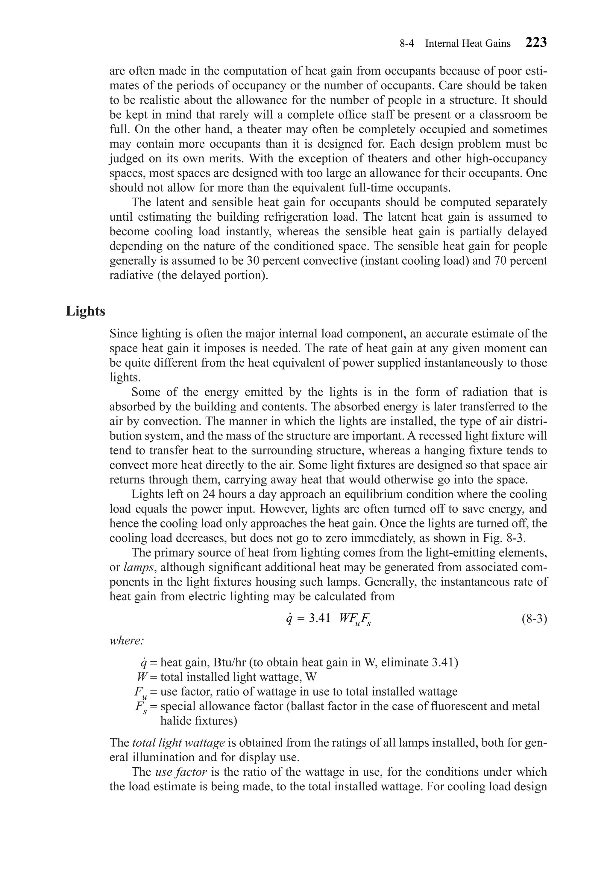

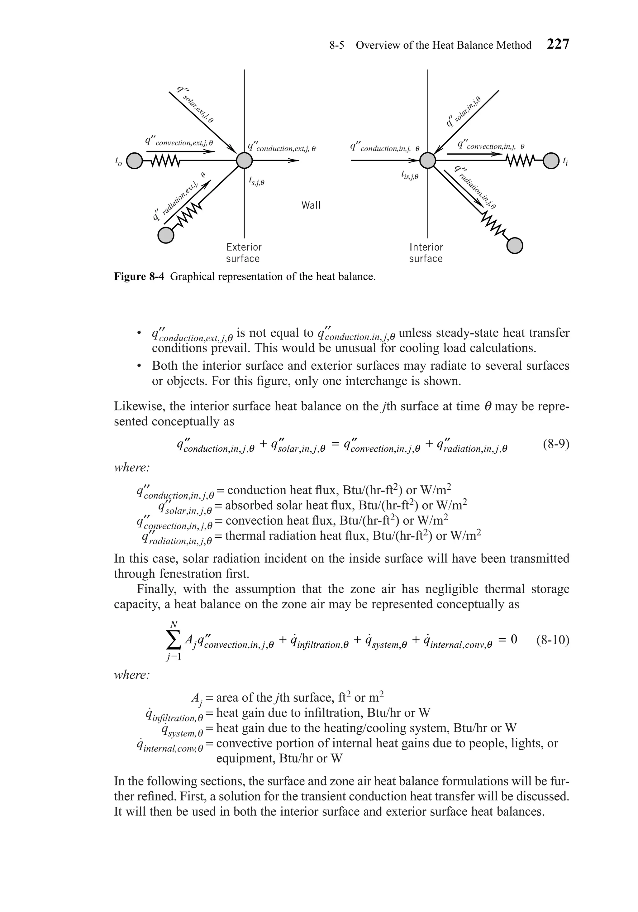
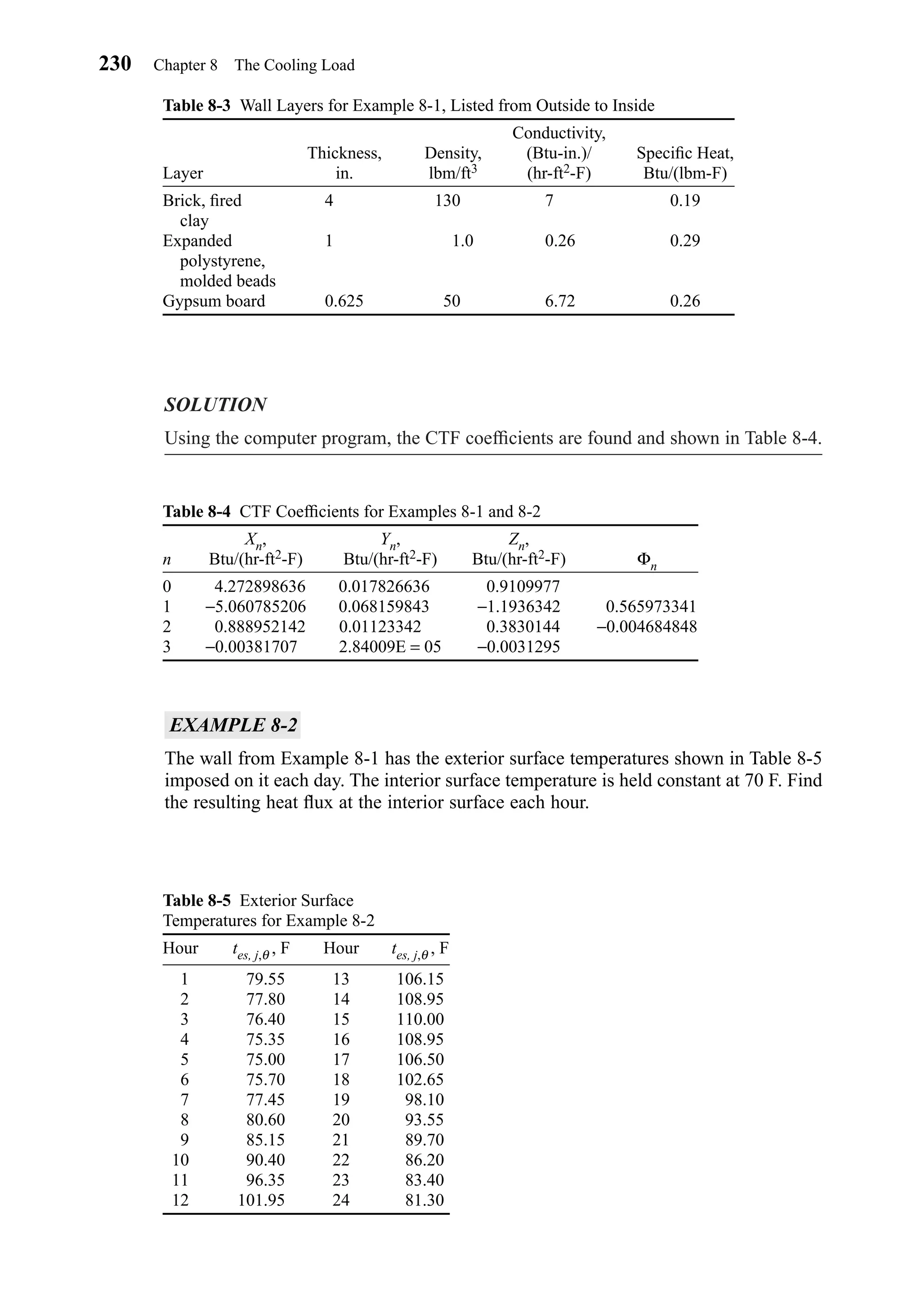
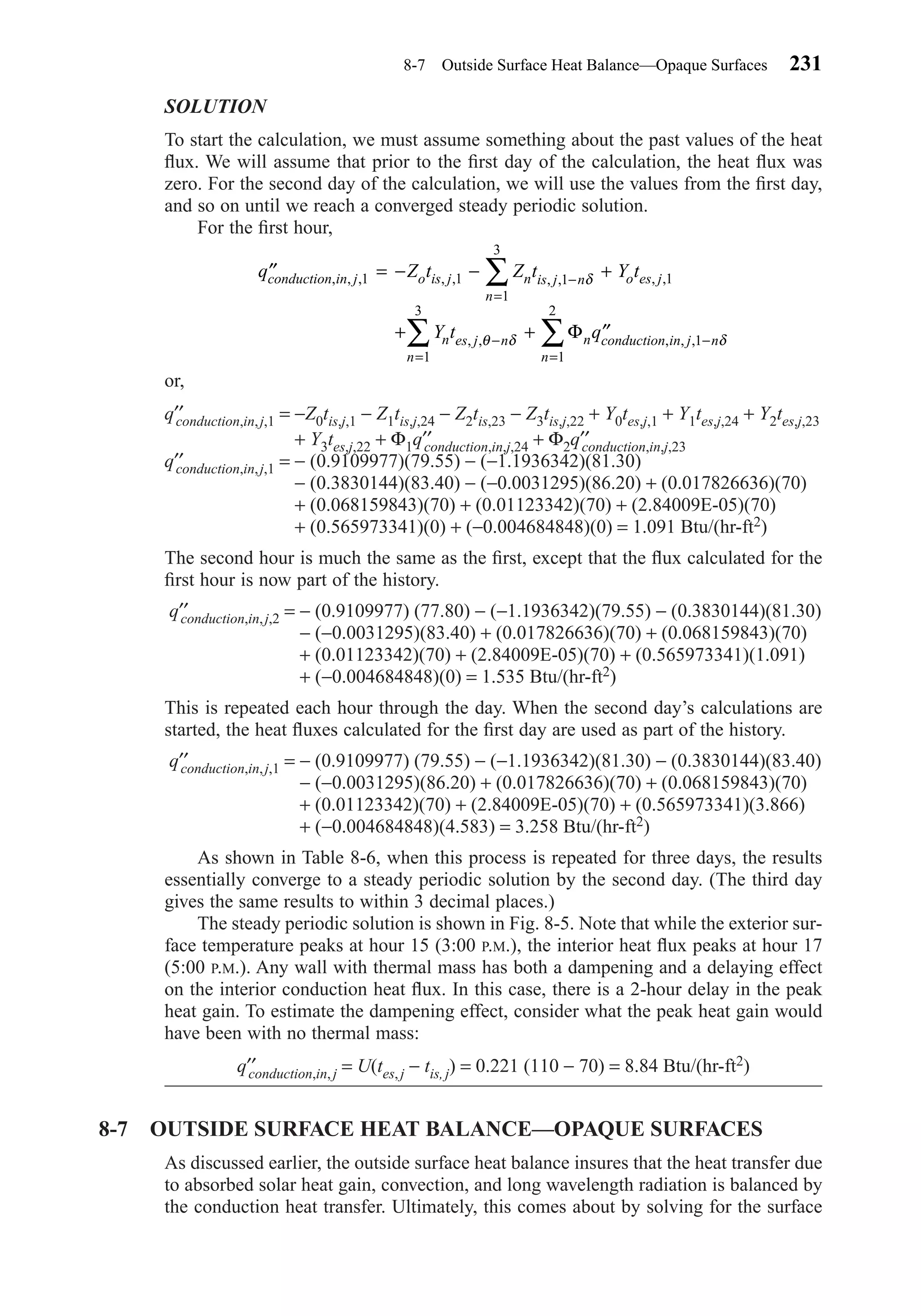
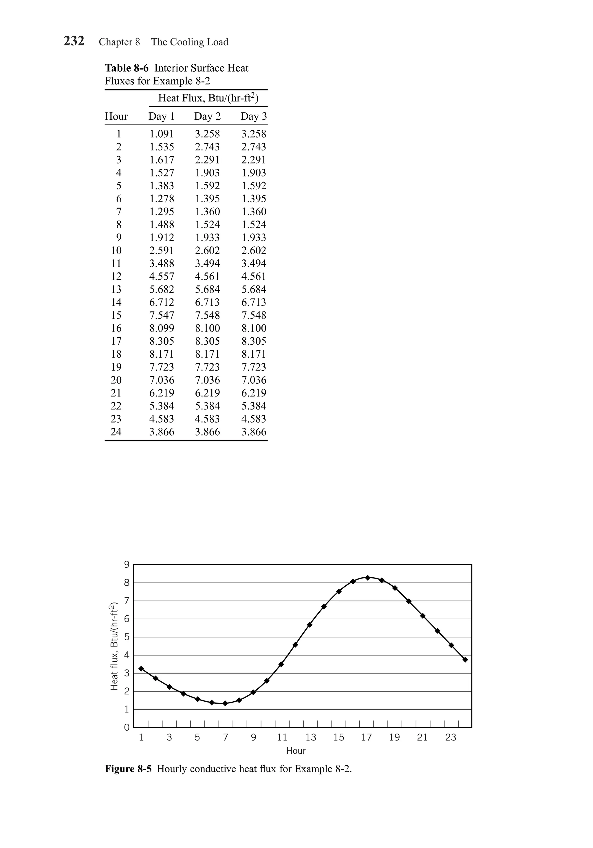
![temperature that results in a heat balance being achieved. This section will discuss
how each heat transfer mechanism is modeled. For each mechanism, there are a num-
ber of possible models that could be used, ranging from very simple to very complex.
Selecting a suitable model can be challenging—the level of sophistication of the
model may depend on the problem at hand. We will follow the approach of selecting
a reasonably simple model for each heat transfer mechanism, and refer the reader to
other sources for more sophisticated and accurate models.
Absorbed Solar Heat Gain
Absorbed solar heat gain is calculated using the principles and algorithms described
in Chapter 7. Specifically,
(8-16)
where:
α = solar absorptivity of the surface, dimensionless
Gt = total solar irradiation incident on the surface, Btu/(hr-ft2) or W/m2
Typically, for design load calculations, the irradiation is calculated with the ASHRAE
Clear Sky Model described in Chapter 7. Since the irradiation must be calculated for
a specific time, yet represent the entire hour, it is usually calculated at the half hour.
Exterior Convection
Convection to exterior surfaces may be represented with a range of models, all of
which involve the use of a convection coefficient:
(8-17)
where hc is the convection coefficient.
McClellan and Pedersen (20) give a brief review. Given the very complex wind-
driven and buoyancy-driven air flows around a building, a convective heat transfer
model might be very complex and difficult to use. A correlation recently developed by
Yazdanian and Klems (21) seems to strike a reasonable balance between accuracy and
ease-of-use for low-rise buildings. The correlation takes the form
(8-18a)
where:
Ct = turbulent natural convection constant, given in Table 8-7
∆t = temperature difference between the exterior surface and the outside air, F or C
a, b = constants given in Table 8-7
Vo = wind speed at standard conditions, mph or m/s
For high-rise buildings, Loveday and Taki (22) recommend the correlation:
(8-18b)
where:
C
Vs
= =
=
−
−
1 97 16 70 5
0 5
. ( ) ..
.
Btu
hr-ft -F
mph
W
m K
m
s
wind speed near surface, mph or m/s
2 2
h CVc s= 0 5.
h C t aVc t o
b= [ ] + [ ]( ) /∆ 1 3 2 2
′′ = −q h t tconvection ext j c o os j, , , , ,( )θ θ
′′ =q Gsolar ext j t, , ,θ α
8-7 Outside Surface Heat Balance—Opaque Surfaces 233
Chapter08.qxd 6/15/04 4:06 PM Page 233](https://image.slidesharecdn.com/fayec-160521192803/75/Faye-c-mc_quiston_-_jerald_d-_parker_-_jeffrey_d-251-2048.jpg)
![The correlation was based on windspeeds between 0.5 mph (0.2 m/s) and 9 mph
(4 m/s). Loveday and Taki do not make a recommendation for windspeeds below
0.5 mph (0.2 m/s), but a minimum convection coefficient of 1.3 Btu/hr-ft2-F or
7.5 W/m2K might be inferred from their measurements.
Exterior Radiation
Long wavelength (thermal) radiation to and from exterior surfaces is also a very com-
plex phenomenon. The exterior surfaces radiate to and from the surrounding ground,
vegetation, parking lots, sidewalks, other buildings, and the sky. In order to make the
problem tractable, a number of assumptions are usually made:
• Each surface is assumed to be opaque, diffuse, and isothermal and to have uni-
form radiosity and irradiation.
• Each surface is assumed to be gray, having a single value of absorptivity and
emissivity that applies over the thermal radiation spectrum. (The surface may
have a different value of absorptivity that applies in the solar radiation spectrum.)
• Radiation to the sky, where the atmosphere is actually a participating medium,
may be modeled as heat transfer to a surface with an effective sky temperature.
• Lacking any more detailed information regarding surrounding buildings, it is
usually assumed that the building sits on a flat, featureless plane, so that a ver-
tical wall has a view factor between the wall and the ground of 0.5, and
between the wall and the sky of 0.5.
• Without a detailed model of the surrounding ground, it is usually assumed to
have the same temperature as the air. Obviously, for a wall with a significant
view to an asphalt parking lot, the ground temperature would be somewhat
higher.
With these assumptions, the net long wavelength radiation into the surface is given by
(8-19)
where:
⑀ = surface long wavelength emissivity
σ = Stefan–Boltzmann constant = 0.1714 × 10⁻⁸ Btu/(hr-ft2-R4)
= 5.67 × 10⁻⁸ W/(m2-K4)
Fs−g = view factor from the surface to the ground
Fs−sky = view factor from the surface to the sky
tg = ground temperature, R or K
tsky = effective sky temperature, R or K
tes, j,θ = surface temperature, R or K
′′ = −( )+ −( )[ ]− −q F t t F t tradiation ext j s g g es j s sky sky es j, , , , , , ,θ θ θσ⑀ 4 4 4 4
234 Chapter 8 The Cooling Load
Table 8-7 Convection Correlation Coefficients for MoWitt Model
Btu/ W/ Btu/ W/
Direction (hr-ft2-F4/3) (m2K4/3) (hr-ft2-F-mph) (m2-K-m/s) b
Windward 0.096 0.84 0.203 2.38 0.890
Leeward 0.096 0.84 0.335 2.86 0.617
Ct a
Chapter08.qxd 6/15/04 4:06 PM Page 234](https://image.slidesharecdn.com/fayec-160521192803/75/Faye-c-mc_quiston_-_jerald_d-_parker_-_jeffrey_d-252-2048.jpg)
![(8-29)
This is a well-insulated surface under a noonday sun in June, so an initial guess of
tes, j,θ = 150 F is used. The surface is perpendicular to the wind direction, so the wind-
ward coefficients for the convection heat transfer correlation will be used:
hr −g is zero, because the horizontal roof has no view to the ground. The view factor
from the surface to the sky is 1. After converting the surface and sky temperatures to
degrees Rankine, the surface-to-sky radiation coefficient is
The exterior surface temperature can now be estimated as
If the new estimate of surface temperature is utilized to calculate new values of the
convection and surface-to-sky radiation coefficients, we obtain
hc = 1.896 Btu/(hr-ft2-F)
hr,sky = 1.184 Btu/(hr-ft2-F)
tes,j,θ = 157.14 F
Although the answer is nearly converged after just two more iterations, a few more
iterations yield
hc = 1.896 Btu/(hr-ft2-F)
hr,sky = 1.181 Btu/(hr-ft2-F)
tes, j,θ = 157.20 F
The various heat fluxes can now be determined:
Finally, we may check our results to confirm that all of the heat fluxes balance:
8-8 FENESTRATION—TRANSMITTED SOLAR RADIATION
Before we can consider the interior surface heat balance, it is necessary to consider
one of the components: absorbed solar heat gain that has been transmitted through fen-
estration. The basic principles of estimating solar radiation incident on windows and
of determining the amount transmitted and absorbed have been covered in Chapter 7.
′′ = ′′ + ′′ + ′′
= − −
q q q qconduction ext j solar ext j convection ext j radition ext j, , , , , , , , , , , ,
. . . .
θ θ θ θ
17 0 252 0 136 9 98 1
′′ = − = × − =
′′ = − = × − =
′′ = =
q U t t
q h t t
q G
conduction ext j es j is j
convection ext j c o es j
solar ext j t
, , , , , , ,
, , , , ,
, , ,
( ) . ( . ) . )
( ) . ( . ) – . )
θ θ θ
θ θ
θ α
0 2 157 2 72 17 0
1 896 85 157 2 136 9
0
Btu/(hr-ft
Btu/(hr-ft
2
2
.. .
( ) . ( . . ) – ., , , , ,
8 315 252 0
1 181 74 2 157 20 98 1
× =
′′ = − = × − =−
Btu/(hr-ft )
Btu/(hr-ft )
2
2q h t tradiation ext j r sky sky es jθ θ
tes j, ,
. . . . .
. . .
.θ =
× + × + × + ×
+ +
=
0 2 72 0 8 315 1 893 85 1 158 74 2
0 2 1 893 1 158
157 85 F
hr sky, . .
. .
. .
.= × ×
−( )
−
=−0 9 0 1714 10
1 609 67 533 87
609 67 533 87
1 1588
4 4
Btu/(hr-ft -F)2
hc = −[ ] + ×[ ] =0 096 150 85 0 203 12 1 8931 3 2 0 89 2
. ( ) . ./ . Btu/(hr-ft -F)2
t
Ut G h t h t h t
U h h hes j
is j t c o r g g r sky sky
c r g r sky
, ,
, ,
θ
θ α
=
+ + + +
+ + +
− −
− −
8-8 Fenestration—Transmitted Solar Radiation 237
Chapter08.qxd 6/15/04 4:06 PM Page 237](https://image.slidesharecdn.com/fayec-160521192803/75/Faye-c-mc_quiston_-_jerald_d-_parker_-_jeffrey_d-255-2048.jpg)
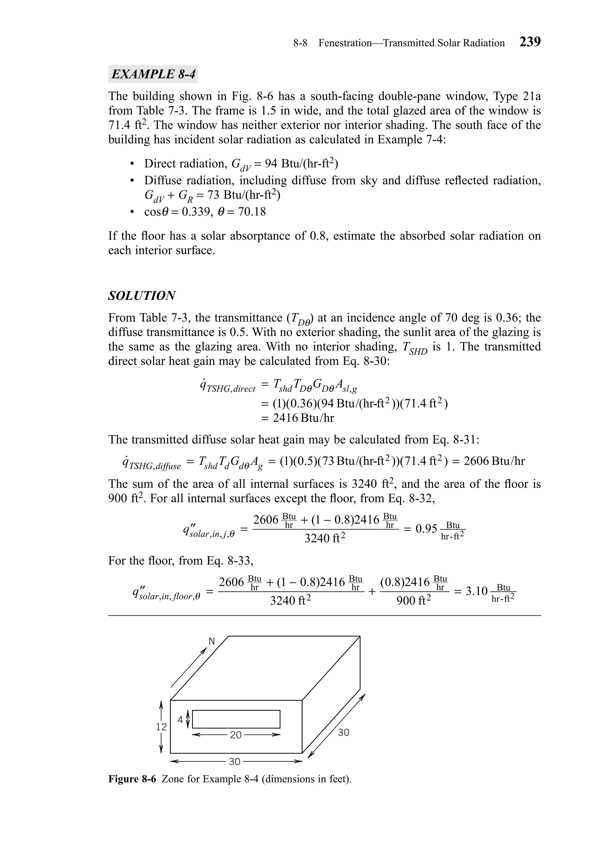
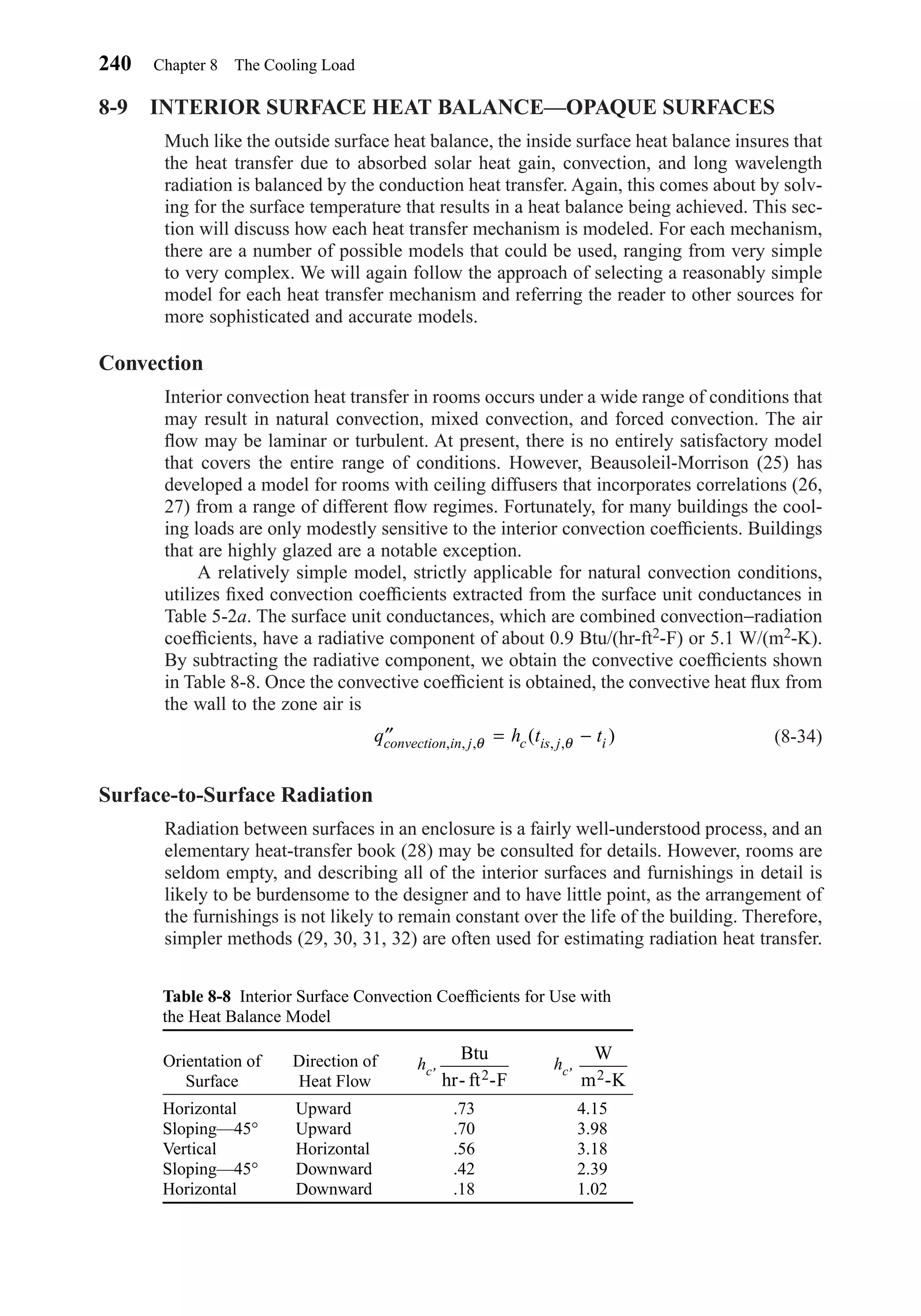
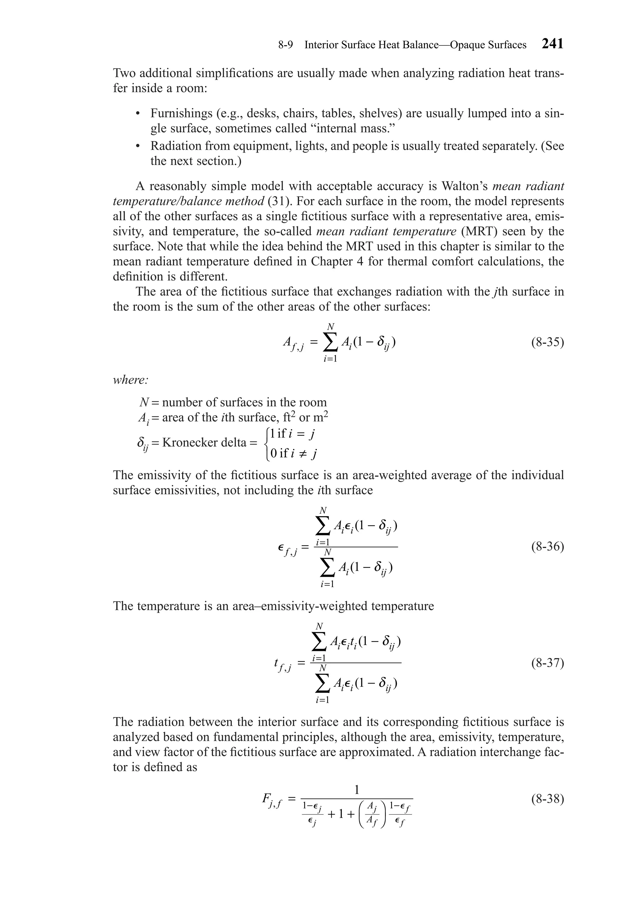
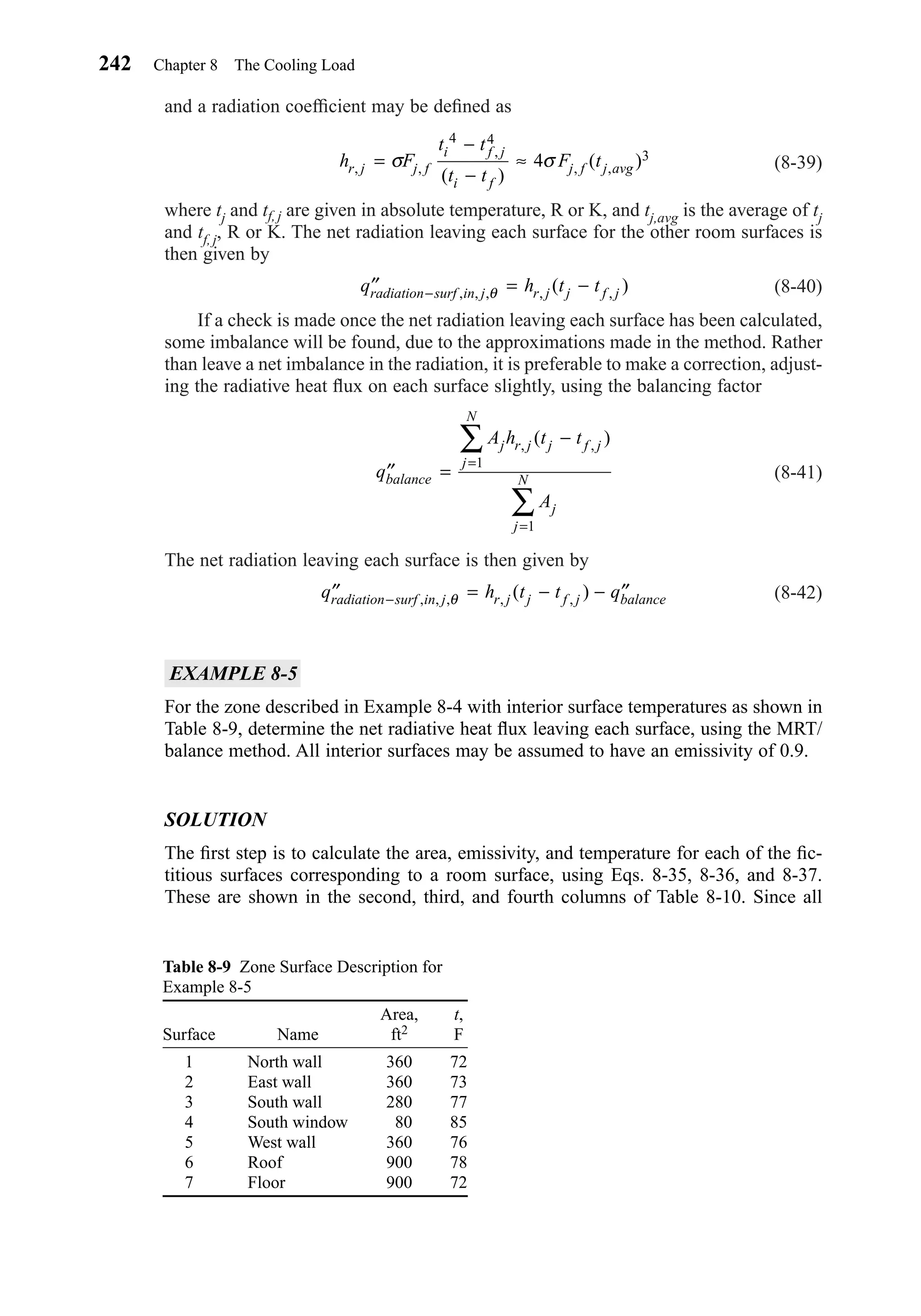
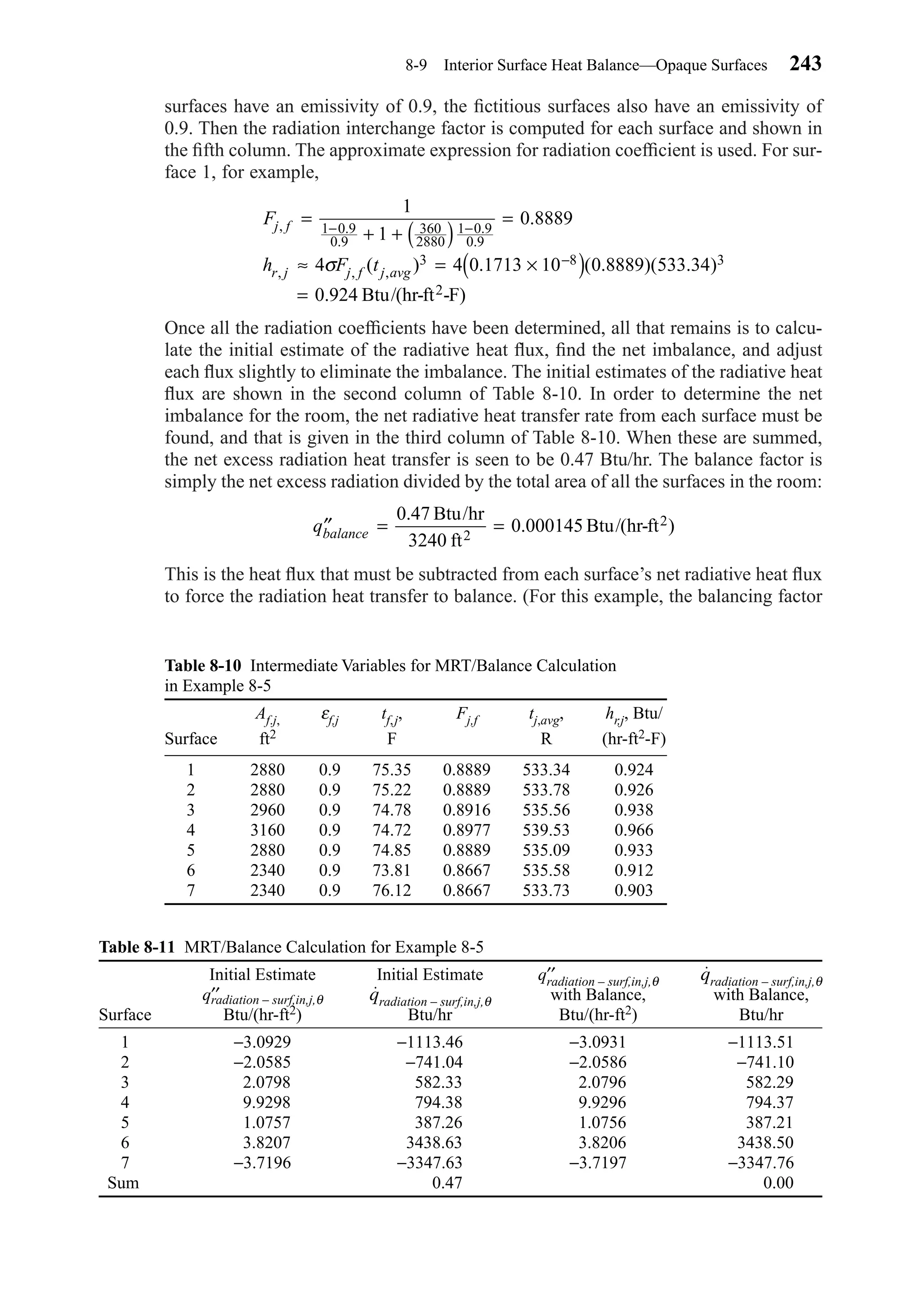
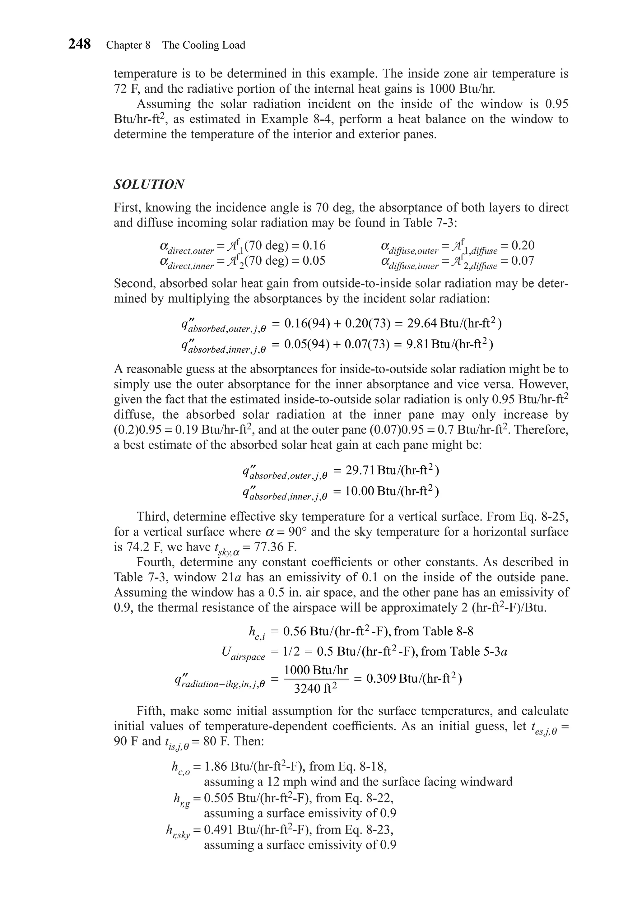
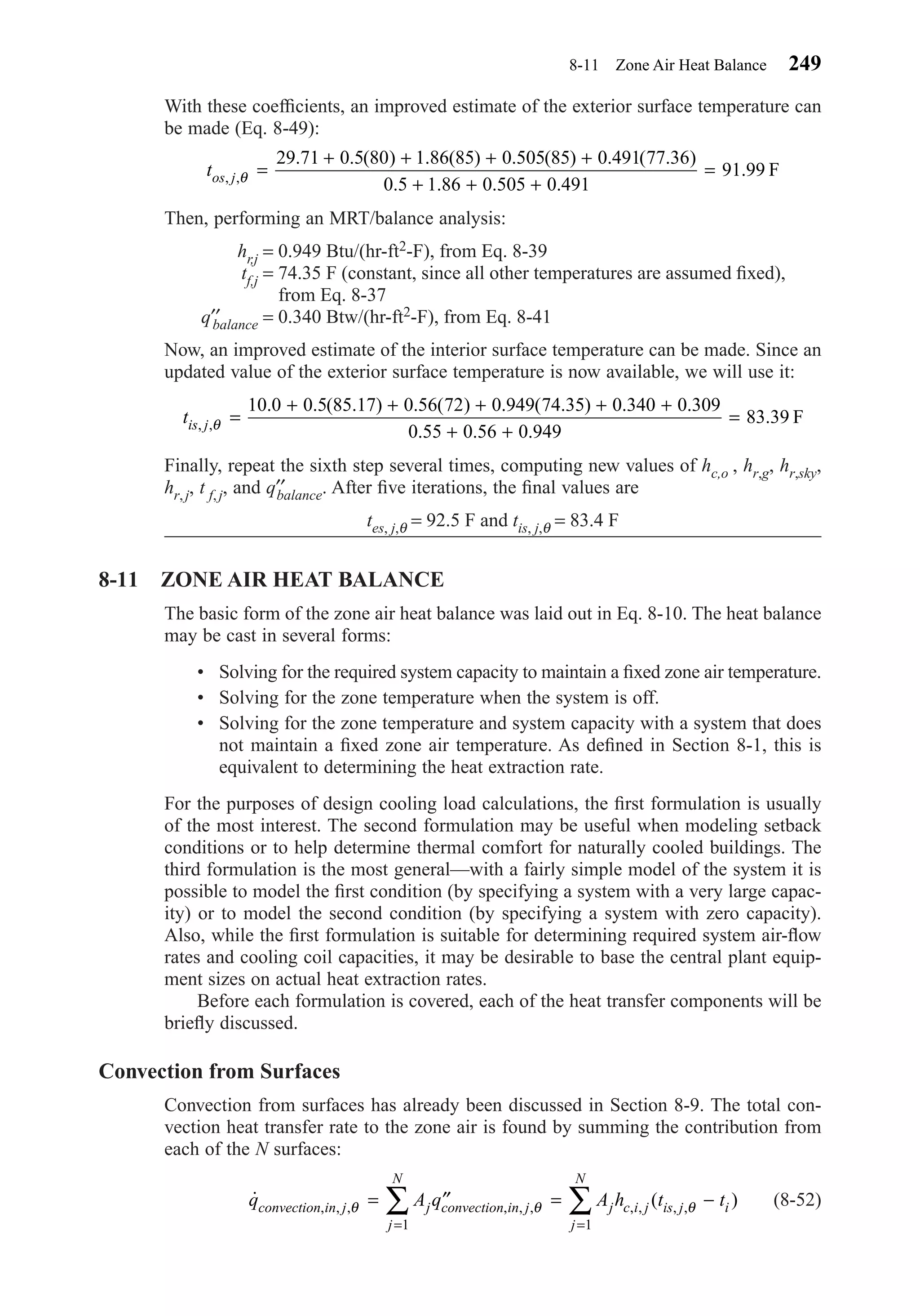
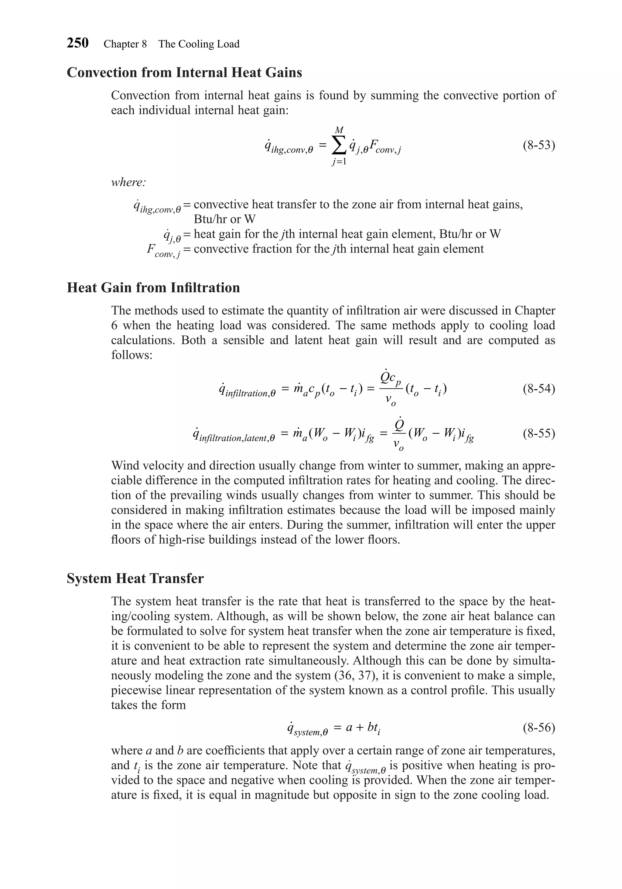
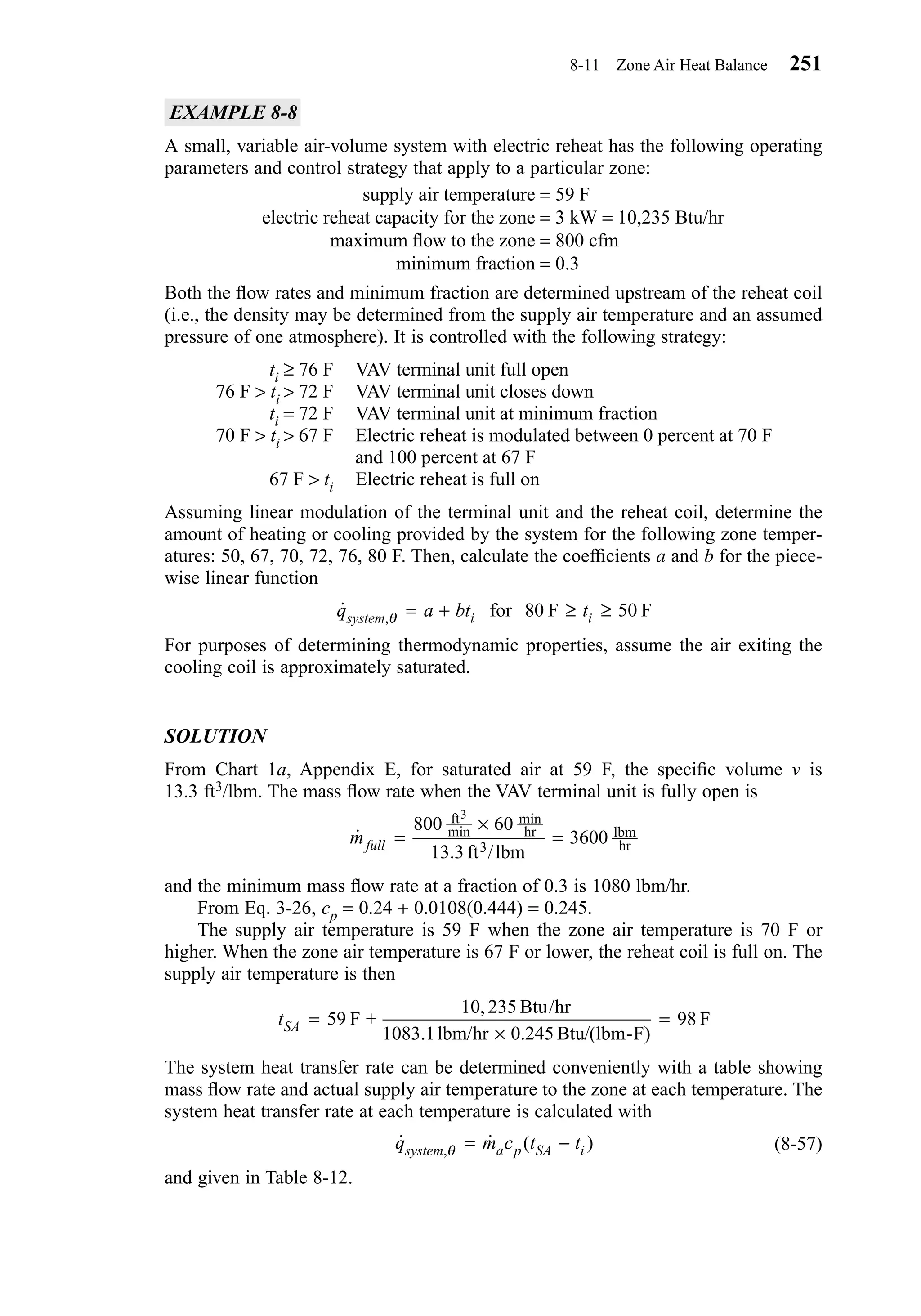
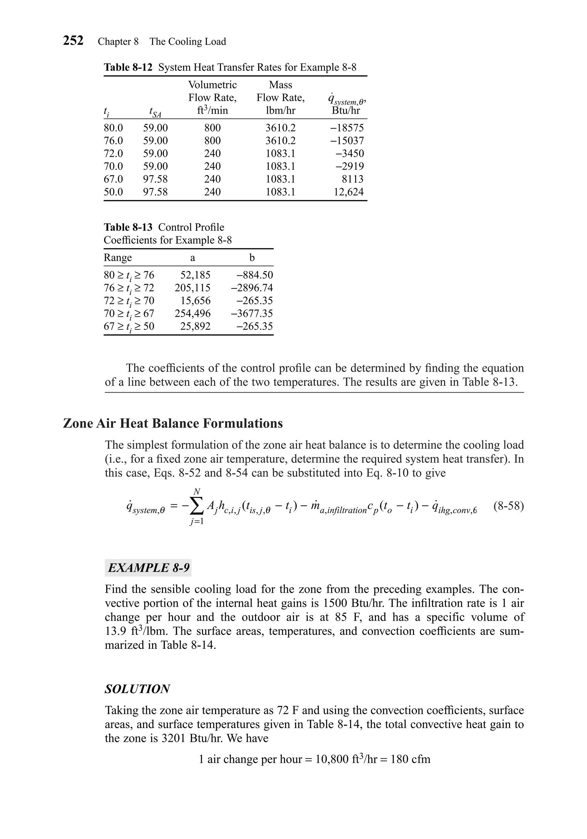
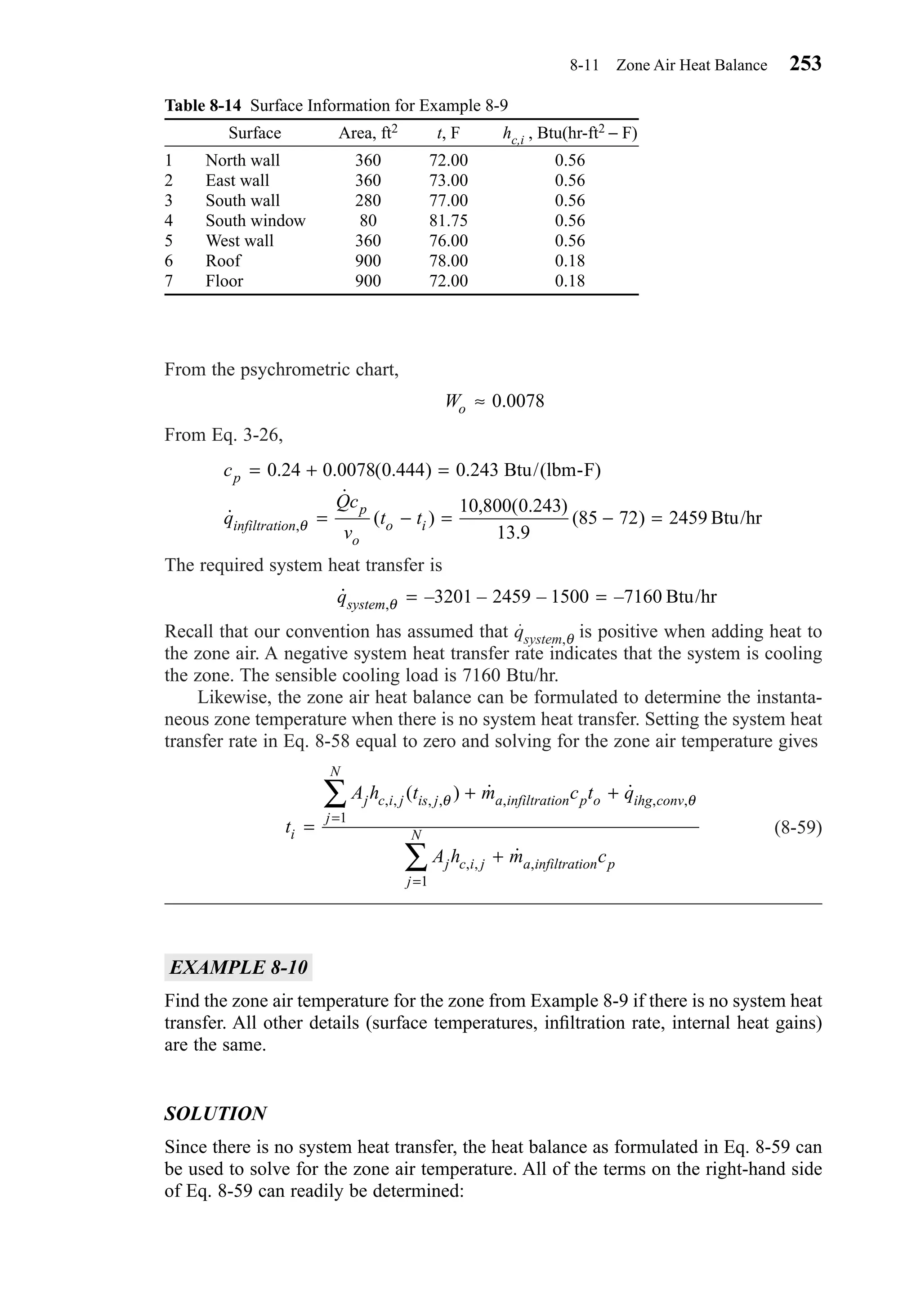
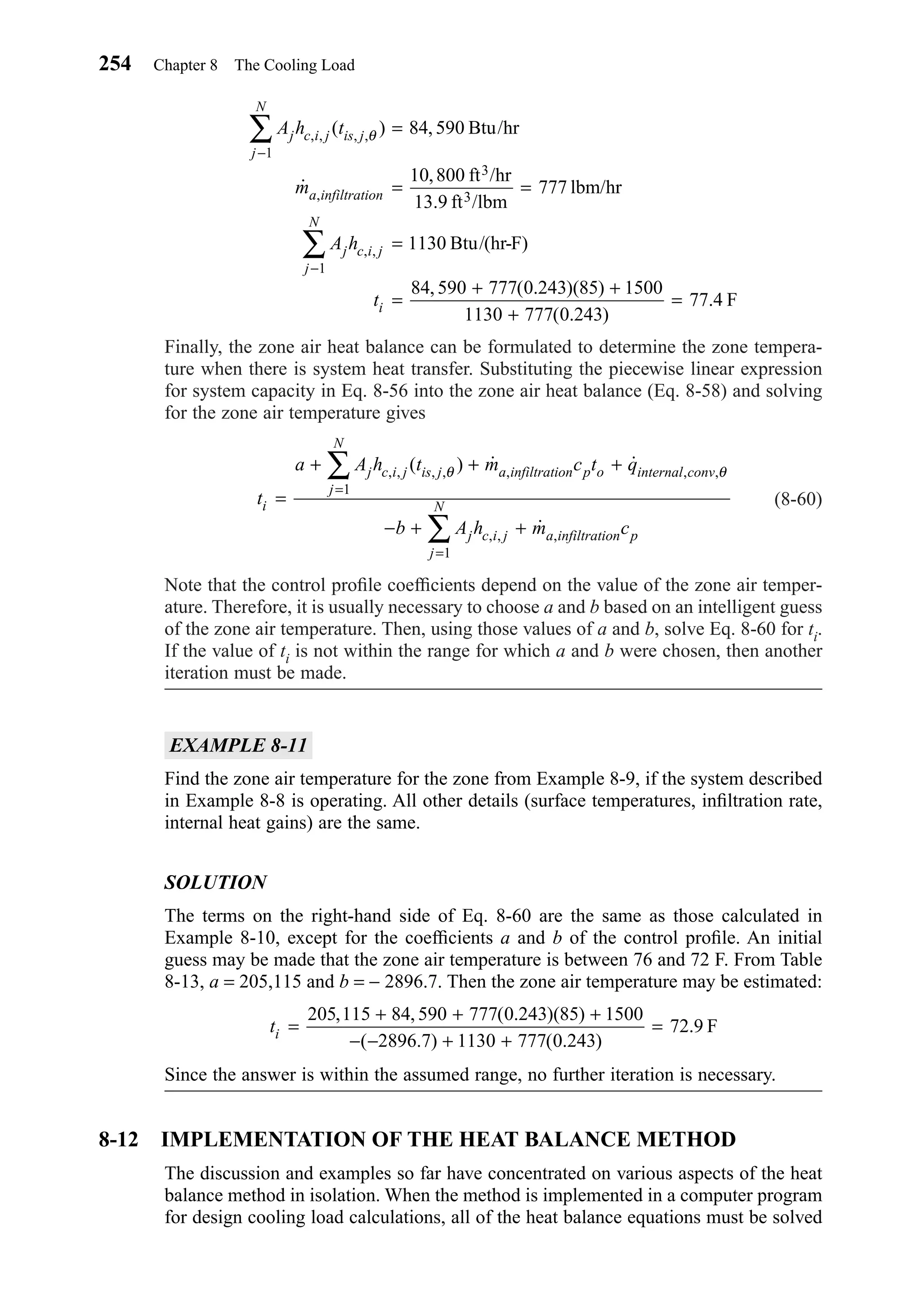
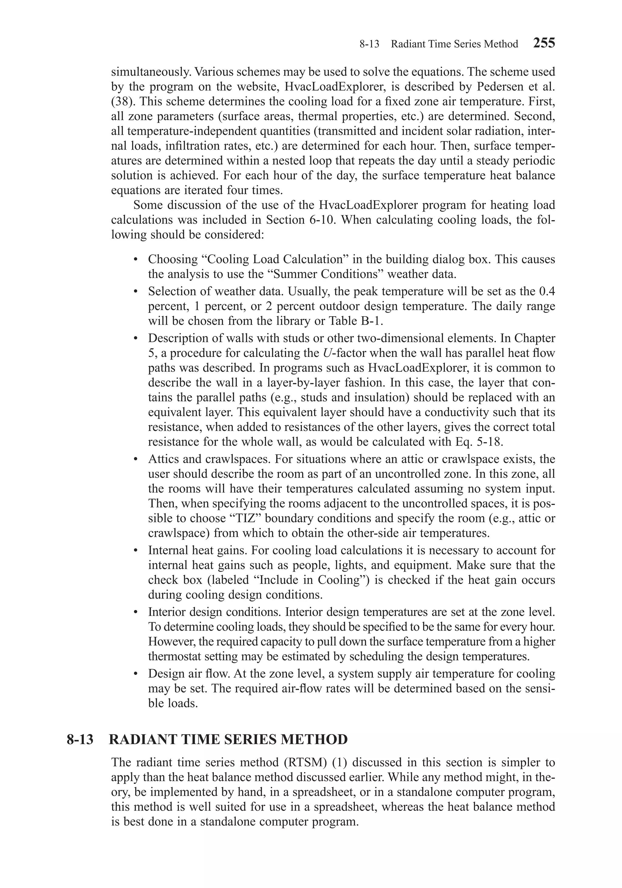
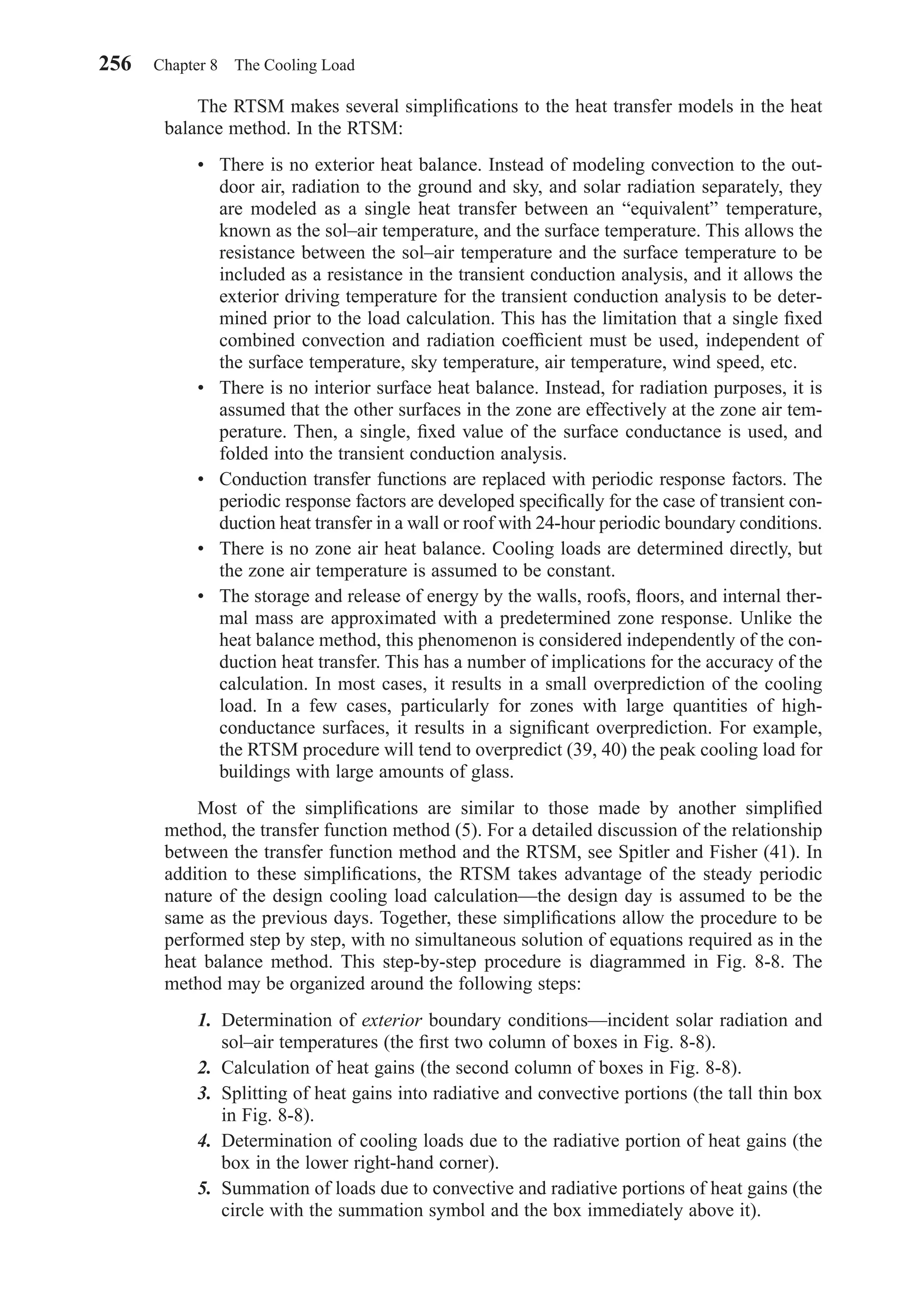

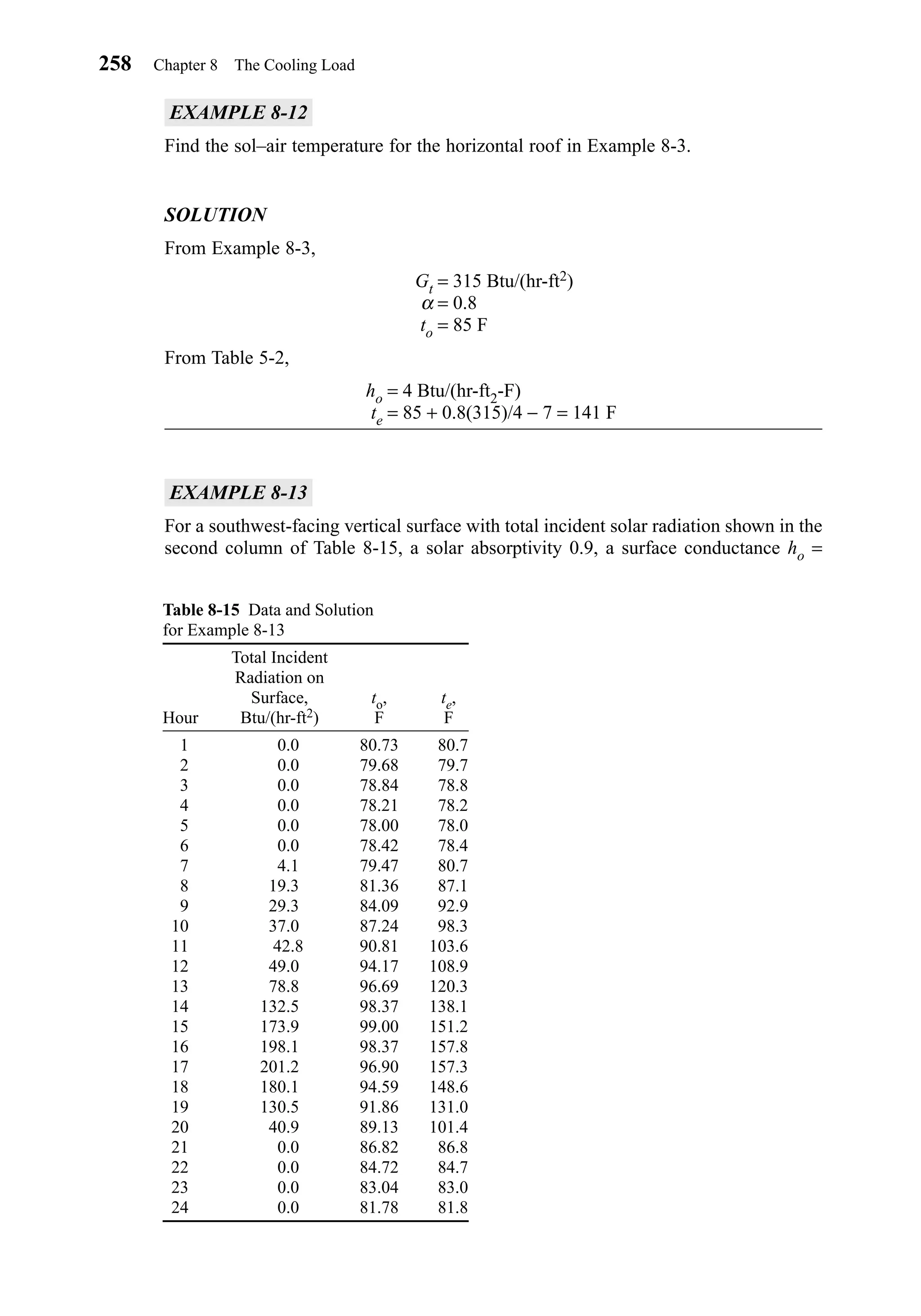
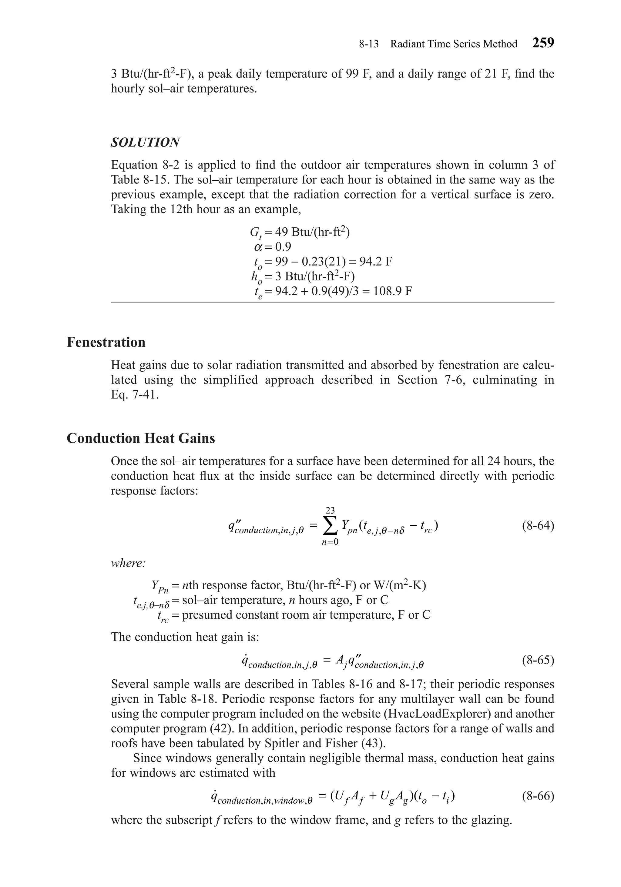

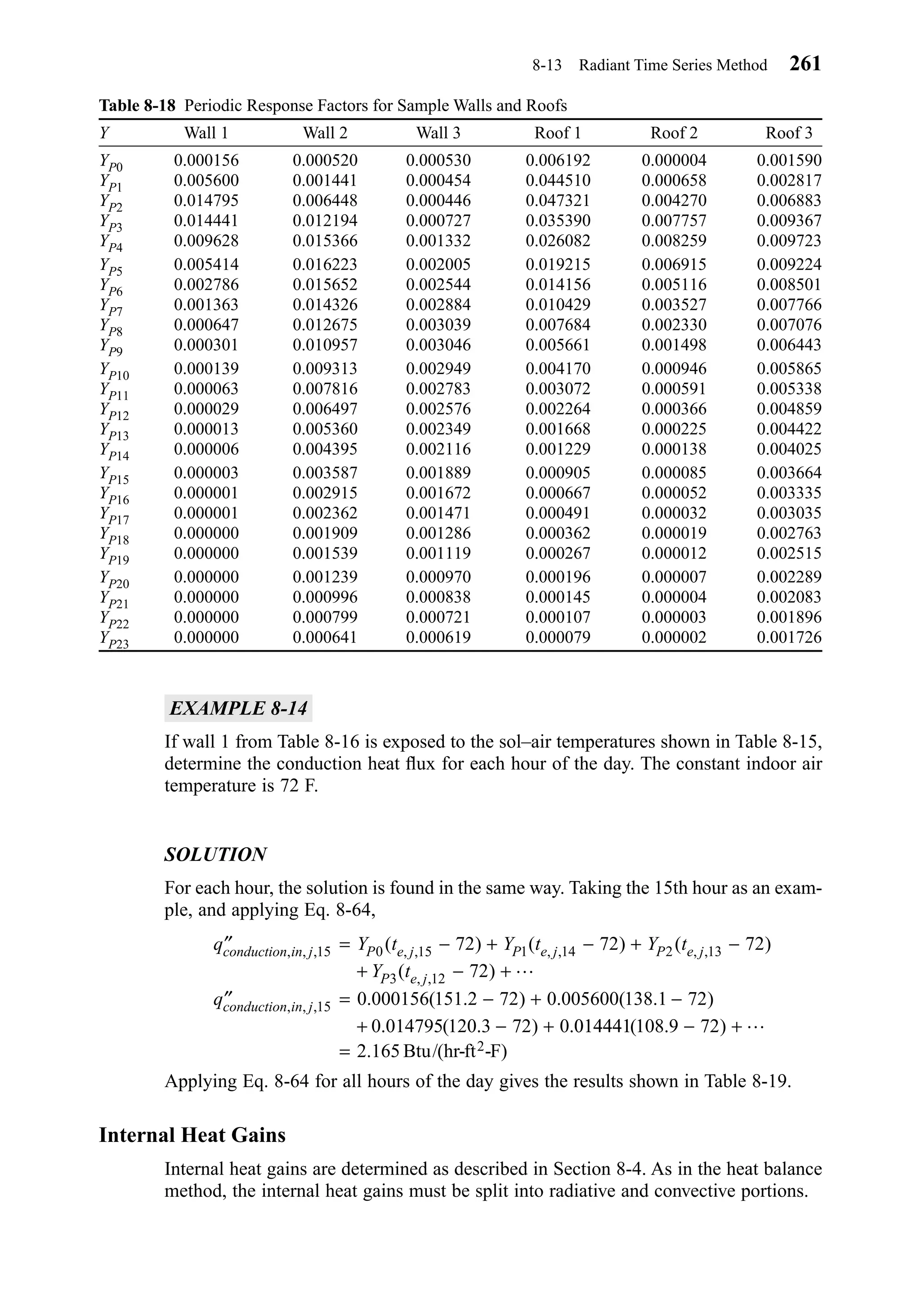
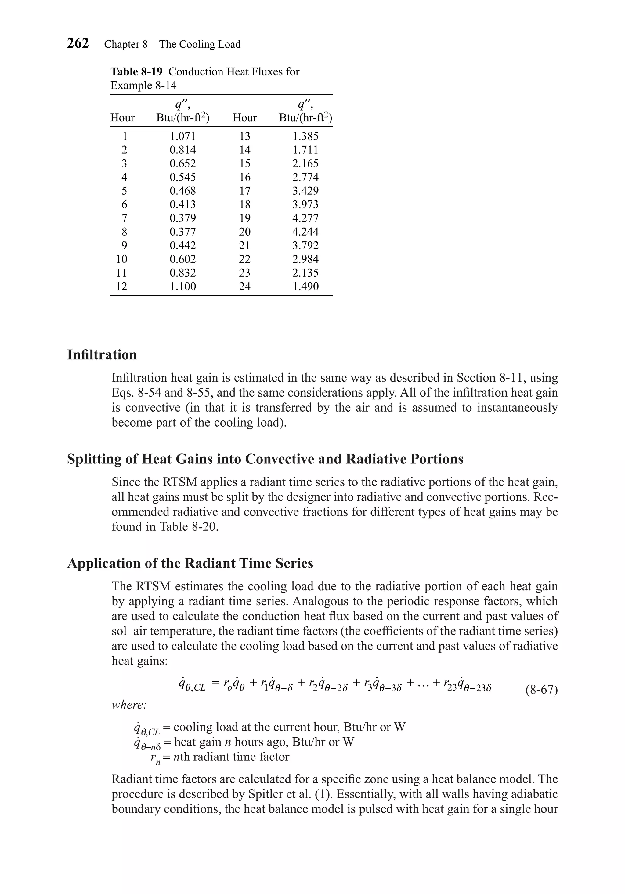
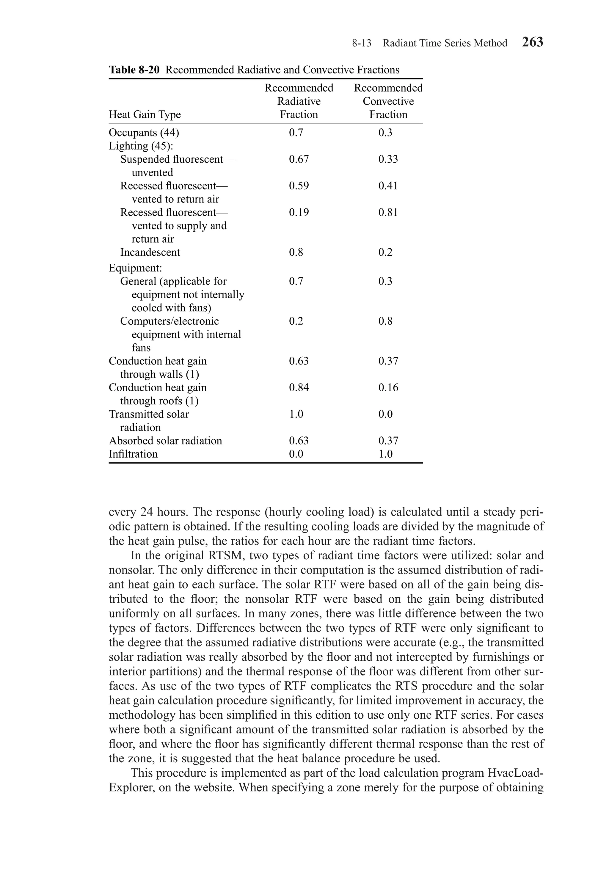
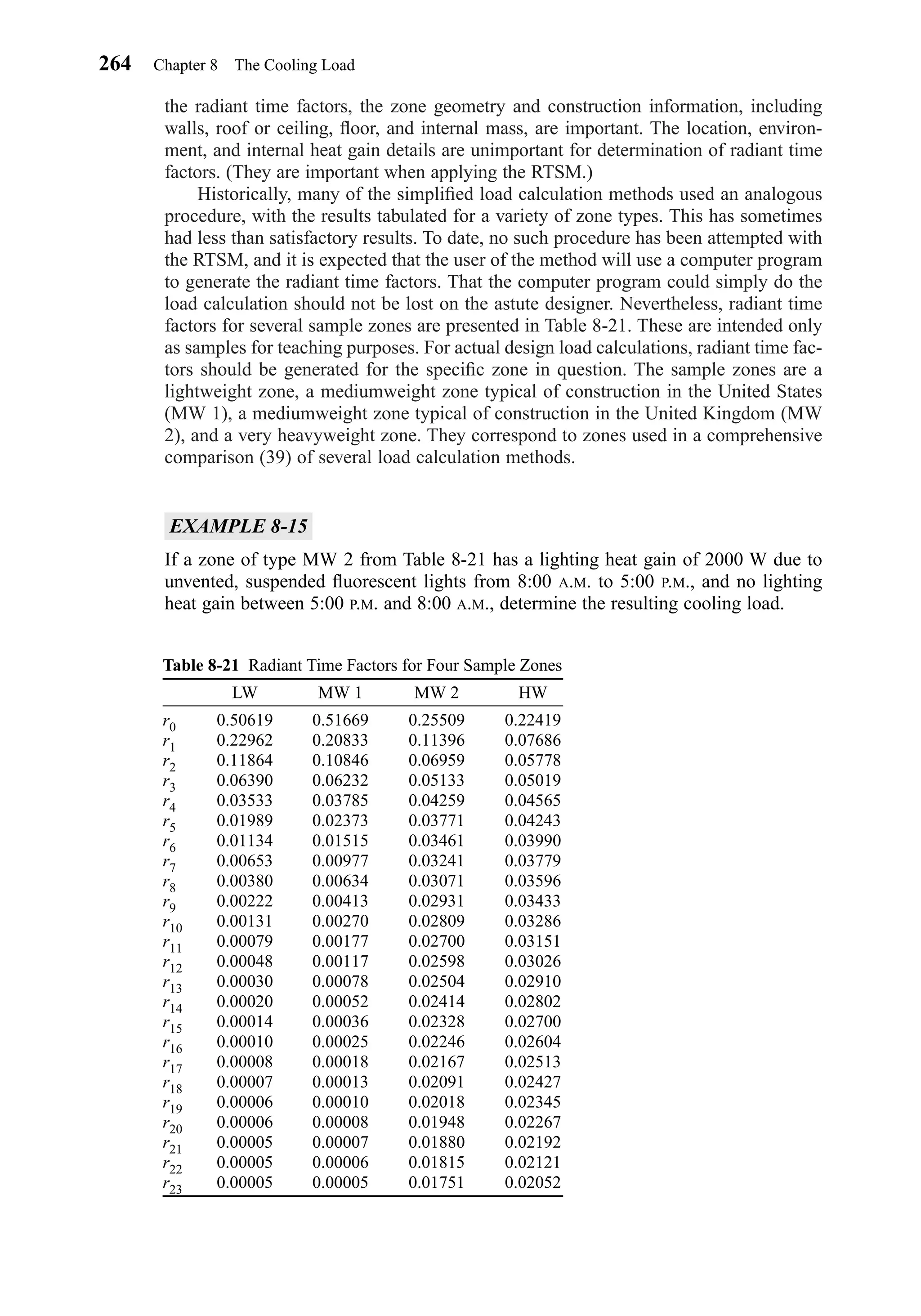
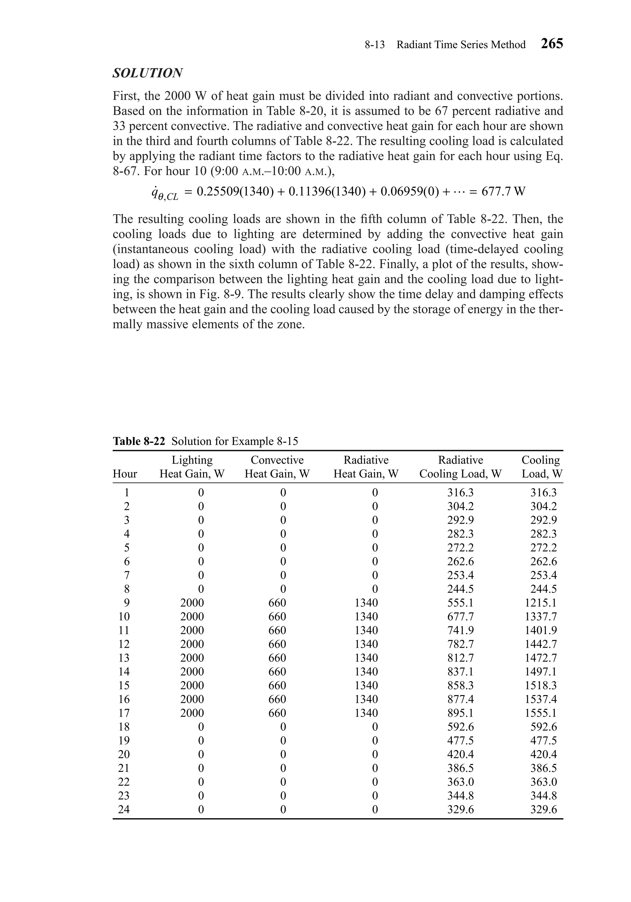
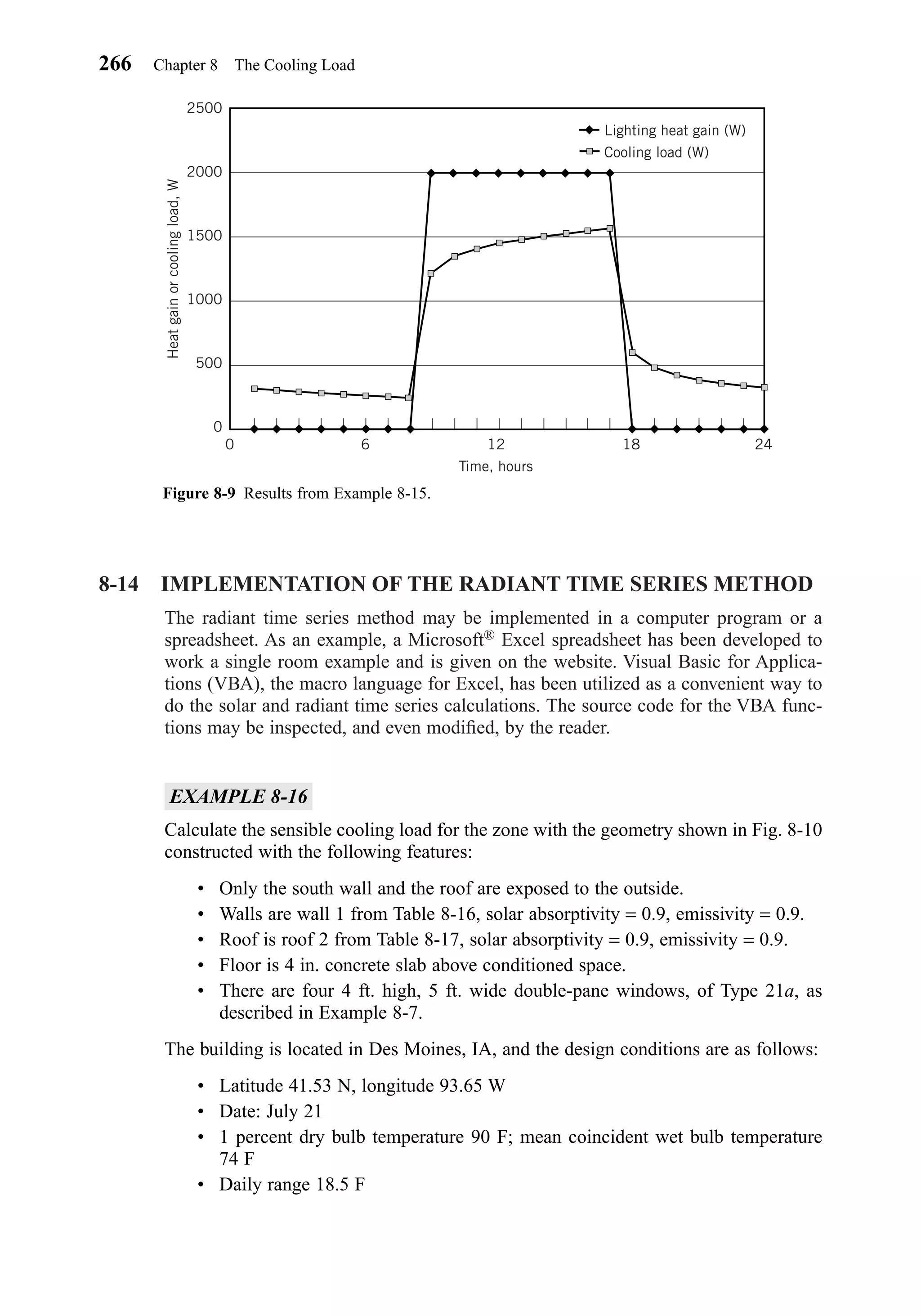
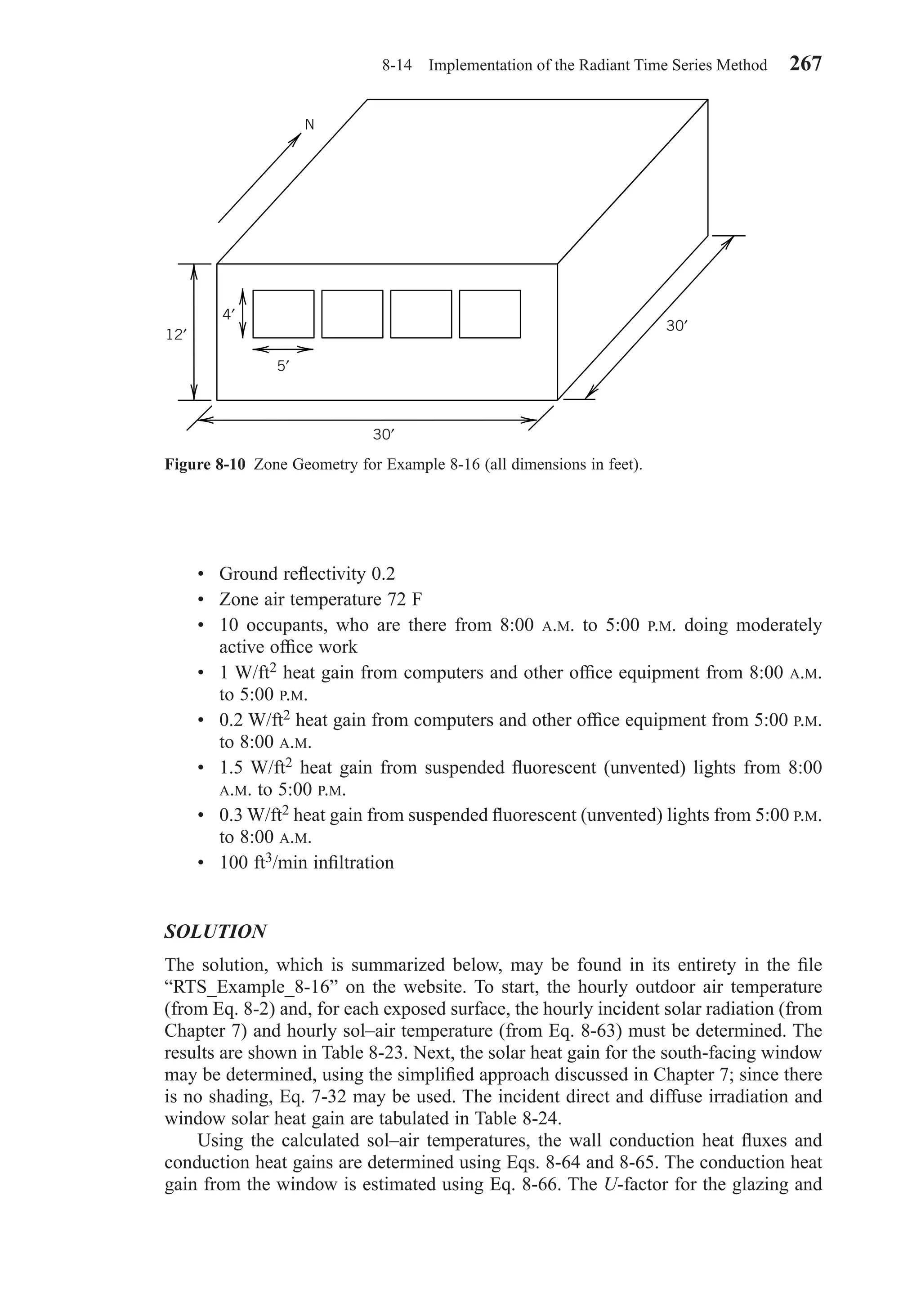
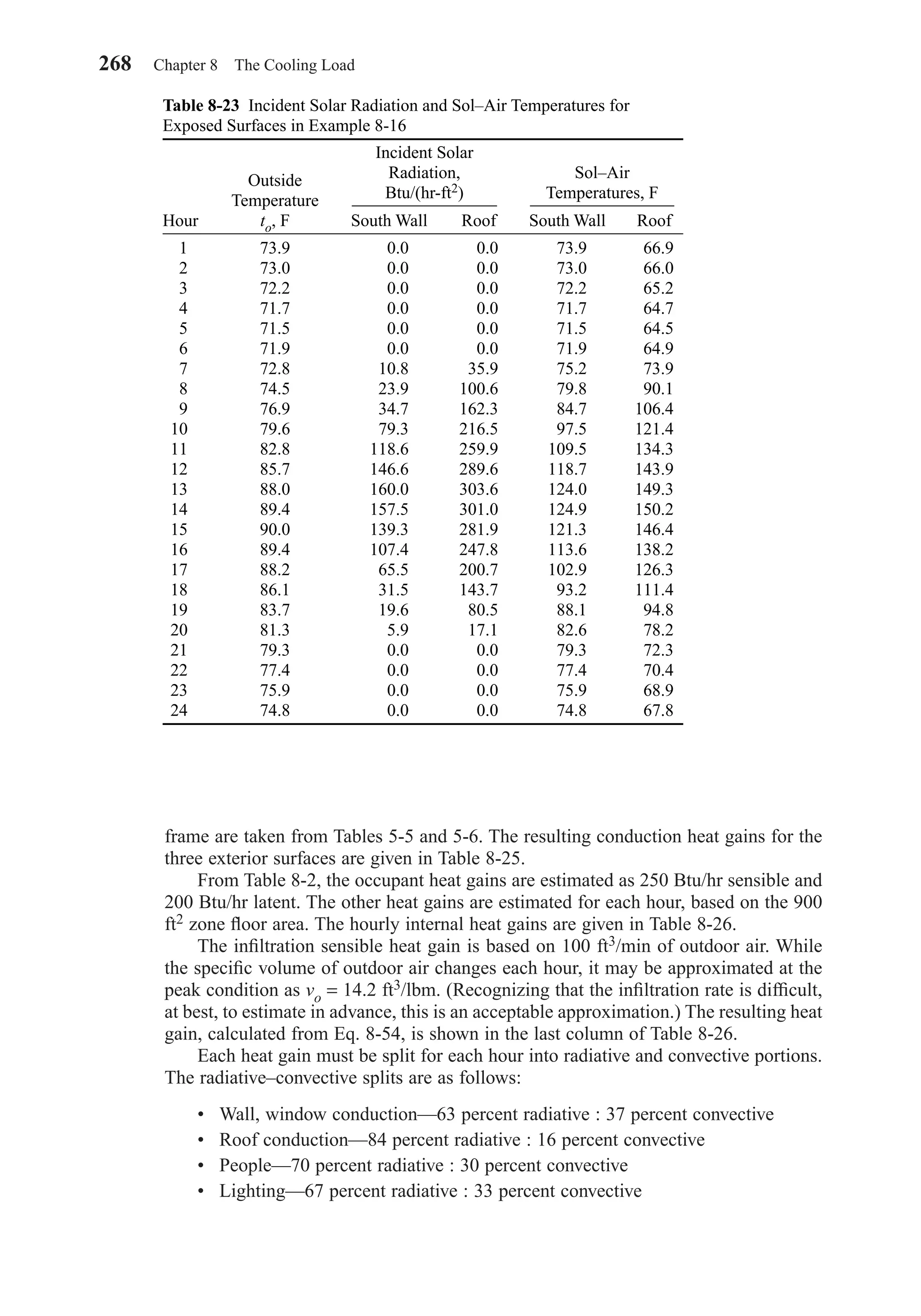
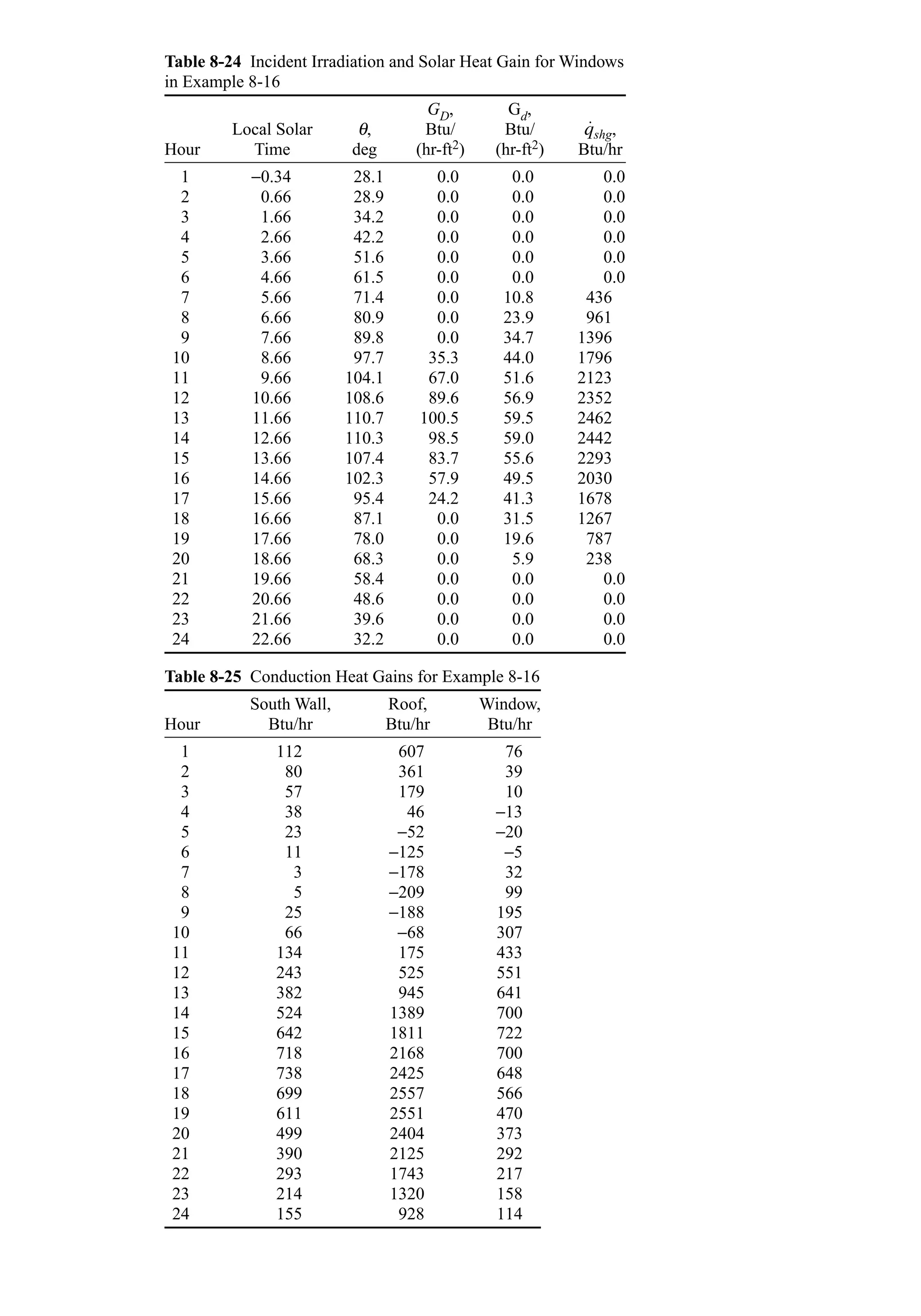
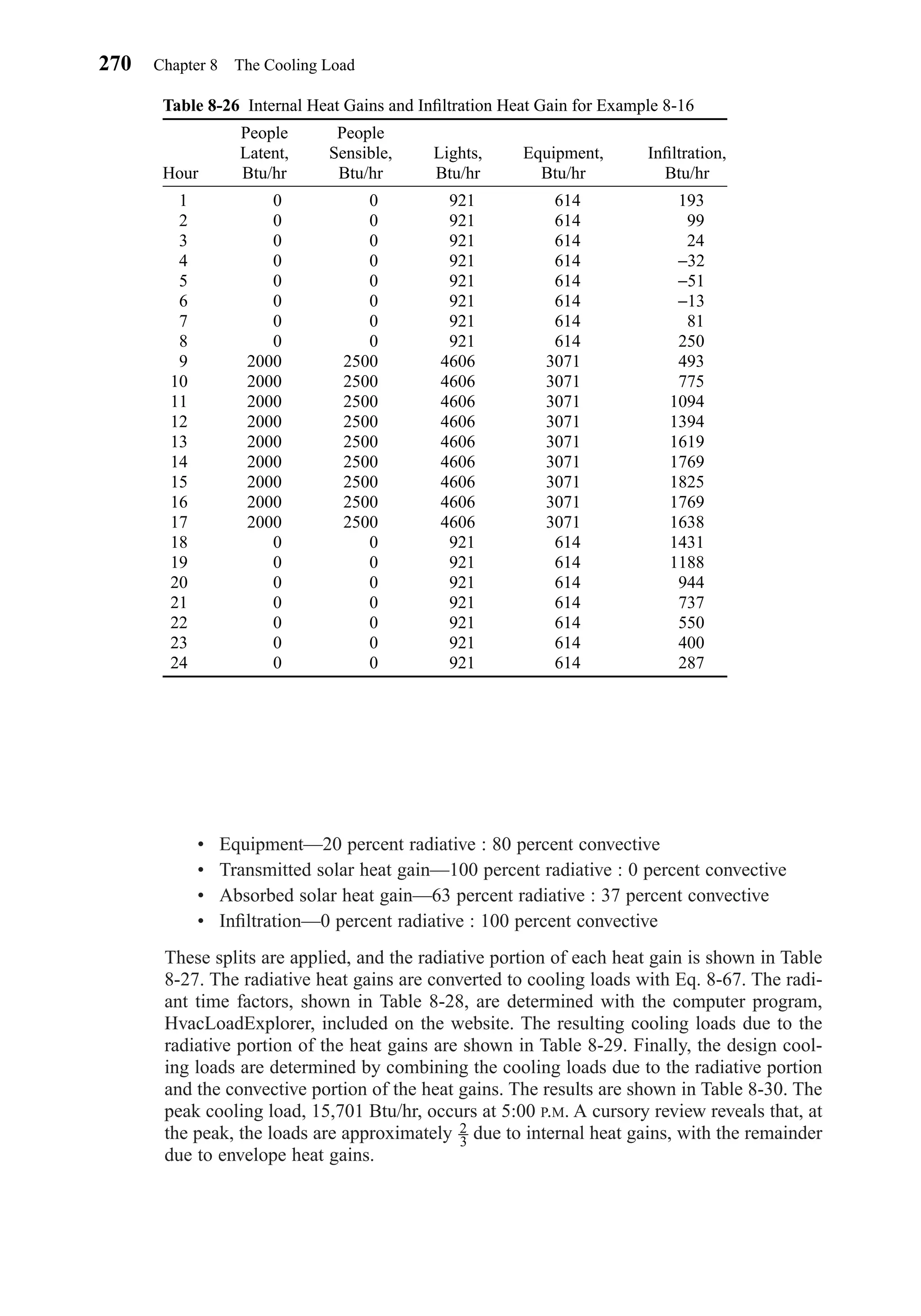

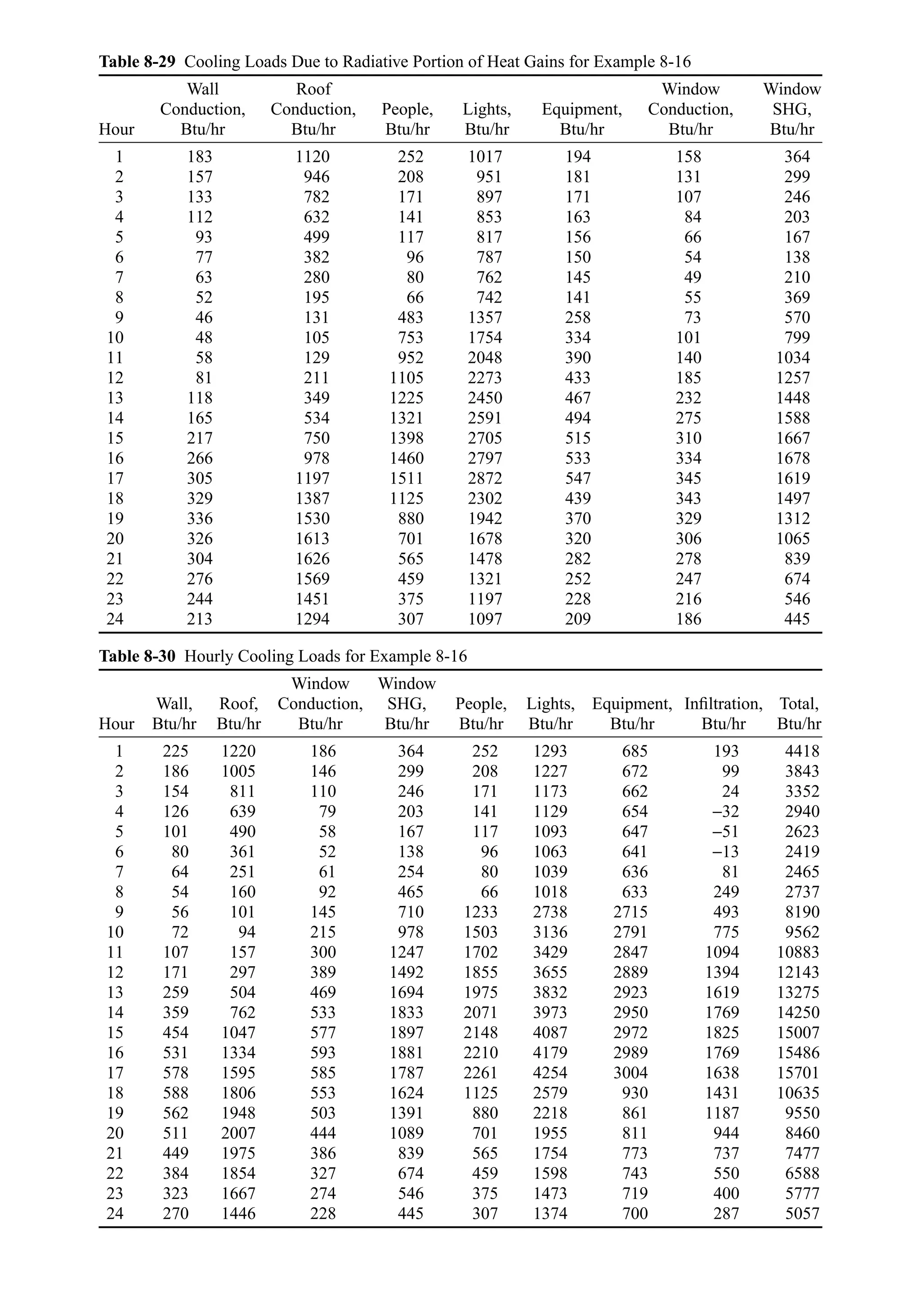
![39. S. J. Rees, J. D. Spitler, and P. Haves, “Quantitative Comparison of North American and U.K. Cool-
ing Load Calculation Procedures—Results,” ASHRAE Transactions, Vol. 104, No. 2, pp. 47–61, 1998.
40. I. S. Iu, D. E. Fisher, C. Chantrasrisalai, and D. Eldridge, “Experimental Validation of Design Cooling
Load Procedures: The Radiant Time Series Method,” ASHRAE Transactions, Vol. 109, No. 2, 2003.
41. J. D. Spitler and D. E. Fisher, “On the Relationship Between the Radiant Time Series and Transfer
Function Methods for Design Cooling Load Calculations,” International Journal of Heating, Venti-
lating, Air-Conditioning and Refrigerating Research, Vol. 5, No. 2, pp. 125–138, 1999.
42. PRF/RTF Generator program. Available from http://www.hvac.okstate.edu, in the Resources section.
43. J. D. Spitler and D. E. Fisher, “Development of Periodic Response Factors for Use with the Radiant
Time Series Method,” ASHRAE Transactions, Vol. 105, No. 2, pp. 491–509, 1999.
PROBLEMS
8-1. Describe a situation where the heat gain to the space is (a) greater than the cooling load at a
given time, (b) less than the cooling load at a given time, and (c) equal to the cooling load at
a given time.
8-2. Southern coastal regions of the United States experience periods of very high humidity. Explain
how this might influence selection of design conditions.
8-3. Determine the ASHRAE Standard 90.1 design conditions for the following locations. Include
the maximum outdoor temperature, the outdoor mean coincident wet bulb temperature, the
indoor dry bulb temperature, the relative humidity, the elevation, and the latitude. (a) Norfolk,
VA, (b) Pendleton, OR, (c) Casper, WY, and (d) Shreveport, LA.
8-4. Determine the wall conduction transfer function coefficients for a wall composed of 4 in. brick
[k = 7 (Btu-in.)/(hr-ft2-F)], in. regular density sheathing (vegetable fiber board), in. min-
eral fiber insulation (R-13), and in. gypsum board.
8-5. Change the insulation in Problem 8-4 to R-19, and determine the conduction transfer function
coefficients.
8-6. A roof is composed of asphalt roll roofing, in. plywood, in. mineral fiber insulation (R-19),
and in. gypsum board. Determine the conduction transfer function coefficients.
8-7. The roof of Problem 8-6 is changed to have a suspended ceiling with a 12 in. air space above
it. Determine the conduction transfer function coefficients.
8-8. A roof is composed of asphalt roll roofing, 4 in. of 120 lb/ft3 limestone concrete, 2 in. of
expanded polystyrene, a in. airspace, and 0.5 in. of acoustical tile. Determine the conduc-
tion transfer function coefficients.
8-9. A wall has an incident solar radiation of 300 Btu/(hr-ft2), an outside air temperature of 98 F, and
an outside wind speed of 15 mph. The wall has a solar absorptivity of 0.6, a thermal emissivity of
0.9, negligible thermal mass, an outside-surface-to-inside-surface U-factor of 0.1 Btu/(hr-ft2-F),
and an inside surface temperature of 72 F. Determine the conduction heat flux.
8-10. Compute the solar irradiation for a west-facing wall in Albuquerque, NM, for each hour of the
day on July 21. Assume 0.4 percent outdoor design conditions. The wall has a solar absorptiv-
ity of 0.8, a thermal emissivity of 0.9, negligible thermal mass, an outside-surface-to-inside-
surface U-factor of 0.1 Btu/(hr-ft2-F), and an inside surface temperature of 72 F. Determine the
conduction heat flux for each hour.
8-11. Compute the solar irradiation for a south-facing wall in Boise, ID, for each hour of the day on
July 21. Assume 0.4 percent outdoor design conditions. The wall has a solar absorptivity of 0.9,
a thermal emissivity of 0.9, negligible thermal mass, an outside-surface-to-inside-surface
U-factor of 0.1 Btu/(hr-ft2-F), and an inside surface temperature of 72 F. Determine the con-
duction heat flux for each hour.
8-12. For the wall described in Problem 8-4, with an outside surface temperature profile given by
Table 8-5 and a constant inside surface temperature of 70 F, determine the inside conduction
heat flux for each hour.
3 1
2
1
2
5 1
2
1
2
1
2
3 1
2
1
2
Problems 275
Chapter08.qxd 6/15/04 4:06 PM Page 275](https://image.slidesharecdn.com/fayec-160521192803/75/Faye-c-mc_quiston_-_jerald_d-_parker_-_jeffrey_d-293-2048.jpg)
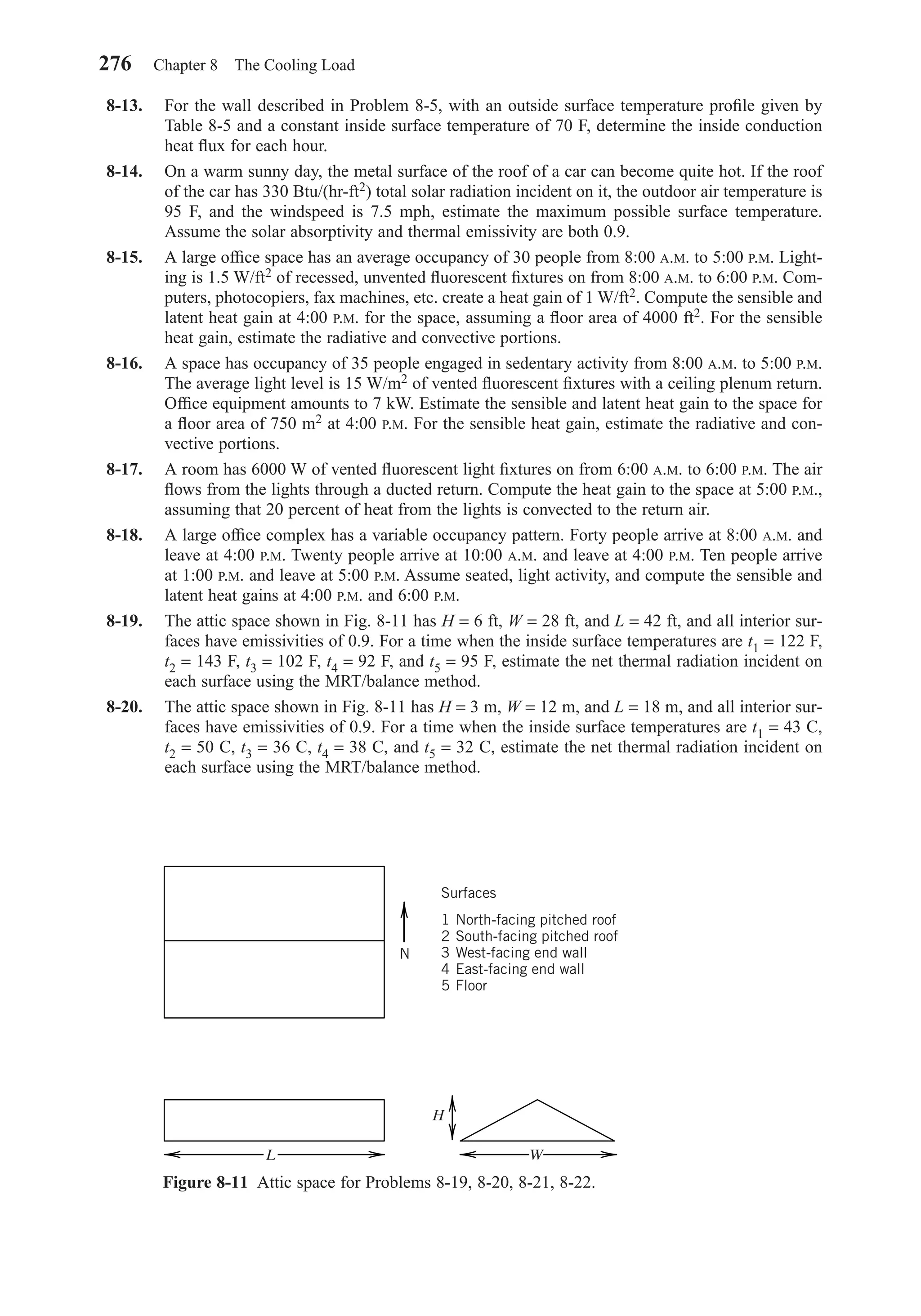
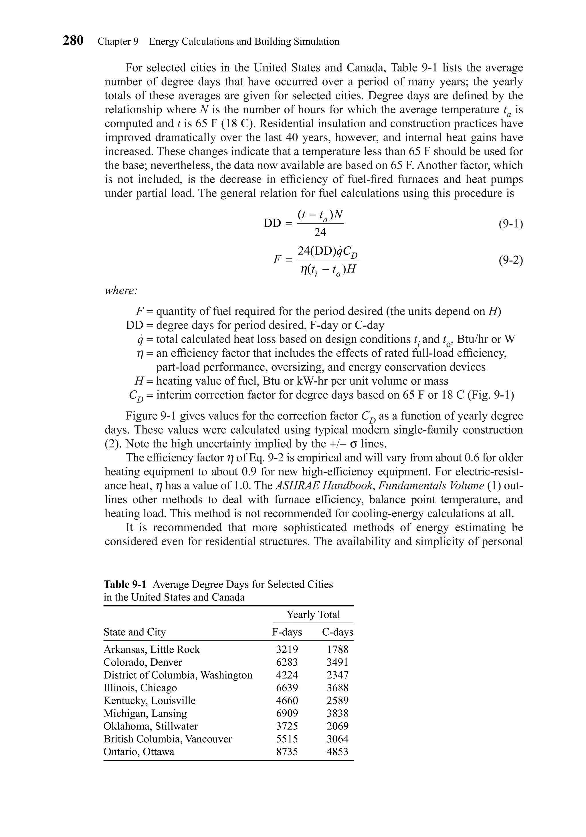
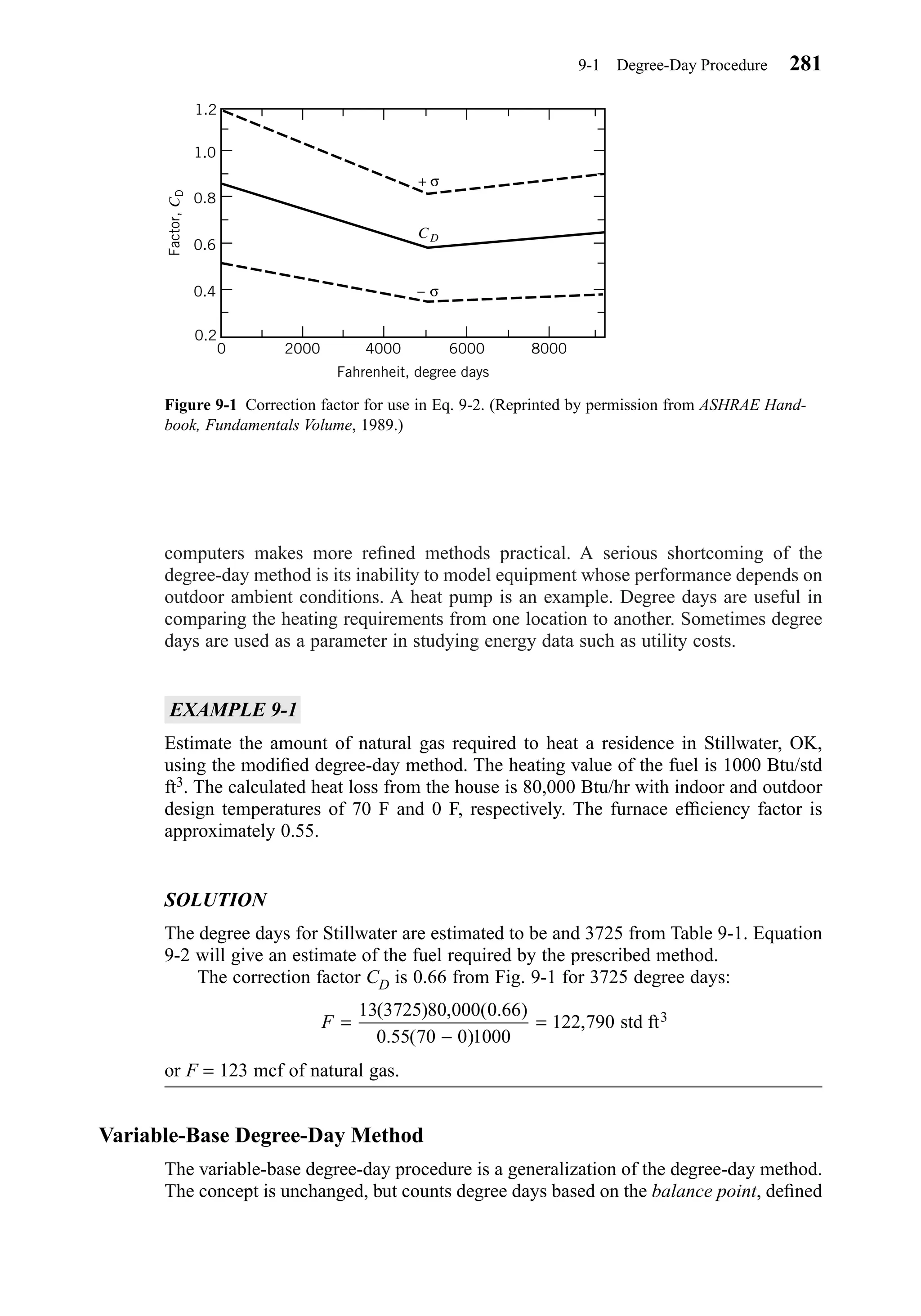

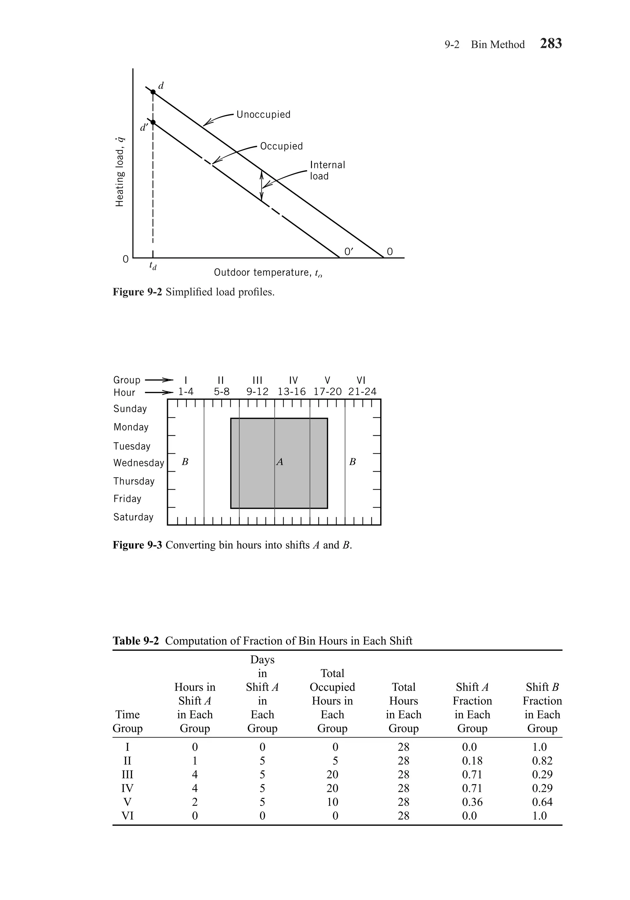
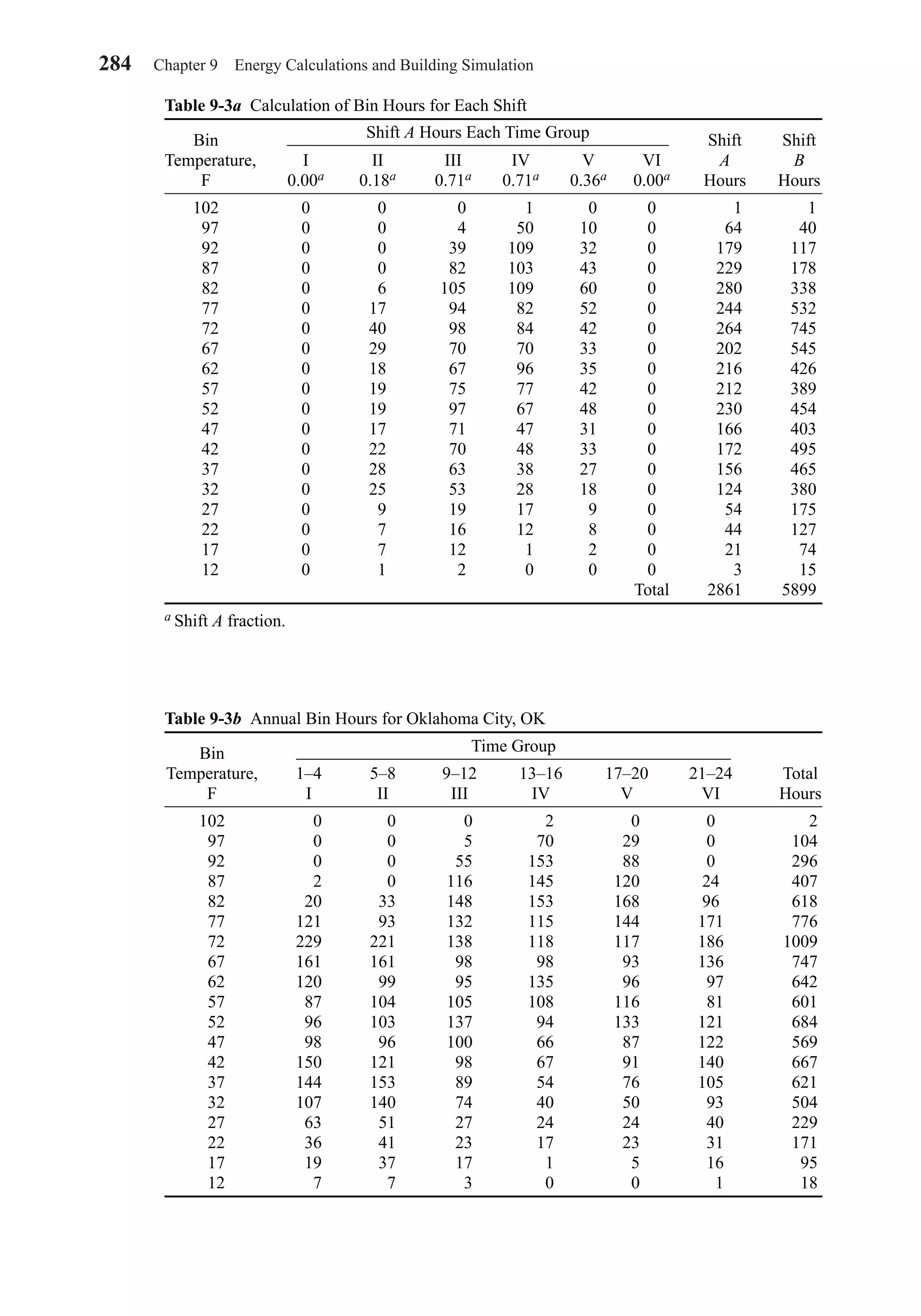
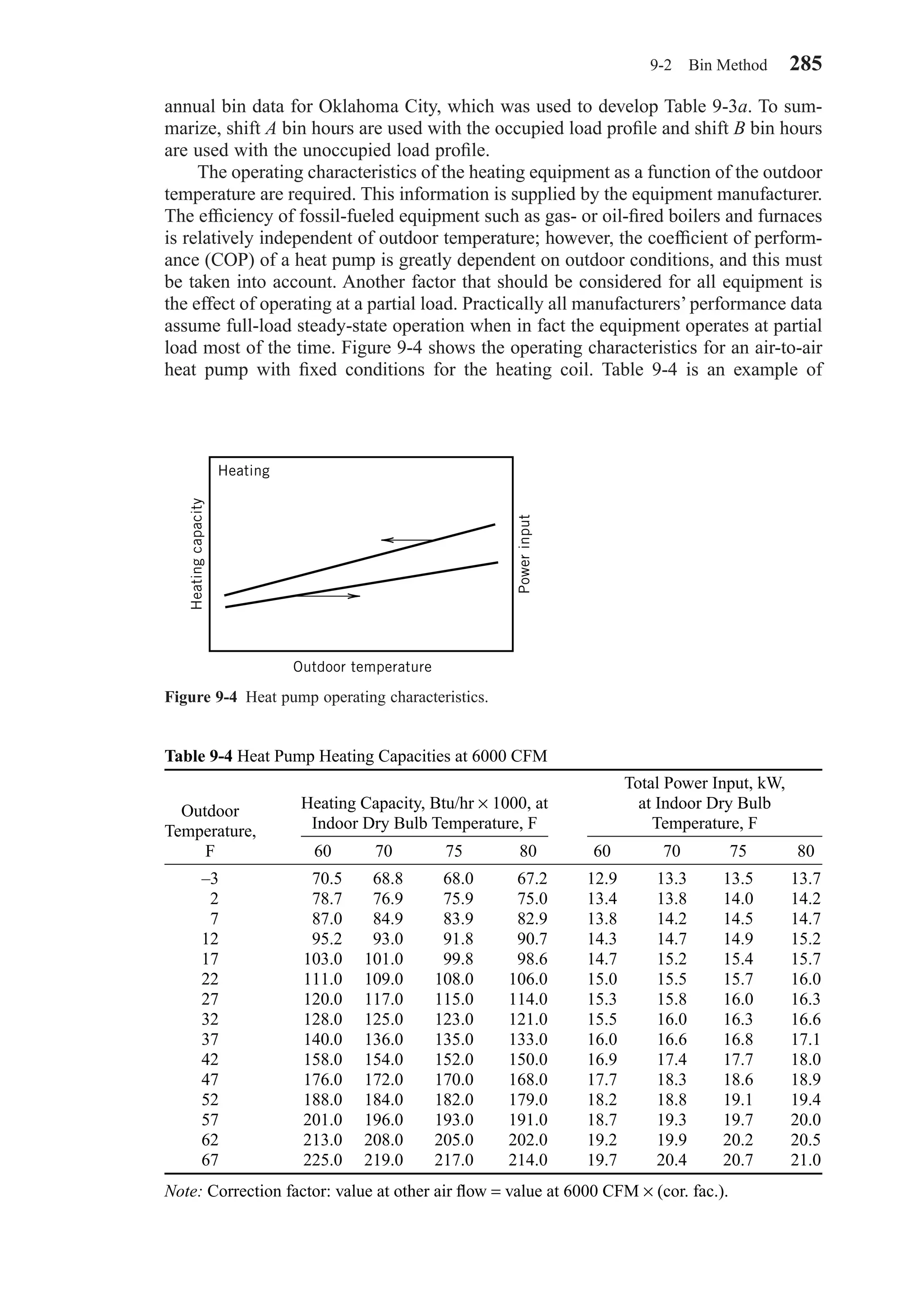
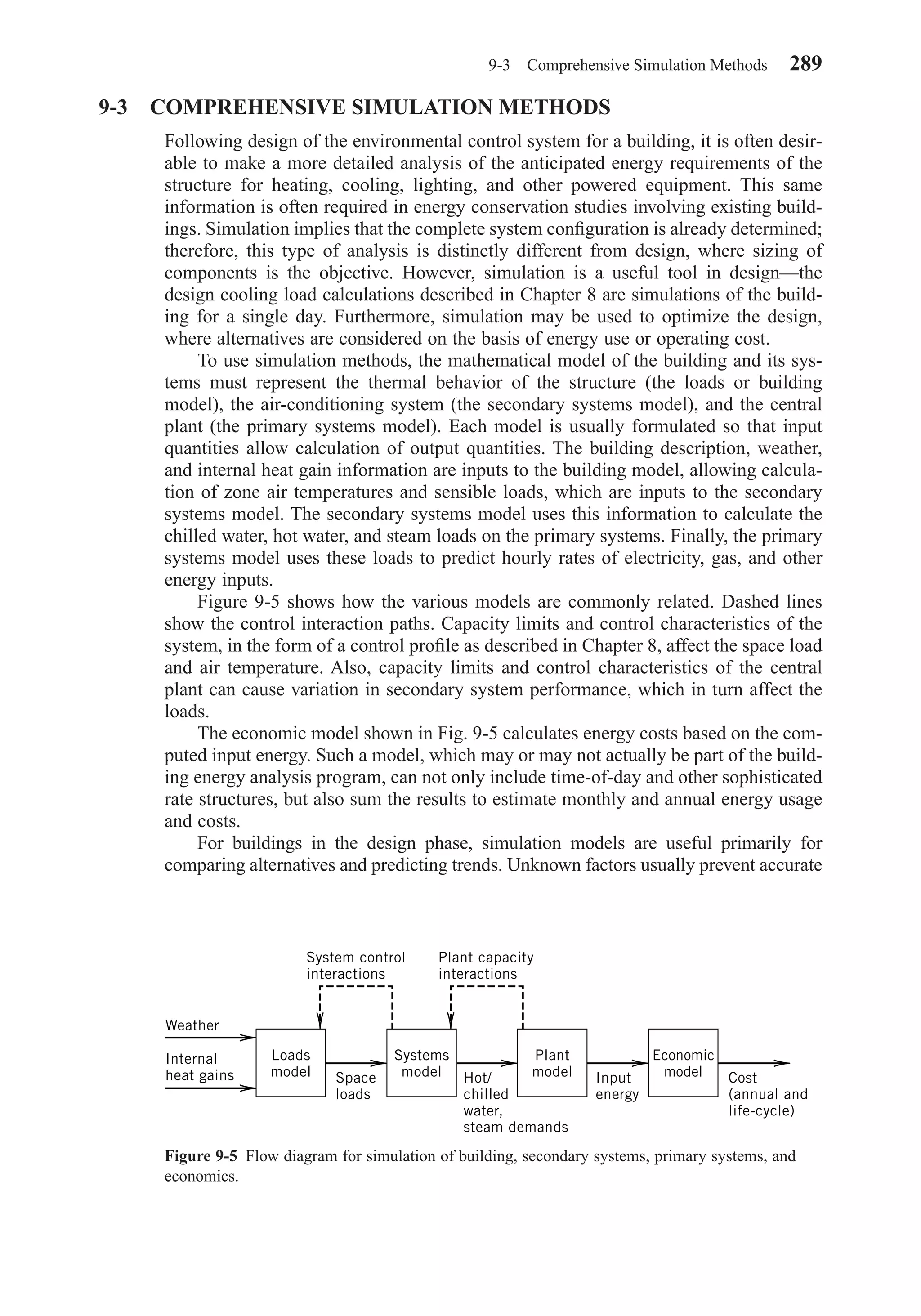

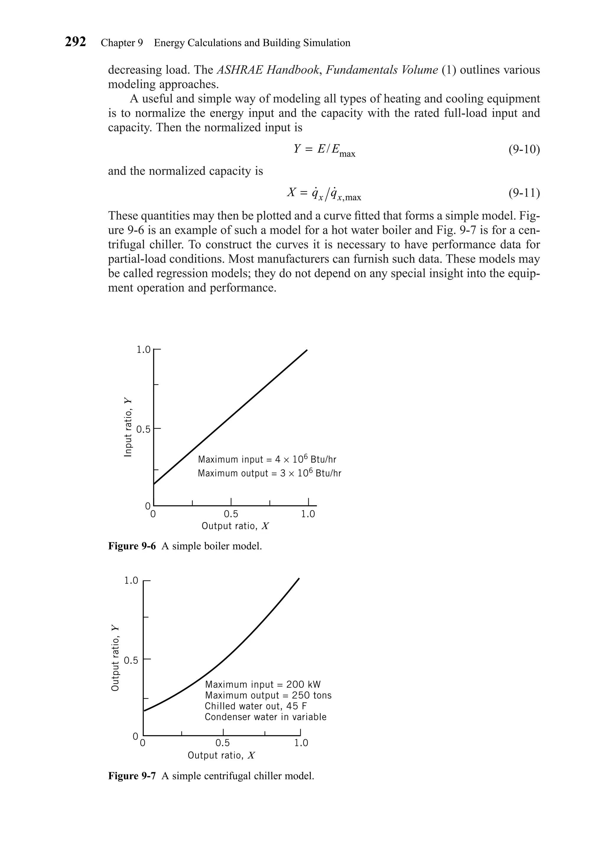
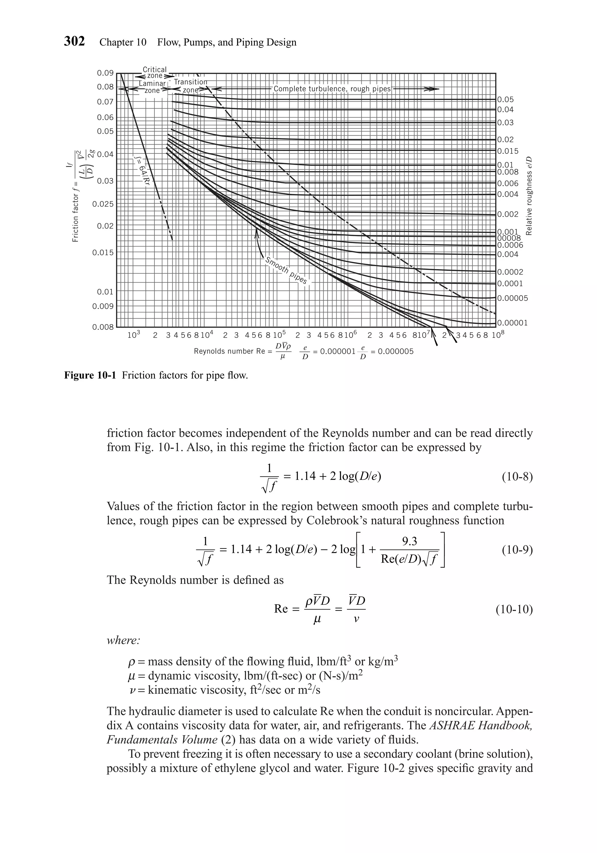
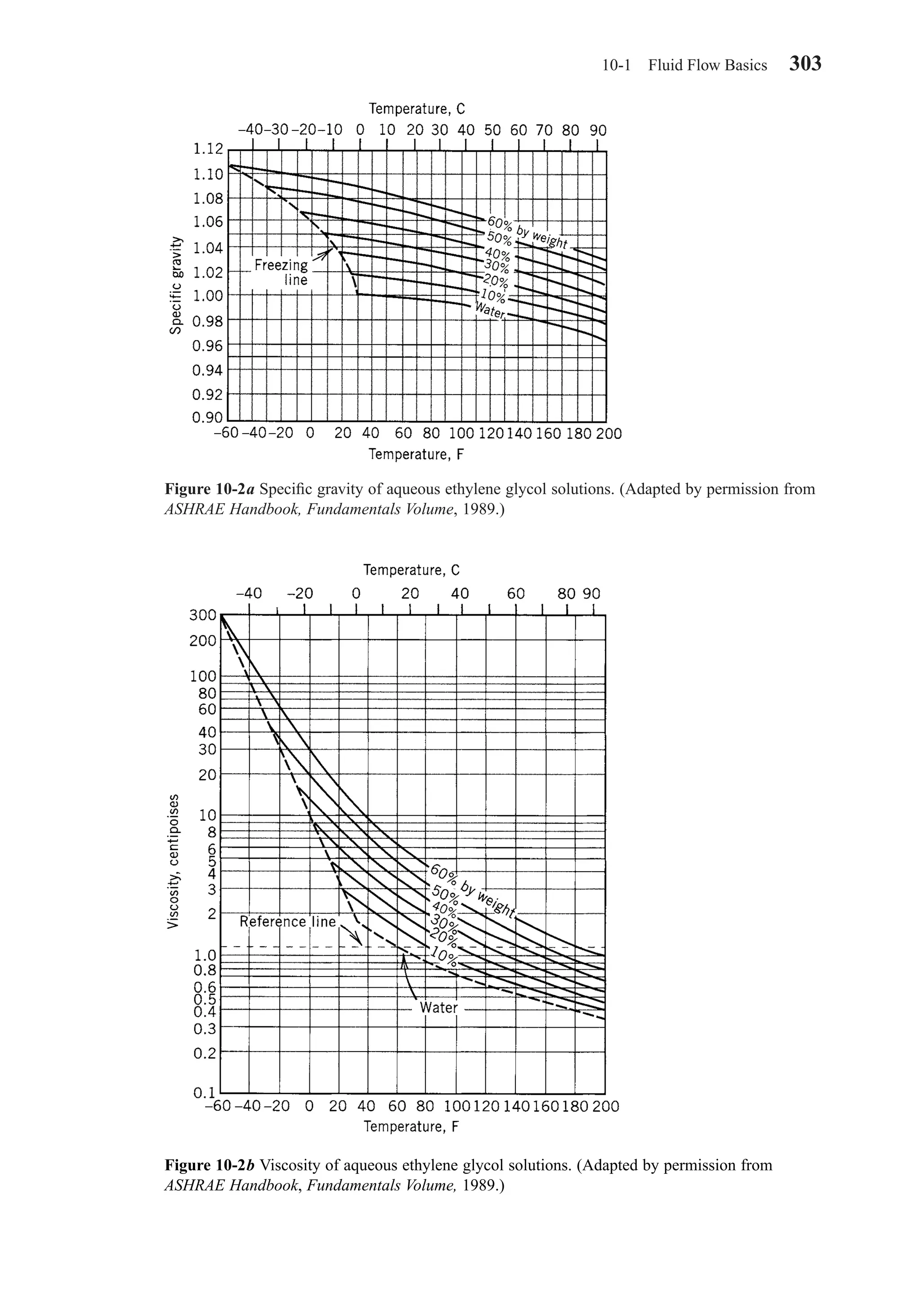
![viscosity data for water and various solutions of ethylene glycol and water. Note that
the viscosity is given in centipoise [1 lbm/(ft-sec) = 1490 centipoise and 103 centipoise
= 1 (N-s)/m2]. The following example demonstrates calculation of lost head for pipe
flow.
EXAMPLE 10-1
Compare the lost head for water and a 30 percent ethylene glycol solution flowing at
the rate of 110 gallons per minute (gpm) in a 3 in. standard (Schedule 40) commer-
cial steel pipe 200 ft in length. The temperature of the water is 50 F.
SOLUTION
Equation 10-6 will be used. From Table C-1 the inside diameter of 3 in. nominal diam-
eter Schedule 40 pipe is 3.068 in. and the inside cross-sectional area for flow is 0.0513
ft2. The Reynolds number is given by Eq. 10-10, and the average velocity in the pipe is
The absolute viscosity of pure water at 50 F is 1.4 centipoise, or 9.4 × 10⁻⁴ lbm/
(ft-sec), from Fig. 10-2b. Then
From Fig. 10-1 the absolute roughness e is 0.00015 for commercial steel pipe. The
relative roughness is then
e/D = 12(0.00015/3.068) = 0.00058
The flow is in the transition zone, and the friction factor f is 0.021 from Fig. 10-1. The
lost head for pure water is then computed using Eq. 10-6:
The absolute viscosity of the 30 percent ethylene glycol solution is 3.1 centipoise from
Fig. 10-2b, and its specific gravity is 1.042 from Fig. 10-2a. The Reynolds number for
this case is
and the friction factor is 0.024 from Fig. 10-1. Then
The increase in lost head with the brine solution is
Percent increase
100(6.94 5.83)
5.83
19 percent=
−
=
lfe = × × =
=
0 024
200
3 068 12
4 78
2 32 2
6 66
6 94
2
.
. /
( . )
( . )
.
.
ft of E.G.S.
ft of water
Re
. ( . ) ( . ) ( . / )
. /
.= = ×
1 042 62 4 4 78 3 068 12
3 1 1490
3 8 104
lfw = × × =0 021
200
3 068 12
4 78
2 32 2
5 83
2
.
. /
( . )
( . )
. ft of water
Re
. ( . ) ( . / )
.
.=
×
= ×−
62 4 4 78 3 068 12
9 4 10
8 1 104
4
V
Q
A
= = = =
˙
( .
.
110
7 48 5
287 4 78
gal/min
gal/ft )(0.0 13ft )
ft/min ft/sec3 2
304 Chapter 10 Flow, Pumps, and Piping Design
Chapter10.qxd 6/15/04 2:32 PM Page 304](https://image.slidesharecdn.com/fayec-160521192803/75/Faye-c-mc_quiston_-_jerald_d-_parker_-_jeffrey_d-322-2048.jpg)
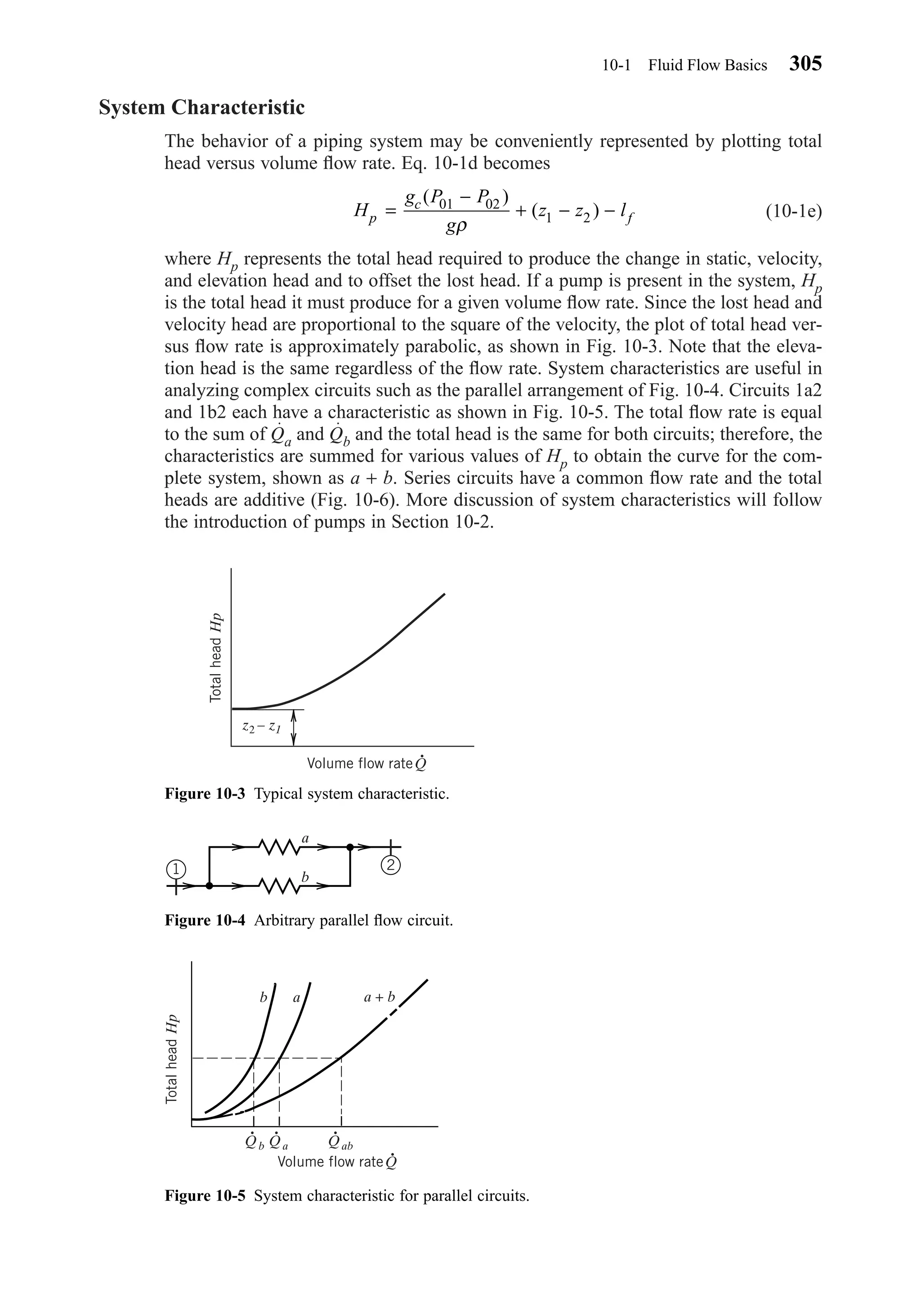
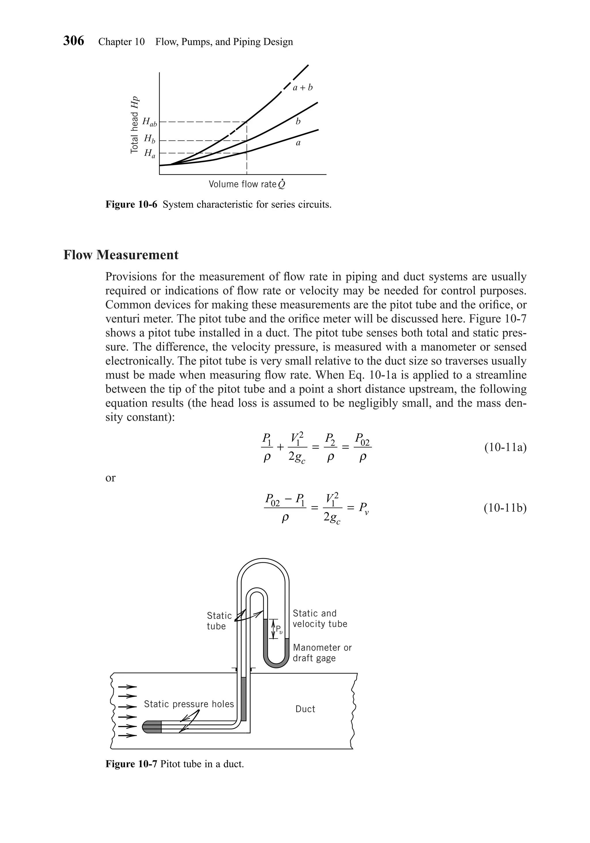
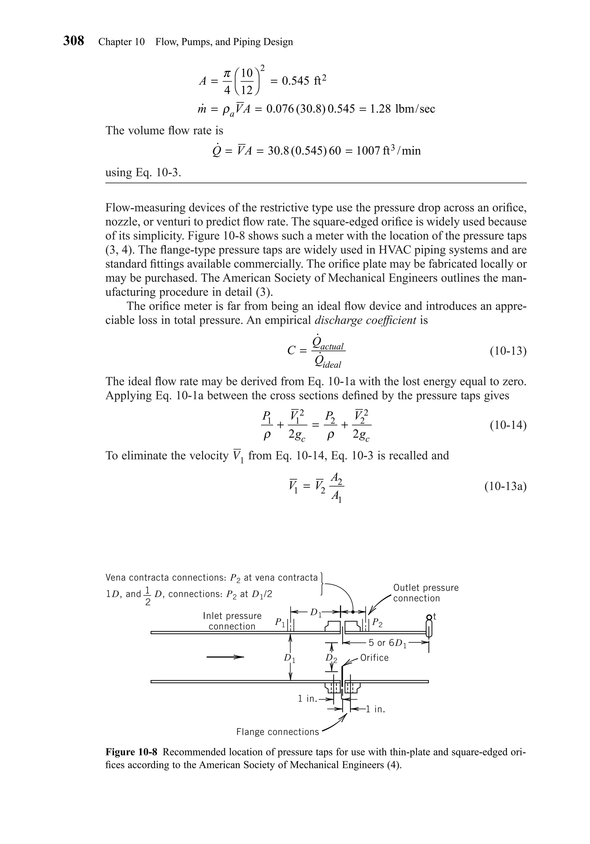
![Substitution of Eq. 10-3 into Eq. 10-14 and rearrangement yields
(10-15)
Then by using Eqs. 10-13 and 10-15 we get
(10-16)
The quantity [1 – (A2/A1)2]1/2 is referred to as the velocity-of-approach factor. In prac-
tice the discharge coefficient and velocity-of-approach factor are often combined and
called the flow coefficient Cd:
(10-17)
This is merely a convenience. For precise measurements other corrections and factors
may be applied, especially for compressible fluids (3, 4). Figure 10-9 shows repre-
sentative values of the flow coefficient Cd. The data apply to pipe diameters over a
wide range (1 to 8 in.) and to flange or radius taps within about 5 percent. When pre-
cise flow measurement is required, the American Society of Mechanical Engineers
Standards (3, 4) should be consulted for more accurate flow coefficients.
Venturi meters are also widely used for flow measurement and control purposes.
They operate on the same principle as orifice meters but with higher flow coefficients
due to a more streamlined design. The American Society of Mechanical Engineers
covers these devices (3, 4). There are specialty balancing valves with pressure taps and
calibration data that are frequently used in piping systems. They operate on the same
principle as orifice meters.
C
C
A Ad =
−[ ( / ) ] /1 2 1
2 1 2
˙
[ ( / ) ] /
/
Q
CA
A A
g
P P
cactual =
−
−
2
2 1
2 1 2
1 2
1 2
1
2
ρ
V
A A
g
P P
c2
2 1
2 1 2
1 2
1 2
1
1
2=
−
−
[ ( / ) ] /
/
ρ
10-1 Fluid Flow Basics 309
Figure 10-9 Flow coefficients for square-edged orifices.
40,000 80,000 120,000 160,000 200,000 240,000
D1
= 0.60
D2
D1
= 0.55
D2
D1
= 0.40
D2
D1
= 0.20
D2
0.67
0.66
0.65
0.64
0.63
0.62
0.61
0.60
0.59
0
FlowcoefficientCd
Reynolds number =
ρ
µ
V2D2
–
Chapter10.qxd 6/15/04 2:32 PM Page 309](https://image.slidesharecdn.com/fayec-160521192803/75/Faye-c-mc_quiston_-_jerald_d-_parker_-_jeffrey_d-327-2048.jpg)
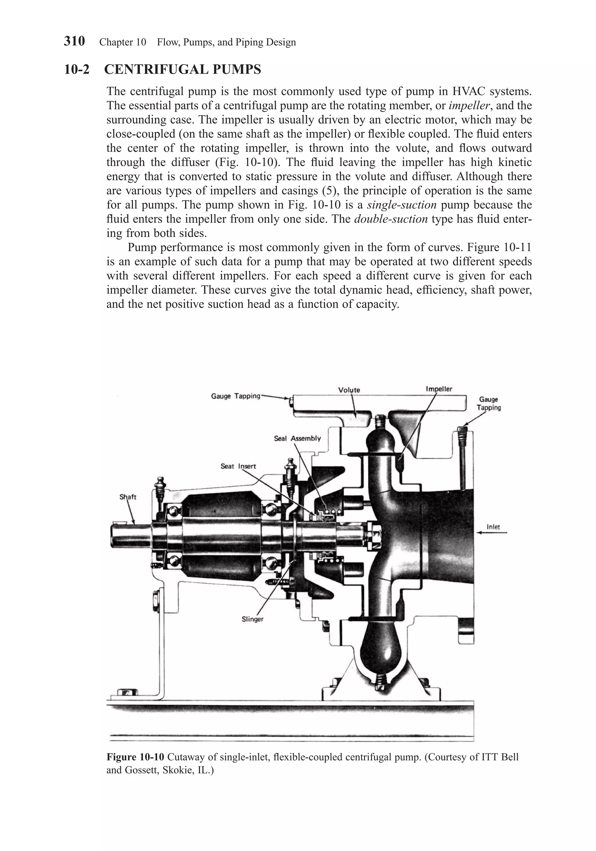
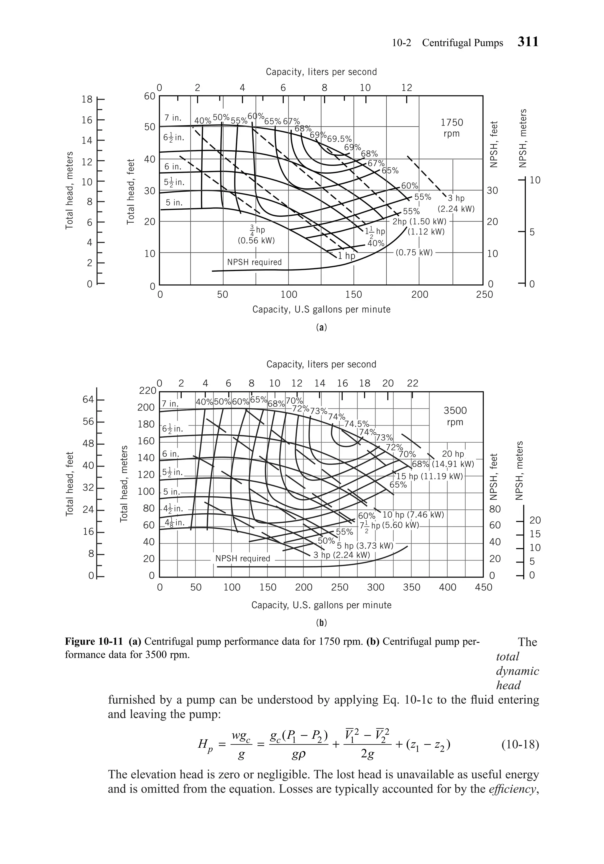
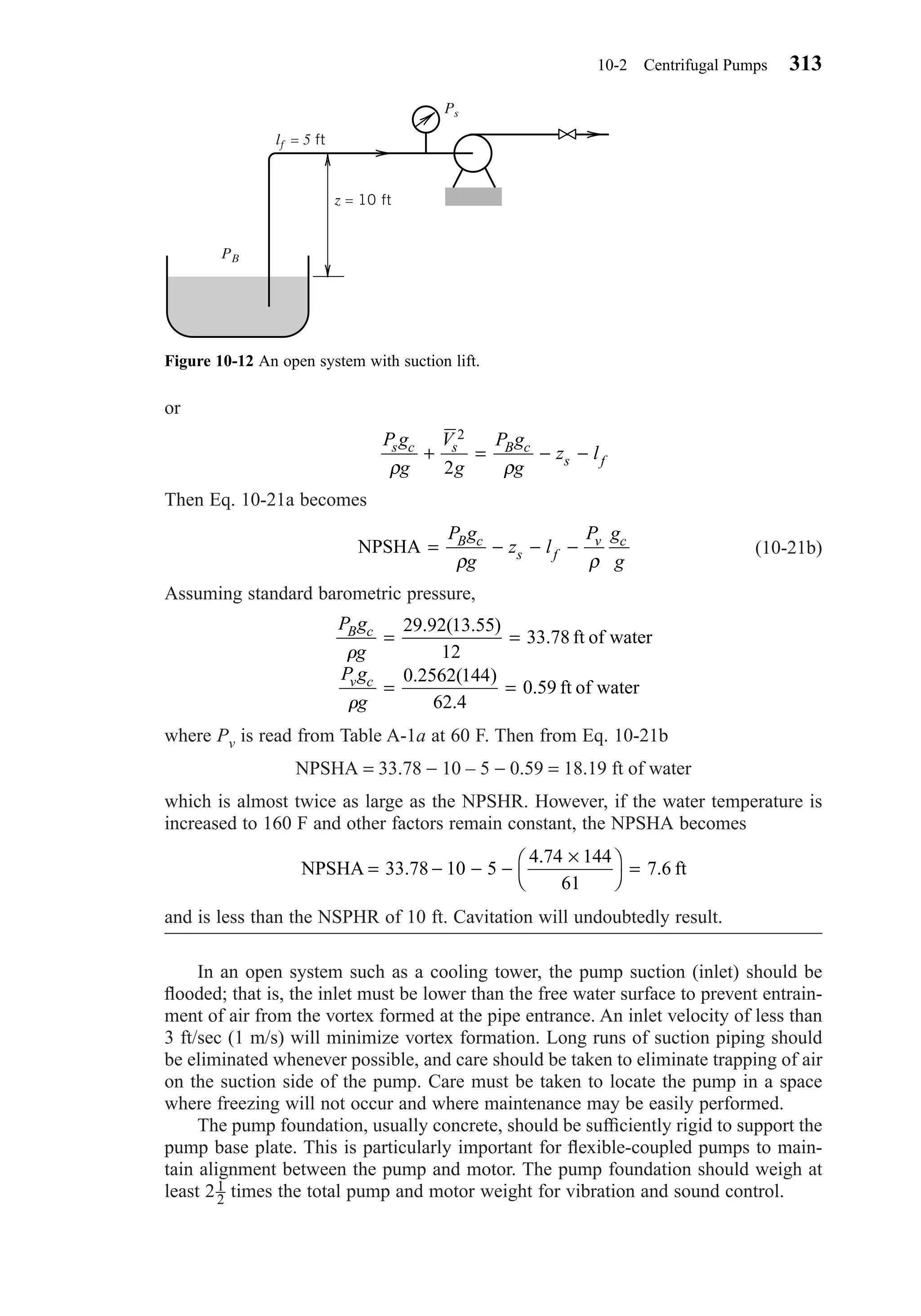
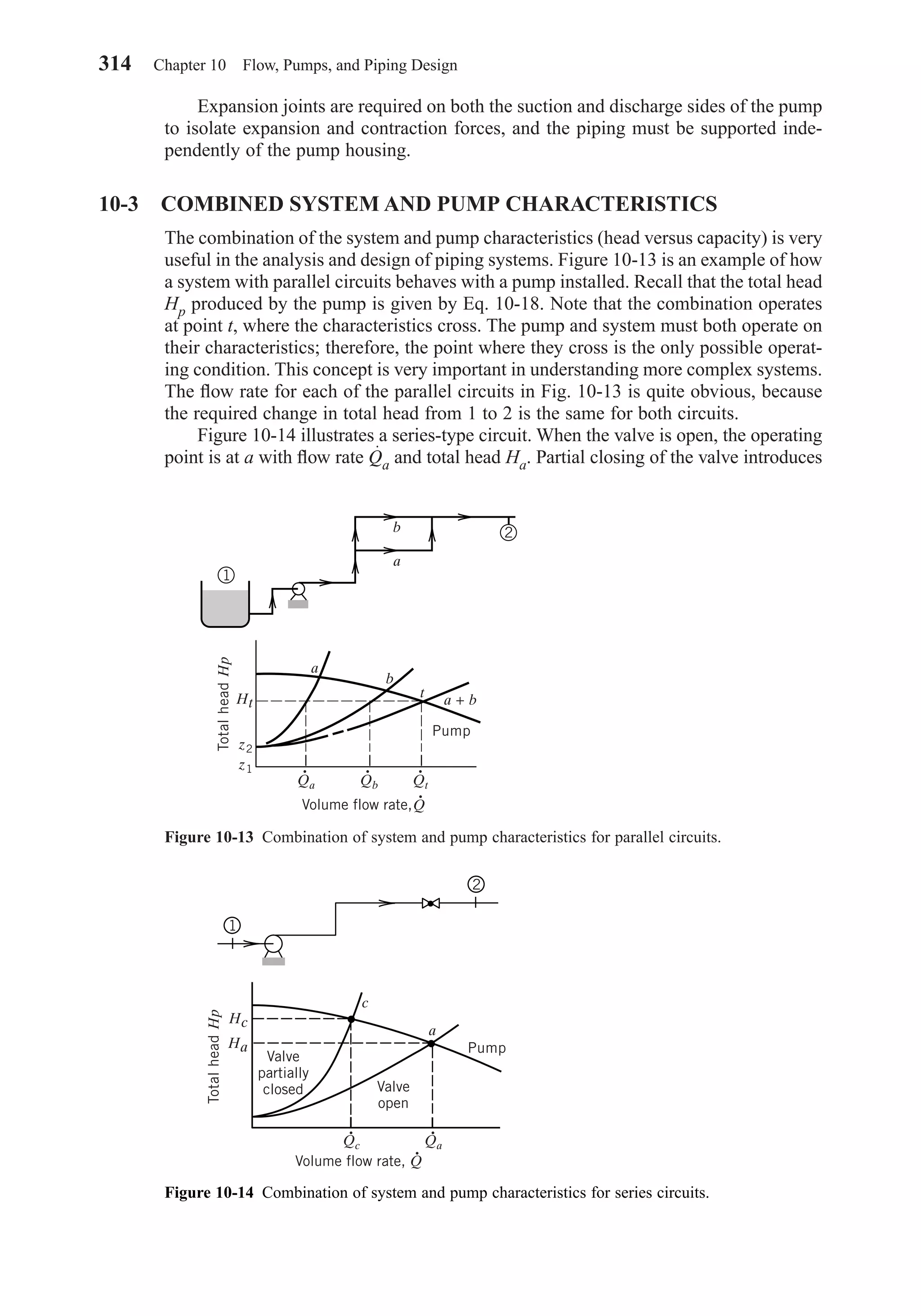
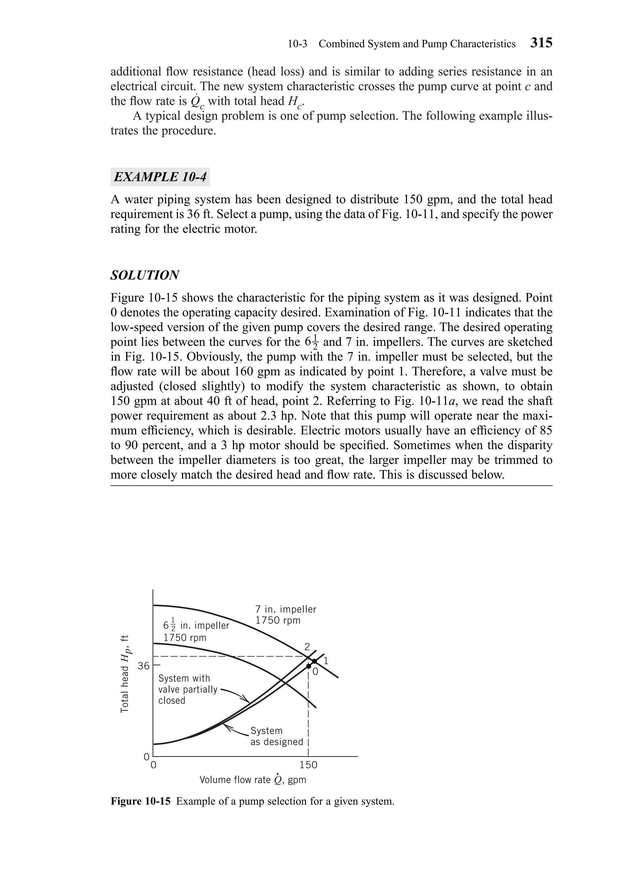
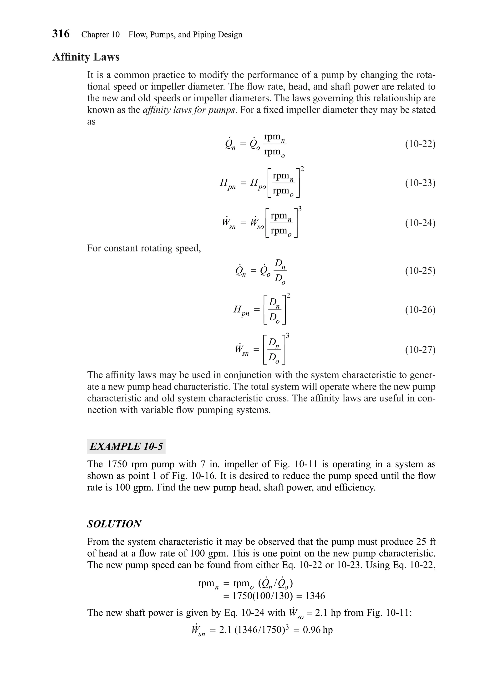
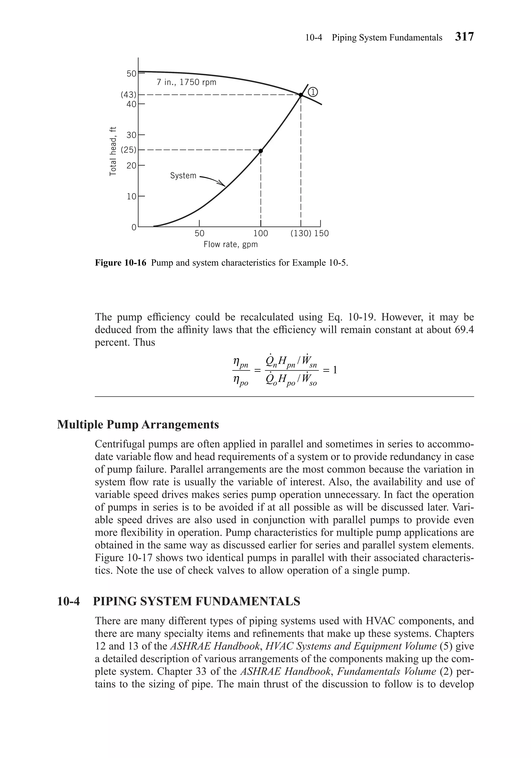
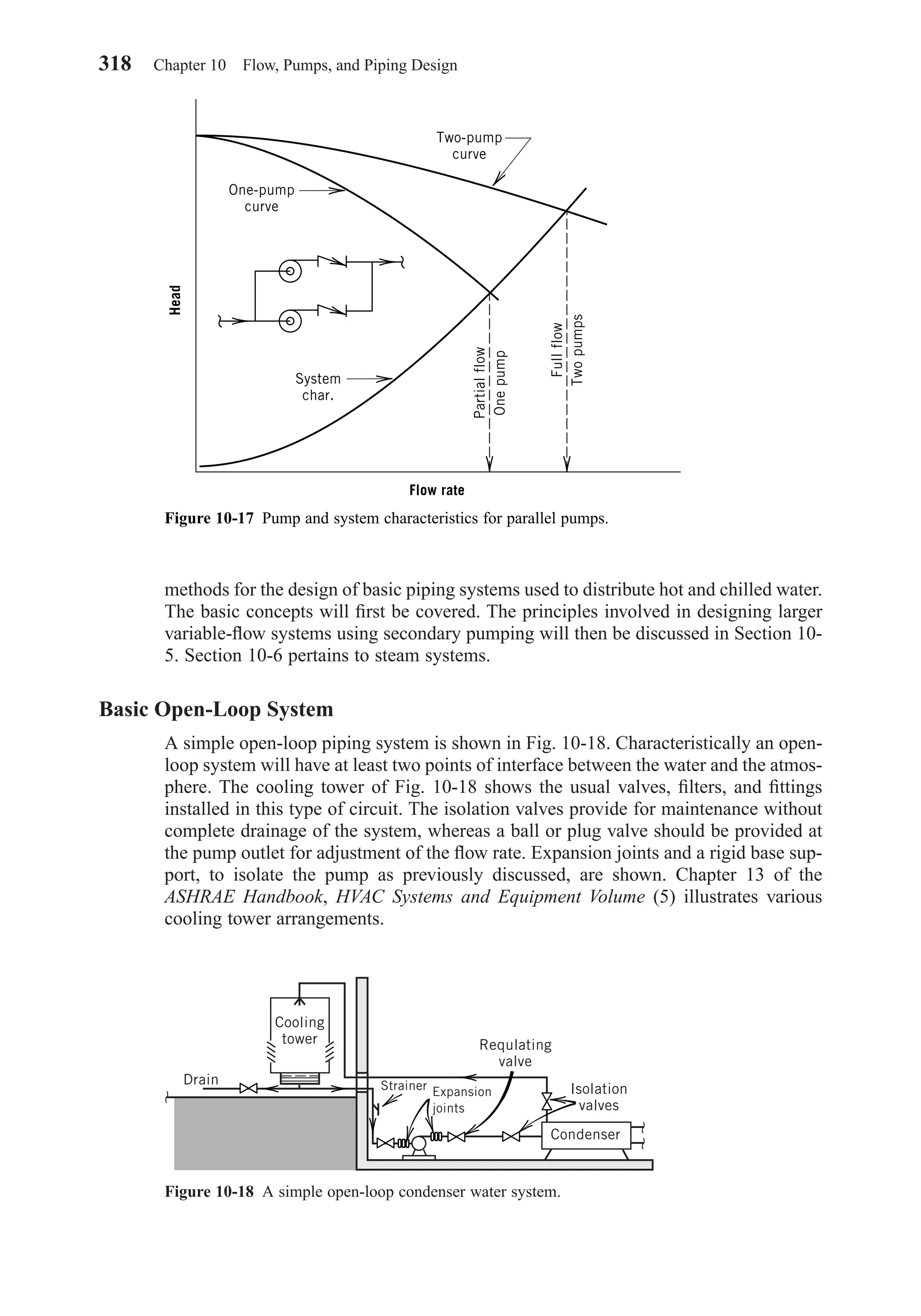
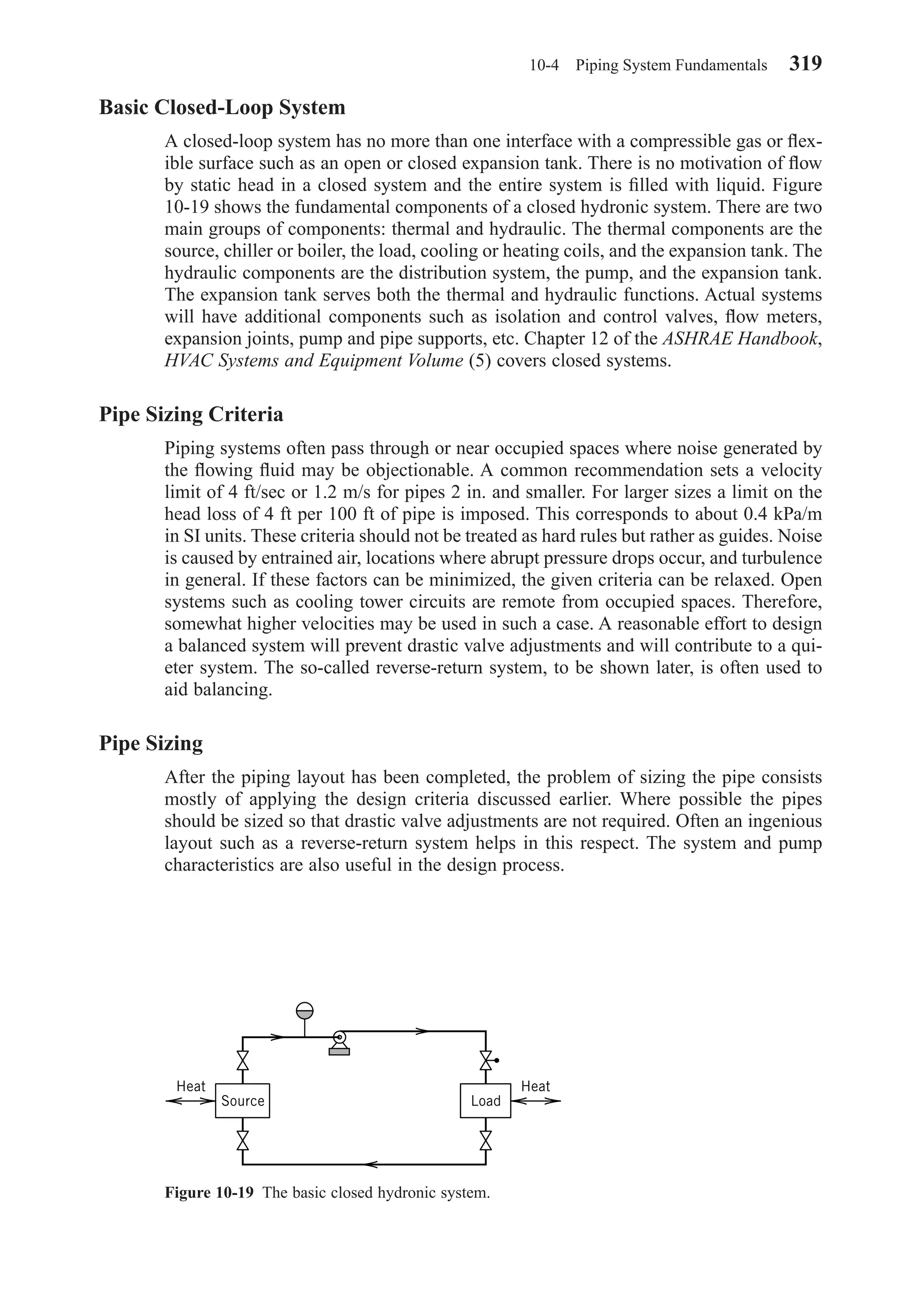
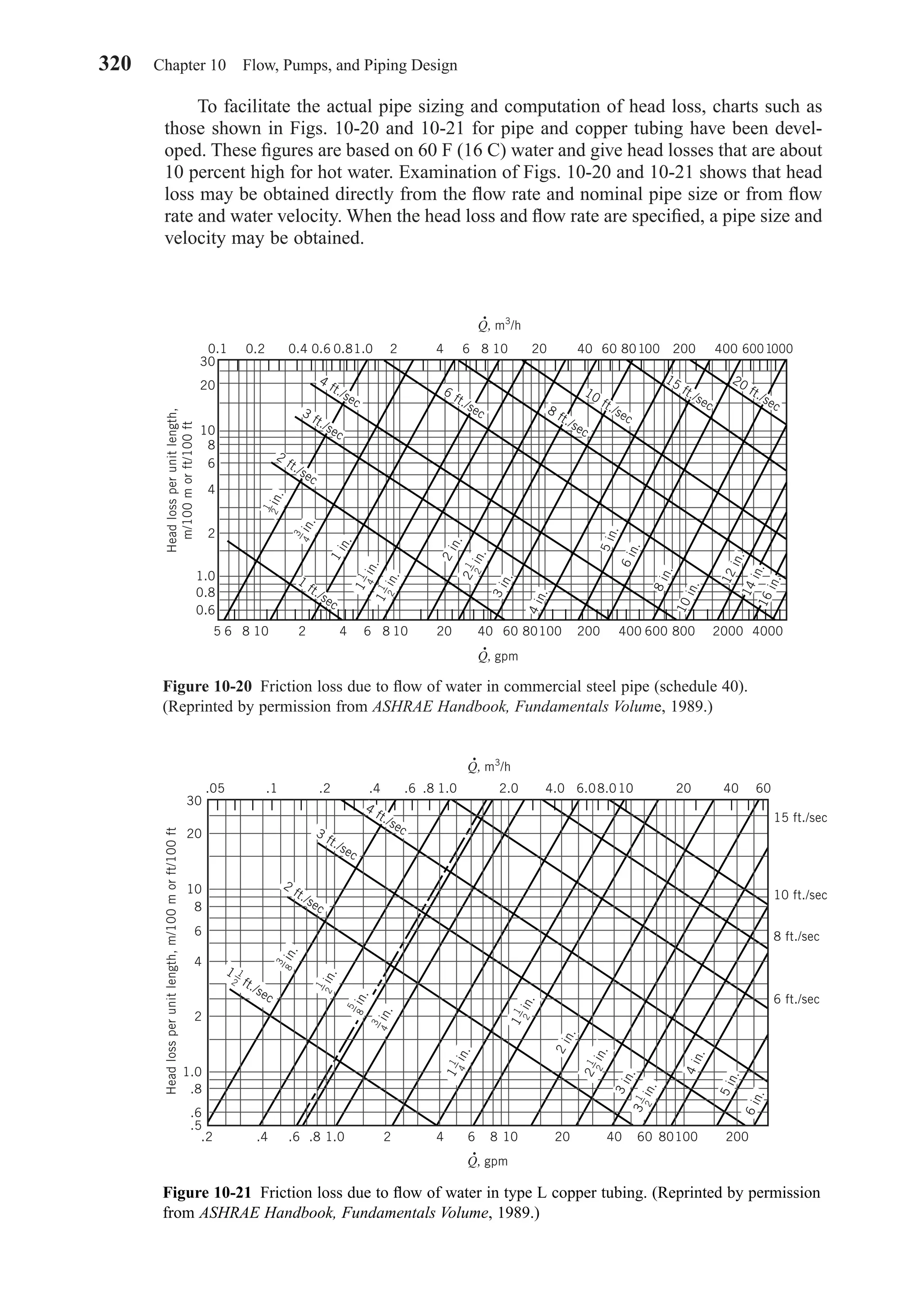

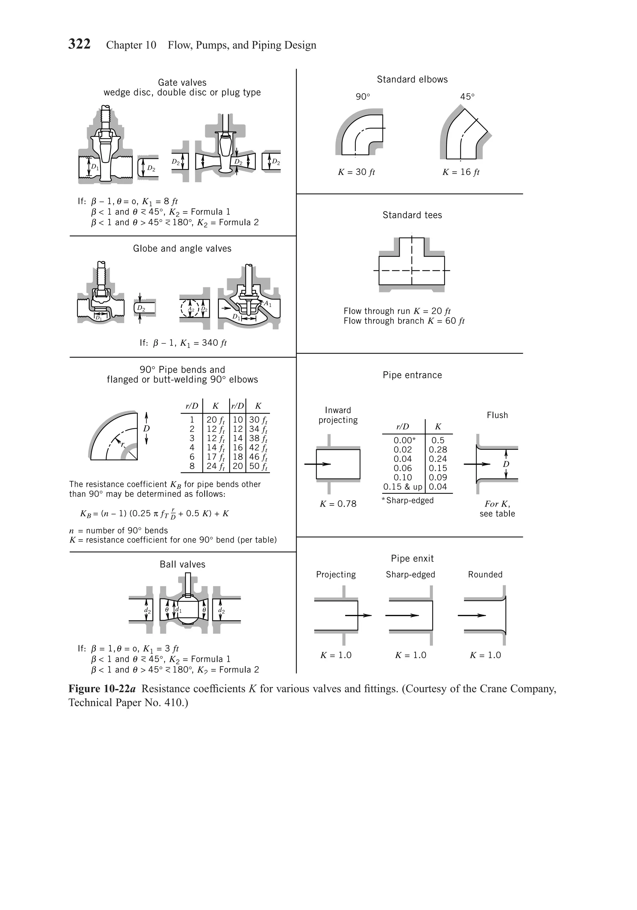
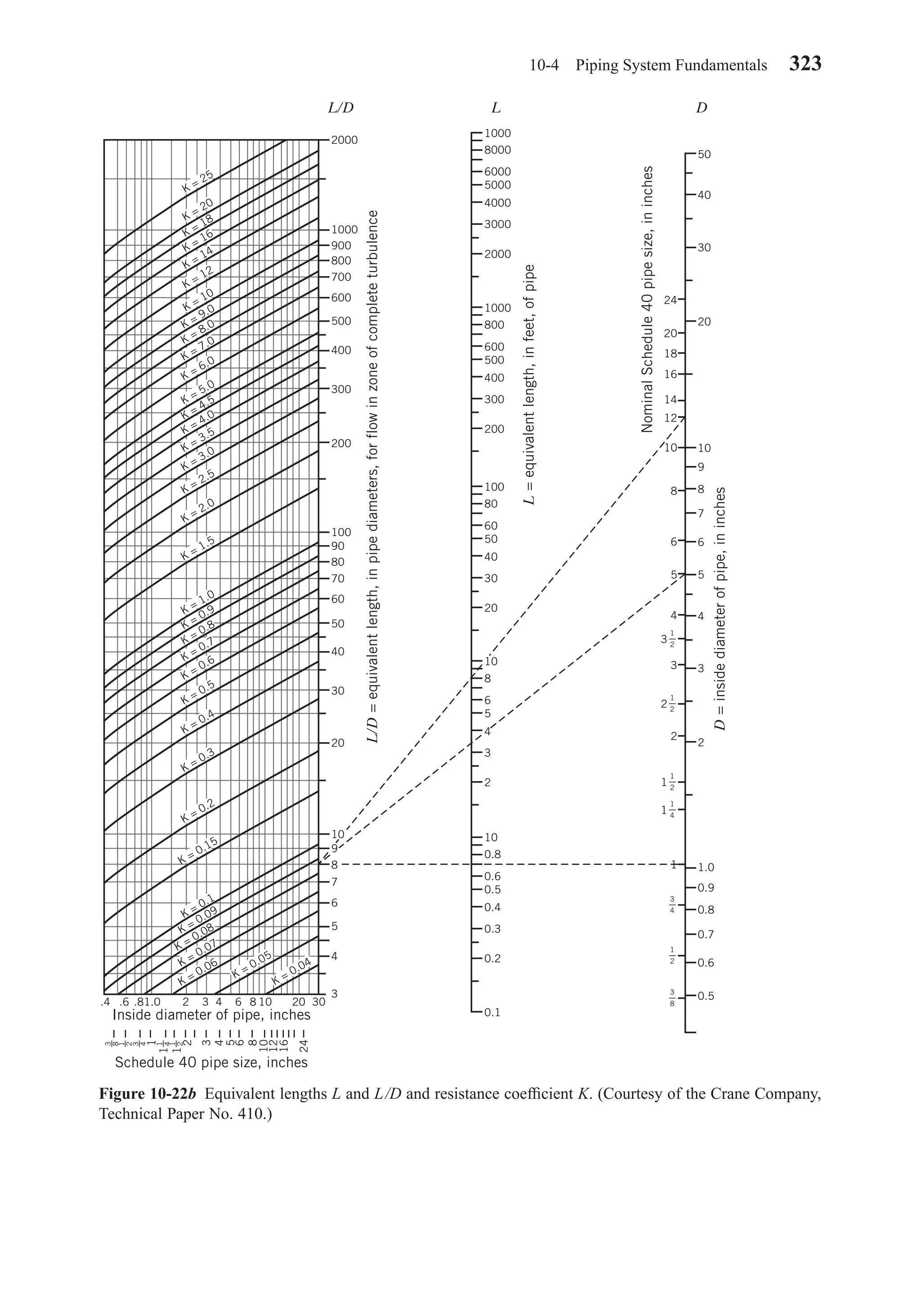
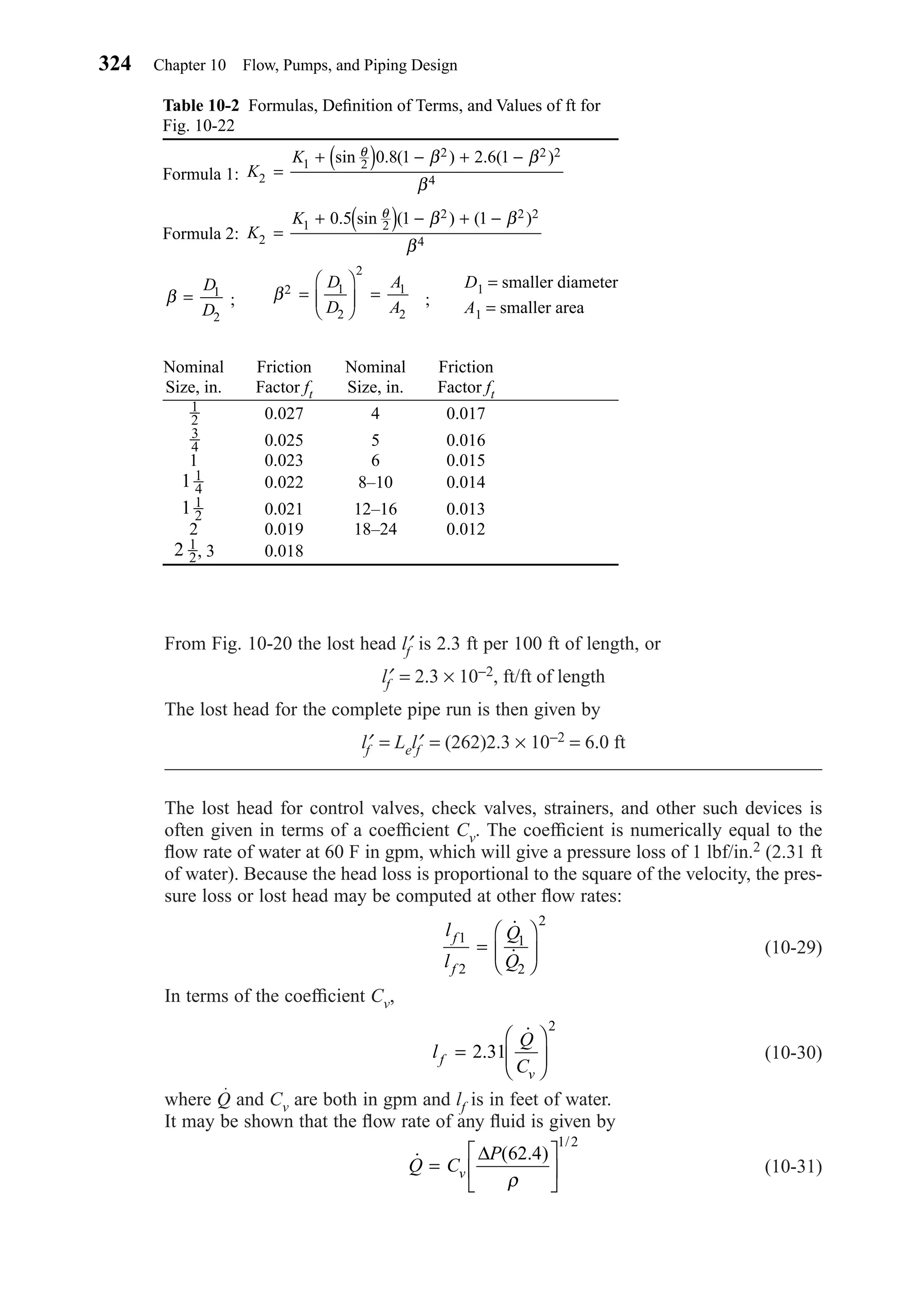
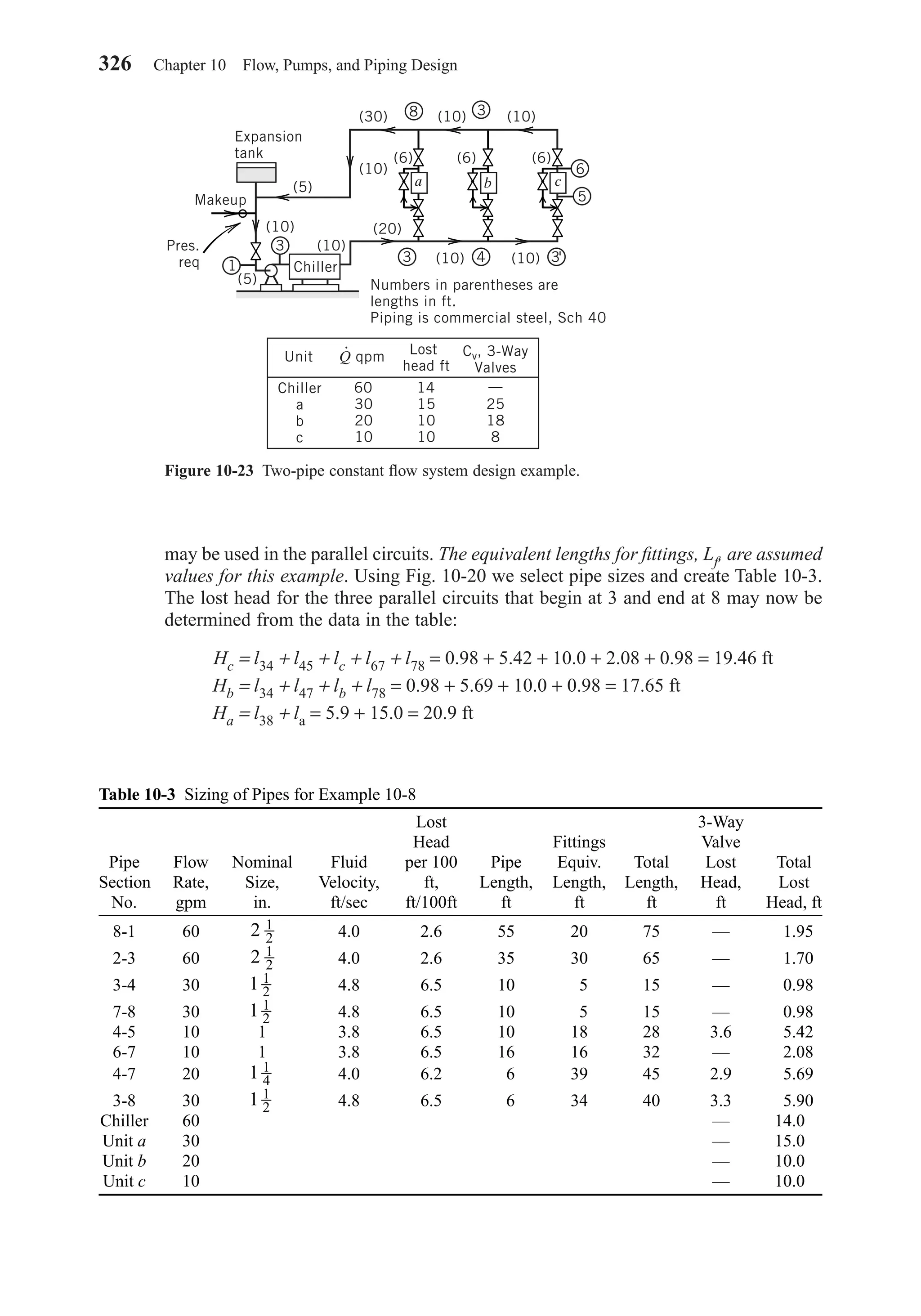
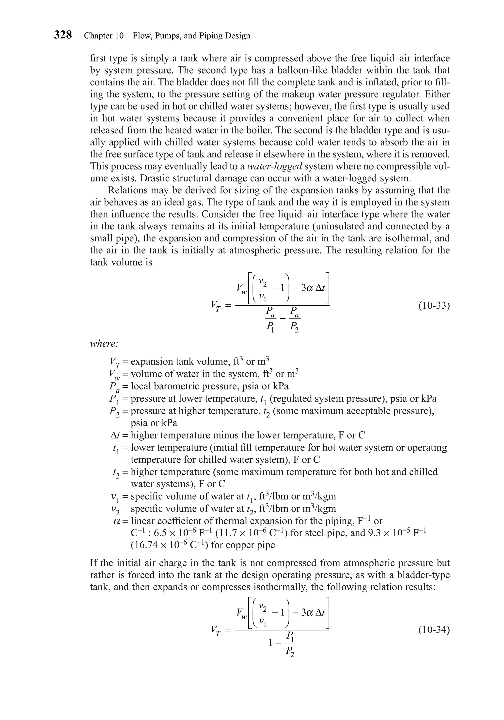
![where the variables are defined as for Eq. 10-33.
The expansion tank must be installed so that the assumptions made in deriving
Eqs. 10-33 and 10-34 are valid. This generally means that the expansion tank is not
insulated and is connected to the main system by a relatively long, small-diameter pipe
so that water from the system does not circulate into the expansion tank. The follow-
ing example demonstrates the expansion tank problem.
EXAMPLE 10-9
Compute the expansion tank volume for a chilled water system that contains 2000 gal
of water. The system is regulated to 10 psig at the tank with an operating temperature
of 45 F. It is estimated that the maximum water temperature during extended shut-
down would be 100 F and a safety relief valve in the system is set for 35 psig. Assume
standard barometric pressure and steel pipe.
SOLUTION
A bladder type would be the best choice; however, calculations will be made for both
types. Equation 10-33 will give the volume of the free liquid–air interface type tank
where ν2 = 0.01613 ft3/lbm and ν1 = 0.01602 ft3/lbm from Table A-1a:
Equation 10-34 will give the volume of the bladder-type tank:
Note that the volume of the bladder-type tank is less than the free-surface type. This
is an advantage in large systems.
Air Elimination
Air is a source of problems in closed-circuit liquid circulation systems; therefore,
measures must be taken to eliminate it. The primary source of air is from dissolved
gases in the makeup water to the system. The amount of air that can be dissolved in
water depends on the pressure and temperature of the water as governed by Henry’s
law.
Henry’s law states that the amount of dissolved air at a given pressure varies
inversely with the temperature and depends directly on the pressure at a given tem-
perature. Figure 10-24 illustrates Henry’s law for water. The solubility of dissolved air
is high where the temperature is low and the pressure is high. For example, when cold
tap water at 55 psig (380 kPa) and 40 F (4 C) is added to a system and heated to 120 F
(49 C) with a reduction in pressure to 10 psig (69 kPa), the dissolved air may be
reduced from about 12 percent to about 2 percent. For each 10 gal (38 L) of makeup
water there may be about 1 gal (3.8 L) of air introduced into the system.
V
V
TF
TF
=
−( ) − ×[ ]
−
= =
−2000 1 3 6 5 10 55
1
23 0 3 1
0 01613
0 01602
6
14 696
49 696
3
.
.
.
.
( . ) ( )
. .gal ft
V
V
TF
TF
=
−( ) − ×
−( )
= =
−2000 1 3 6 5 10 55
38 7 5 2
0 01613
0 01602
6
14 696
24 696
14 696
49 696
3
.
.
.
.
.
.
( . ) ( )
. .gal ft
10-4 Piping System Fundamentals 329
Chapter10.qxd 6/15/04 2:33 PM Page 329](https://image.slidesharecdn.com/fayec-160521192803/75/Faye-c-mc_quiston_-_jerald_d-_parker_-_jeffrey_d-347-2048.jpg)

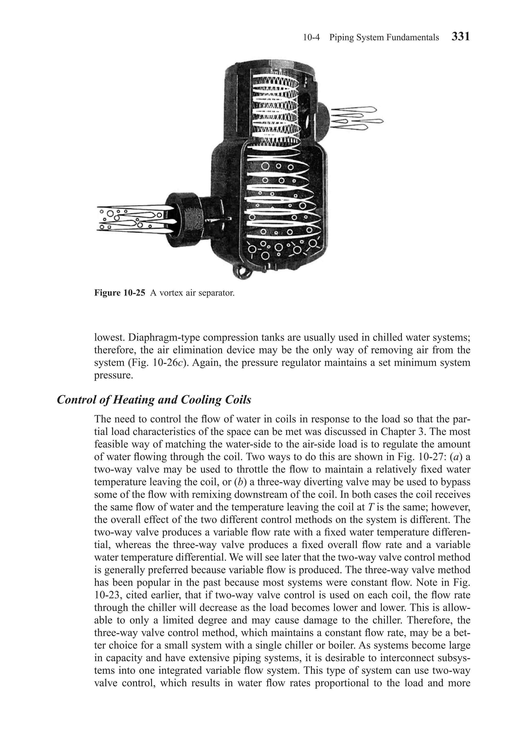
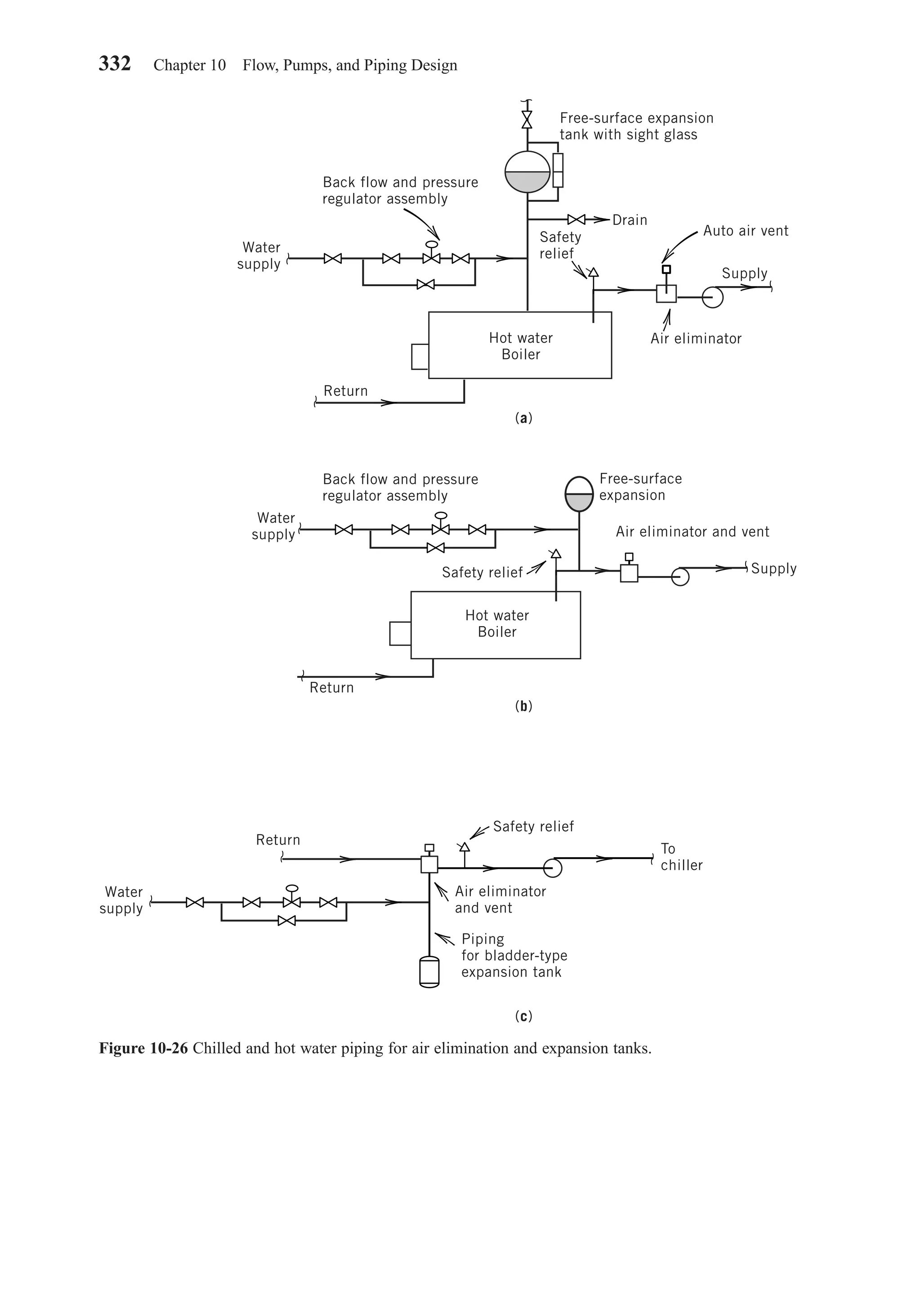
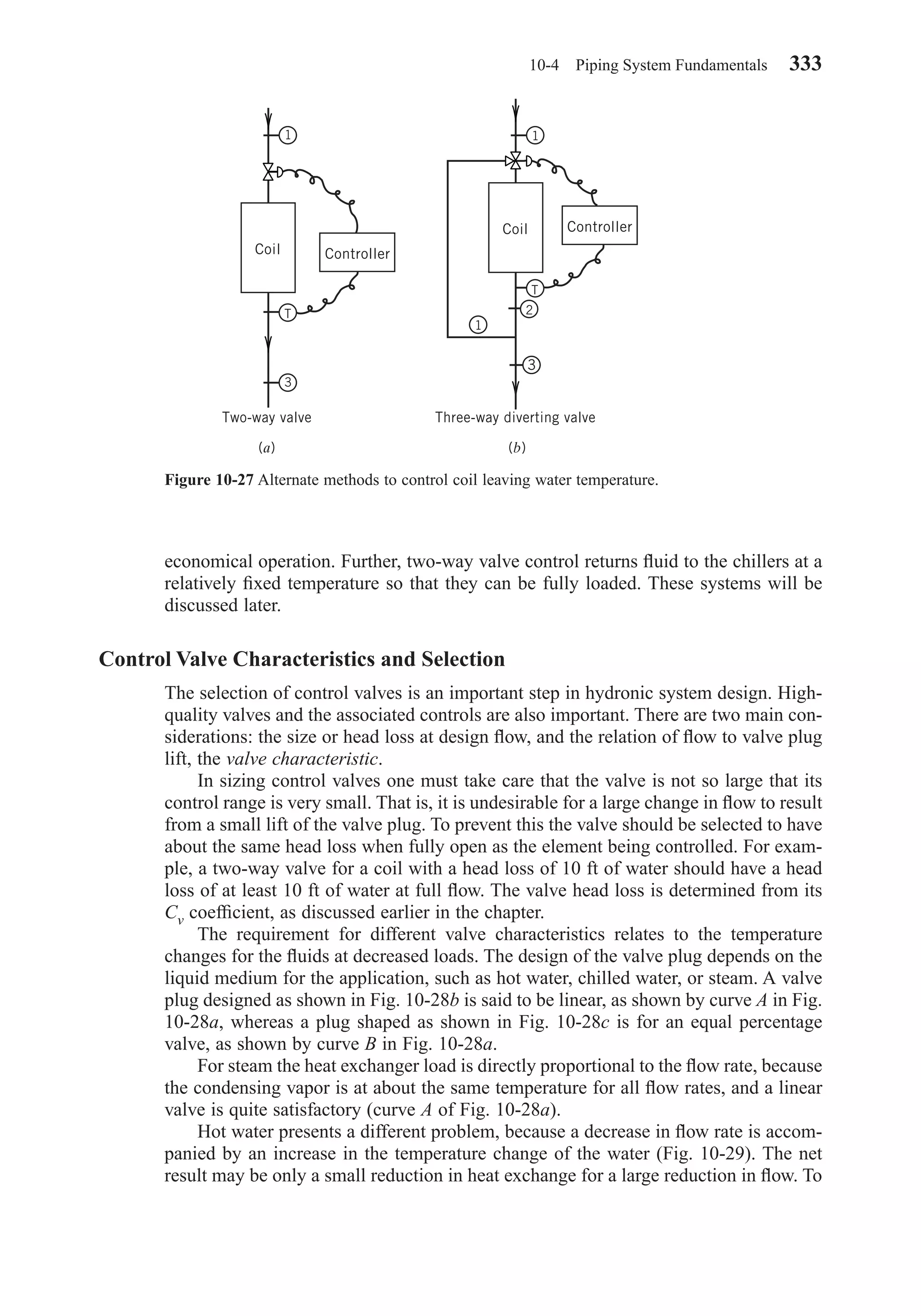
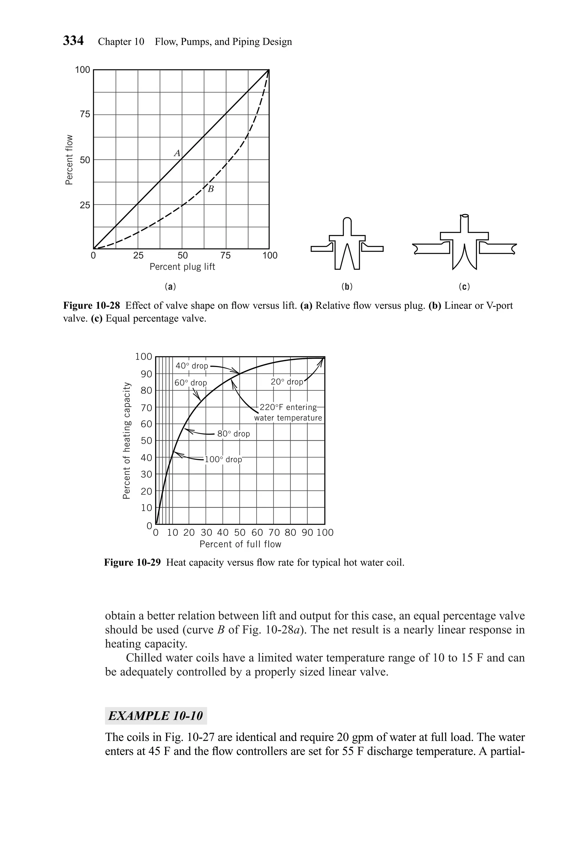
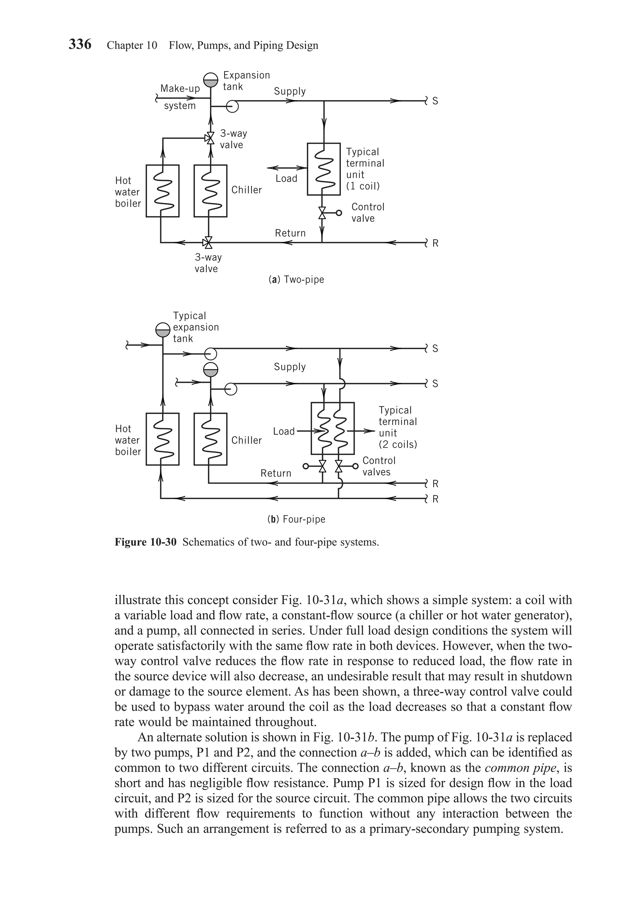
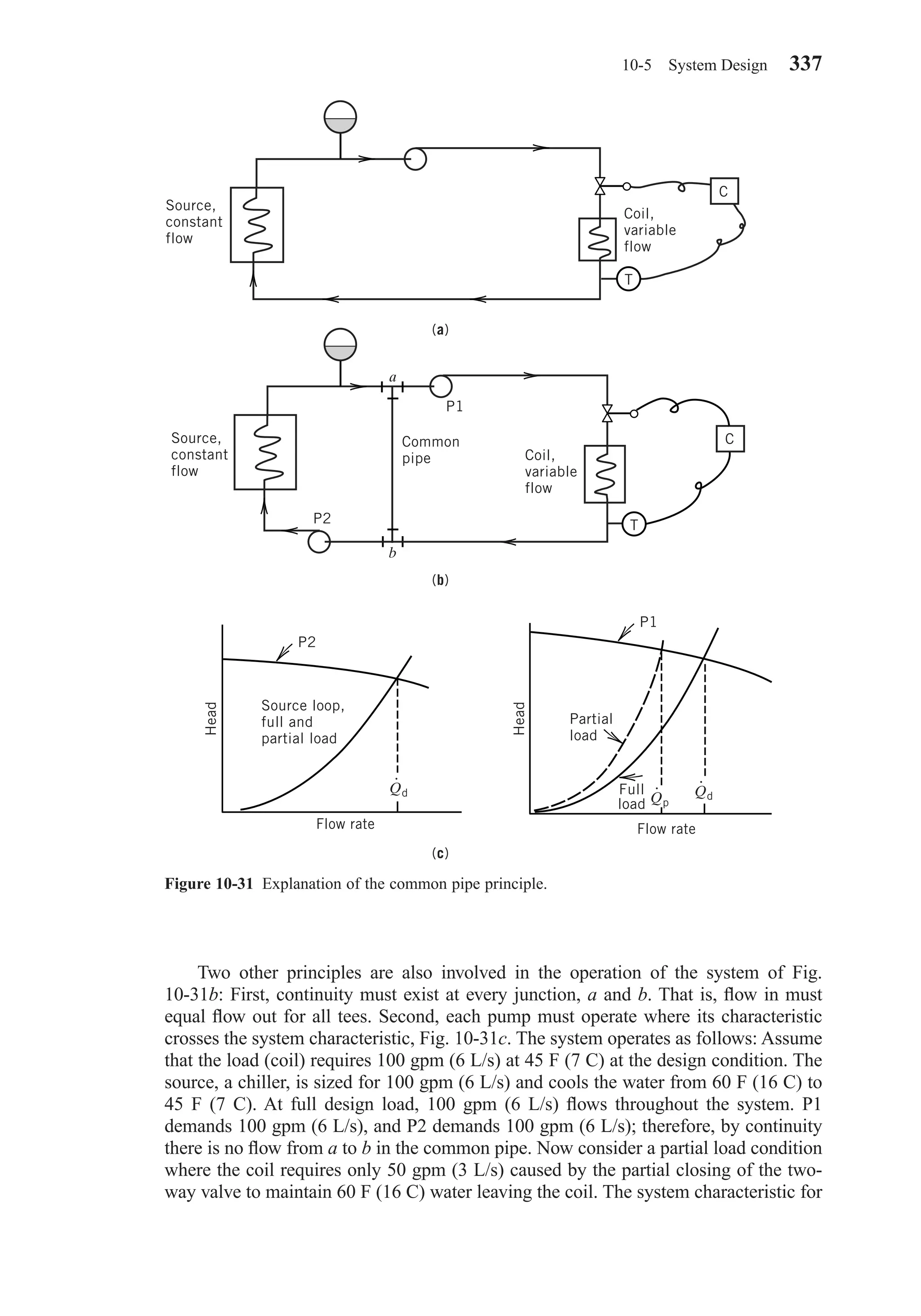
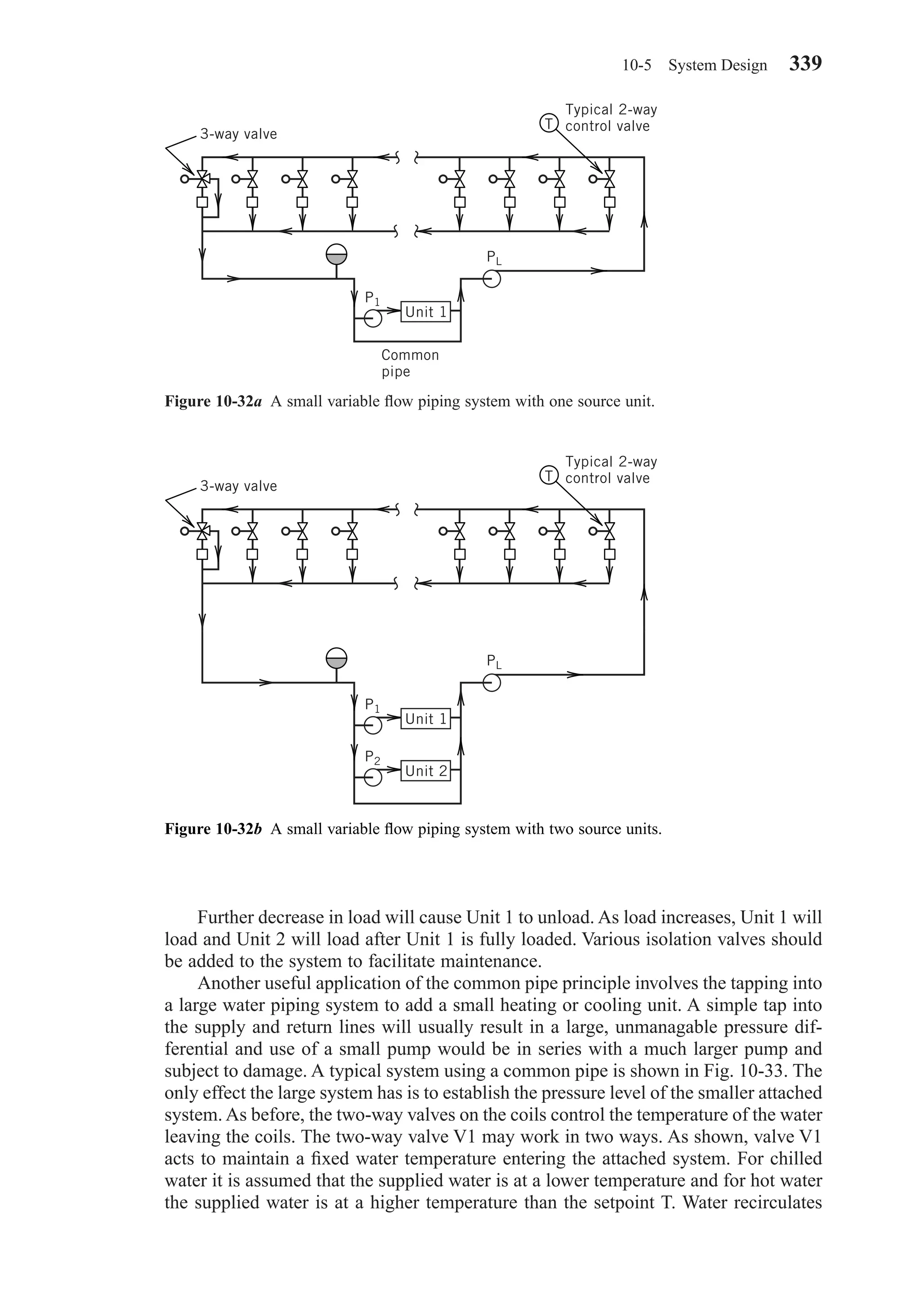
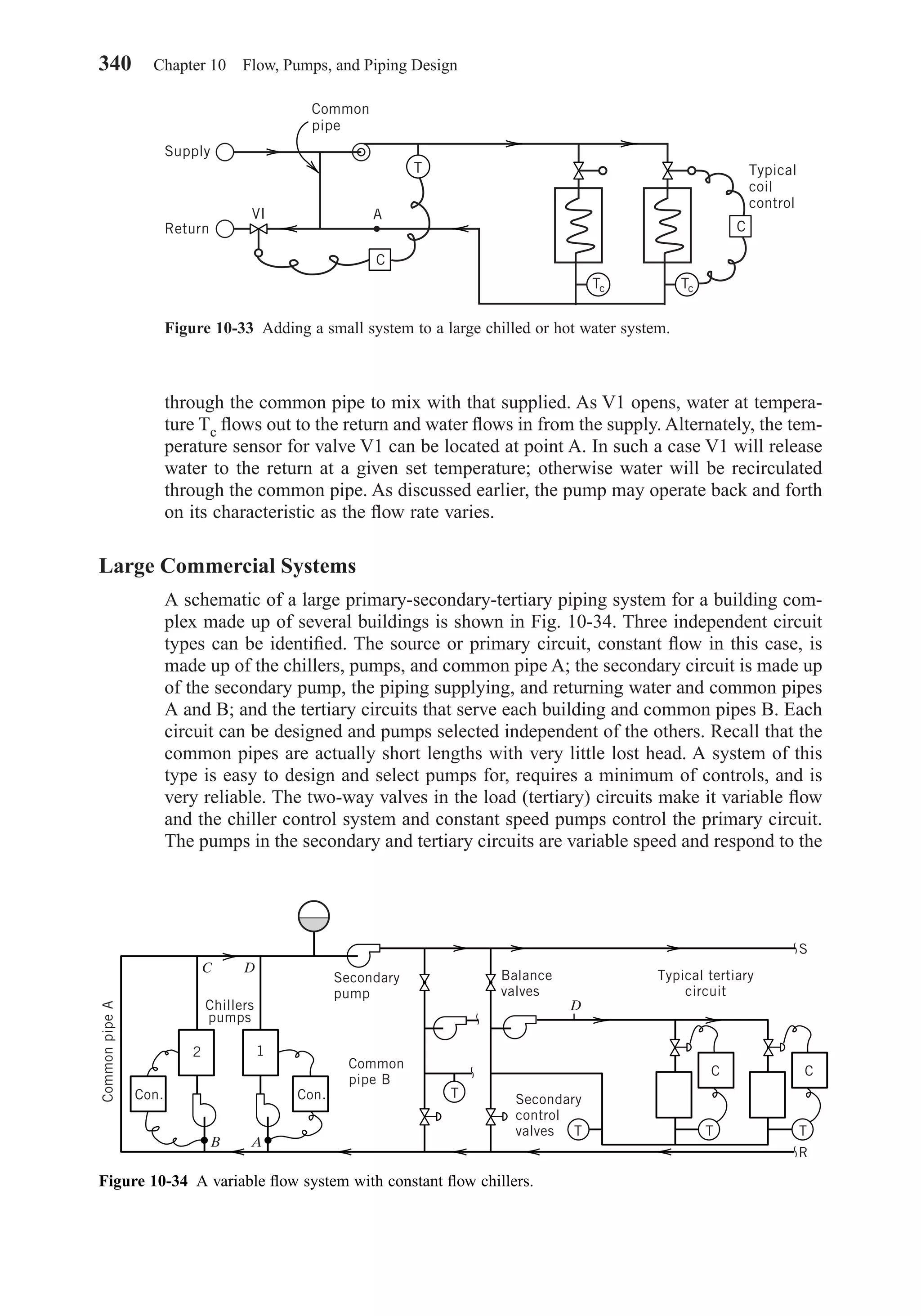
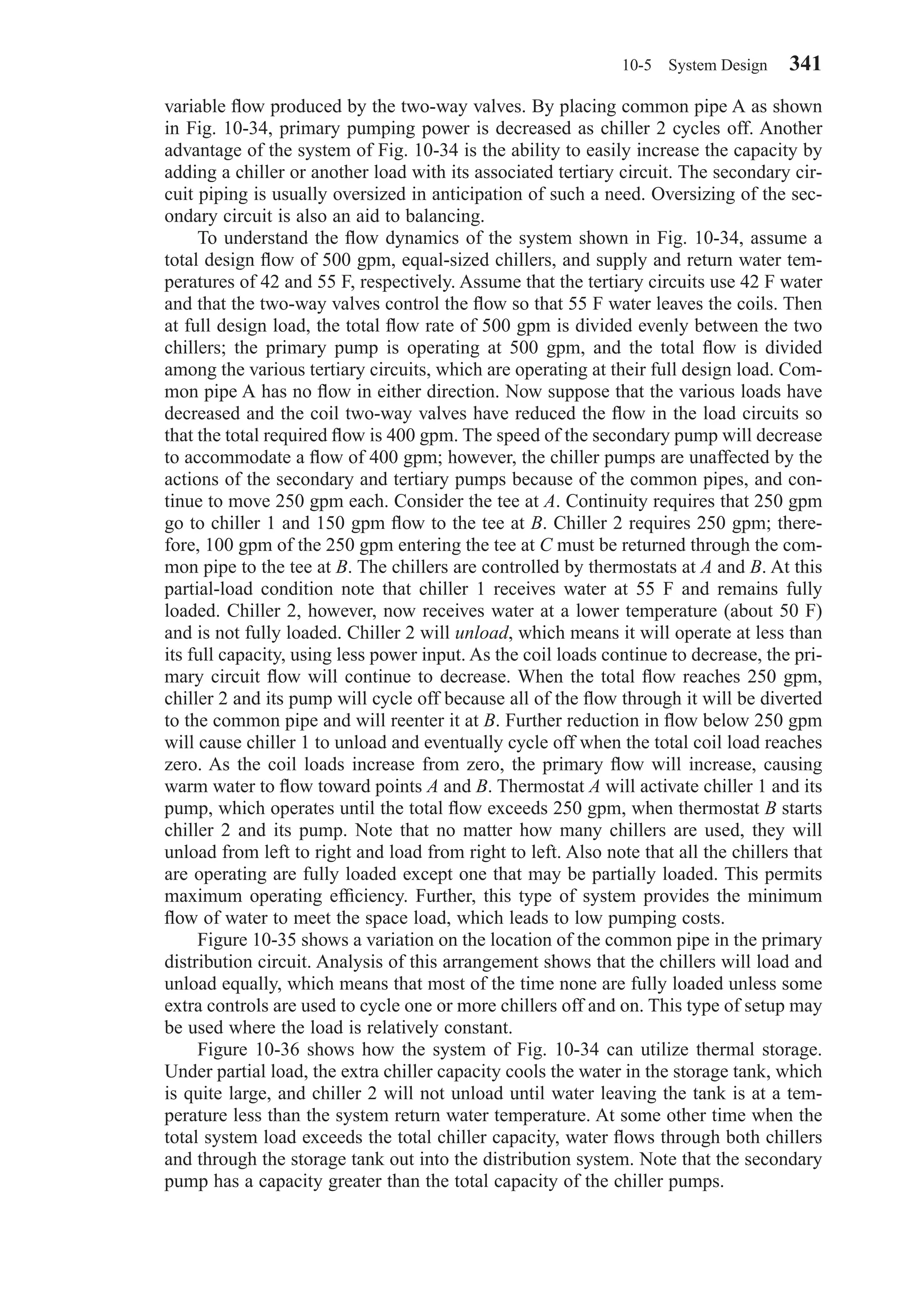

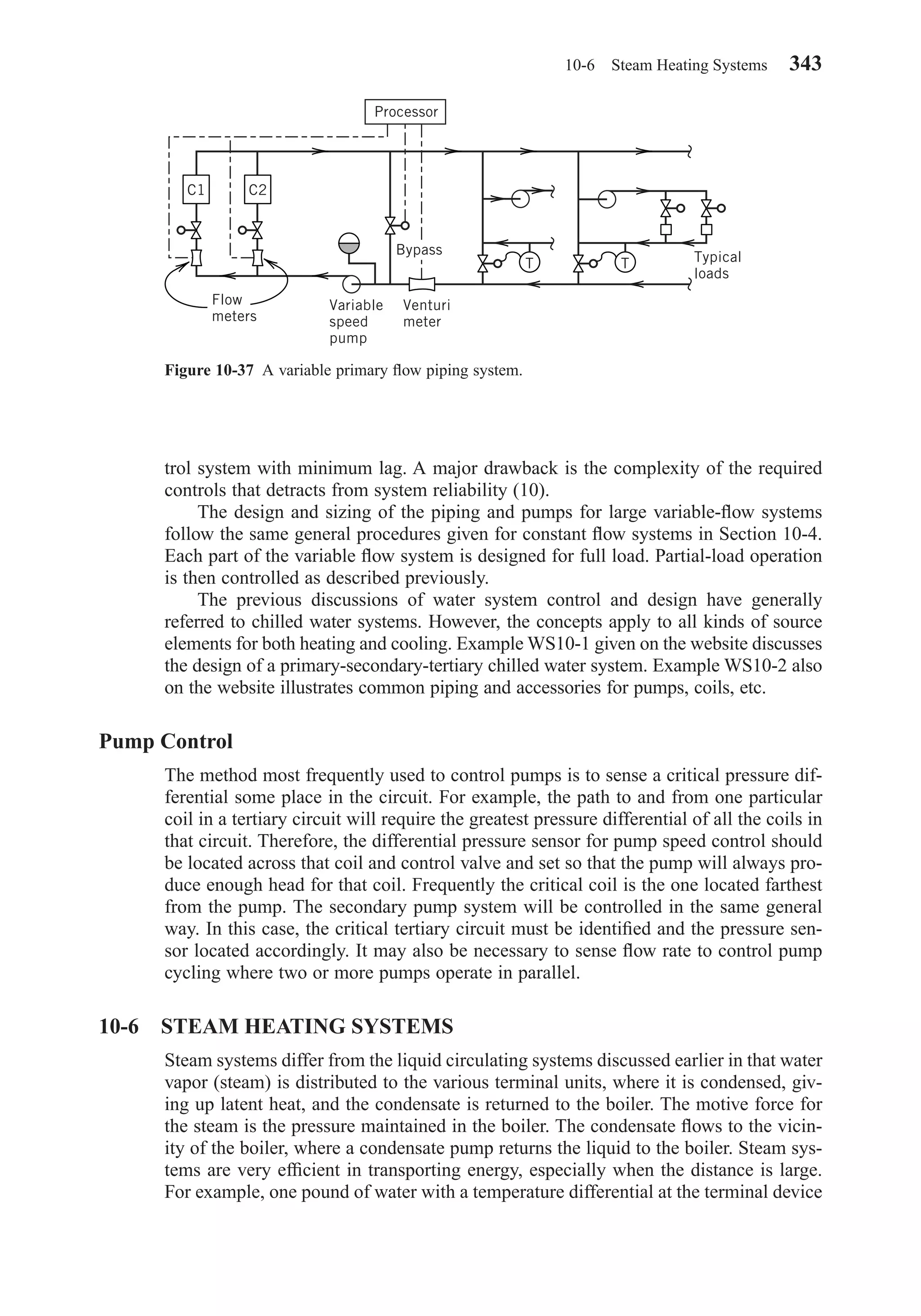
![of 20 F (7 C) releases 20 Btu (6 W-hr) of energy, while one pound of saturated vapor
at 5 psig (35 kPa) releases about 950 Btu (278 W-hr). Other advantages of steam
are: heat transfer at constant temperature, minimum shaft energy required, and a
pressure–temperature dependence that is often helpful for control.
Steam radiators and steam-to-air coils are not as frequently used for space heating
as in the past. Instead, steam may be used to heat water, which is distributed and used
in water-to-air coils. However, there are many steam heating applications in hospitals,
various industrial plants, and the process industry. The emphasis here is on HVAC
applications, where steam is available at low pressure (less than 15 psig [103 kPa]).
The steam piping circuit is somewhat more complicated than a liquid piping cir-
cuit, mainly because two phases, liquid and vapor, are present in the system. To oper-
ate properly, the two phases must be separated except in the boiler. Figure 10-38 is a
schematic of a low-pressure steam circuit.
Condensate Return
A properly operating condensate return circuit is critical to the efficient operation of
the steam system. Saturated vapor will condense whenever it comes in contact with a
surface at a temperature less than the steam temperature. Therefore, even before the
steam reaches the terminal devices, small amounts of condensate will form in the pip-
ing. Devices known as steam traps remove this condensate. A steam trap will allow
liquid to pass through to the condensate return but will retain the steam in the system.
Every terminal device requires a steam trap. The different types of steam traps will be
discussed later.
It is very important that condensate not be allowed to collect in the steam piping,
because of the possibility of water hammer. A slug of condensate may form, completely
344 Chapter 10 Flow, Pumps, and Piping Design
Figure 10-38 Schematic of a low-pressure steam circuit.
Air vent
Air vent
Steam
trap
(typical)
Steam
separator
Boiler
Make up
Feedwater
system
Air
vent
Condensate
return
Chapter10.qxd 6/15/04 2:33 PM Page 344](https://image.slidesharecdn.com/fayec-160521192803/75/Faye-c-mc_quiston_-_jerald_d-_parker_-_jeffrey_d-362-2048.jpg)
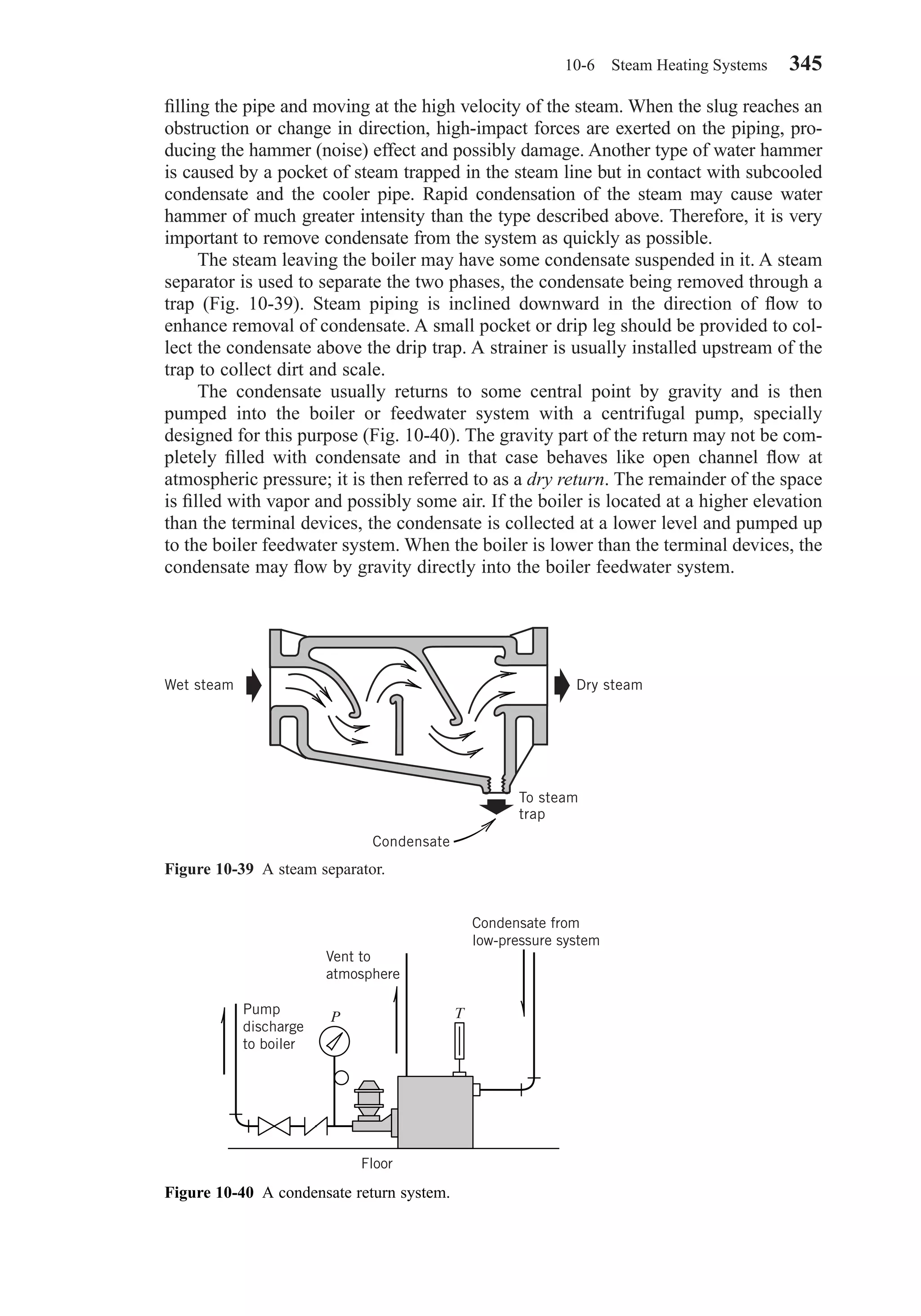
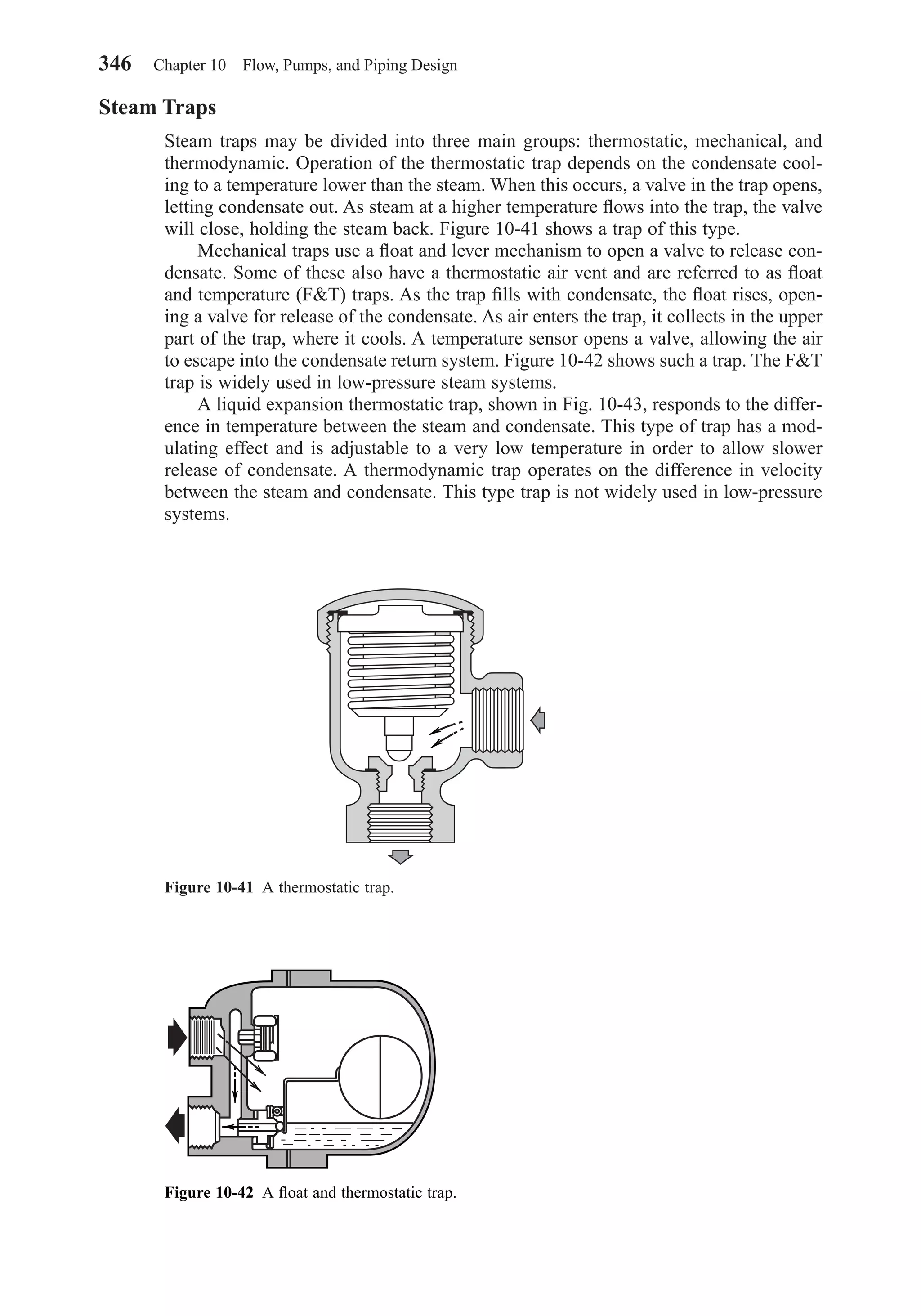
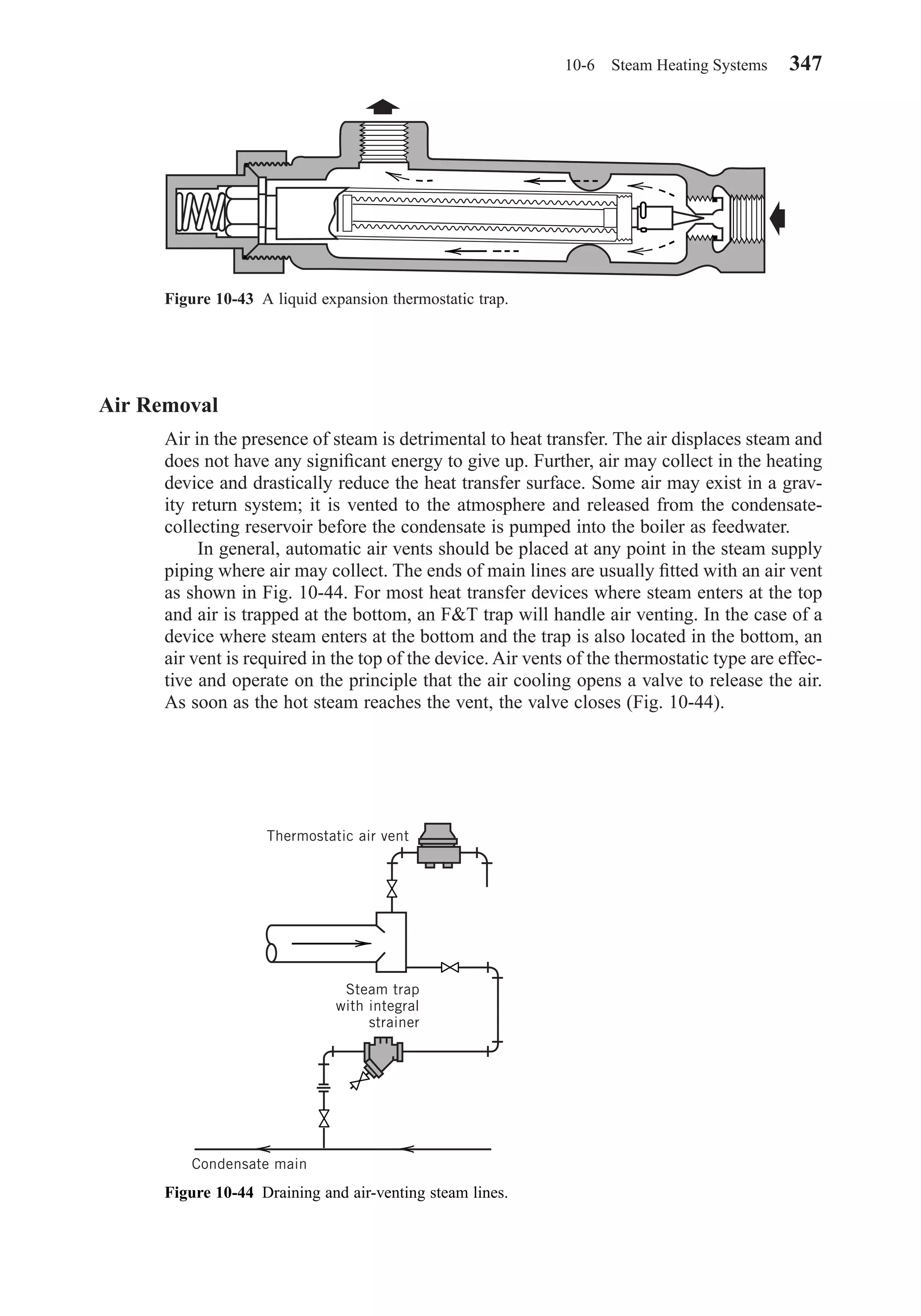
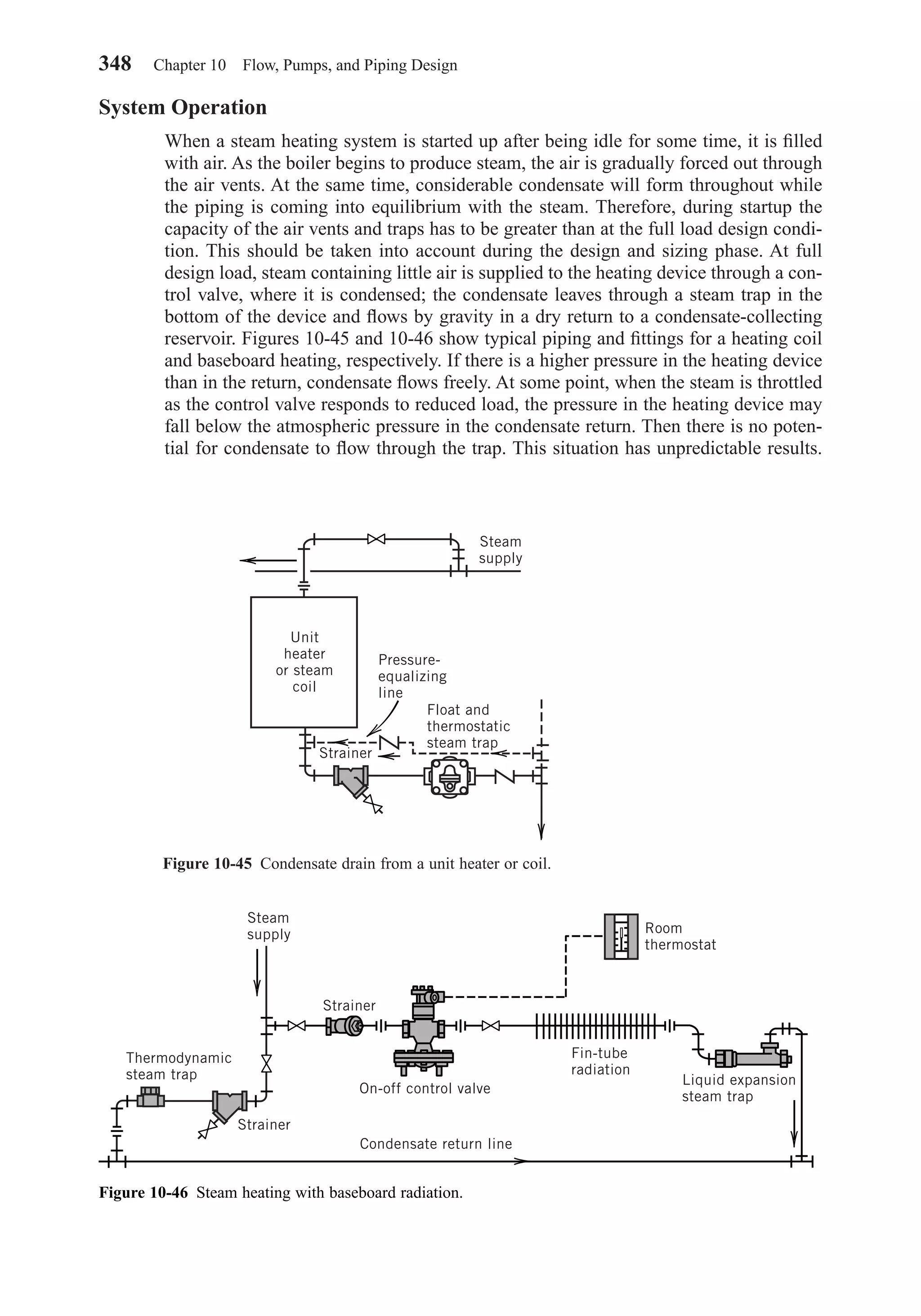
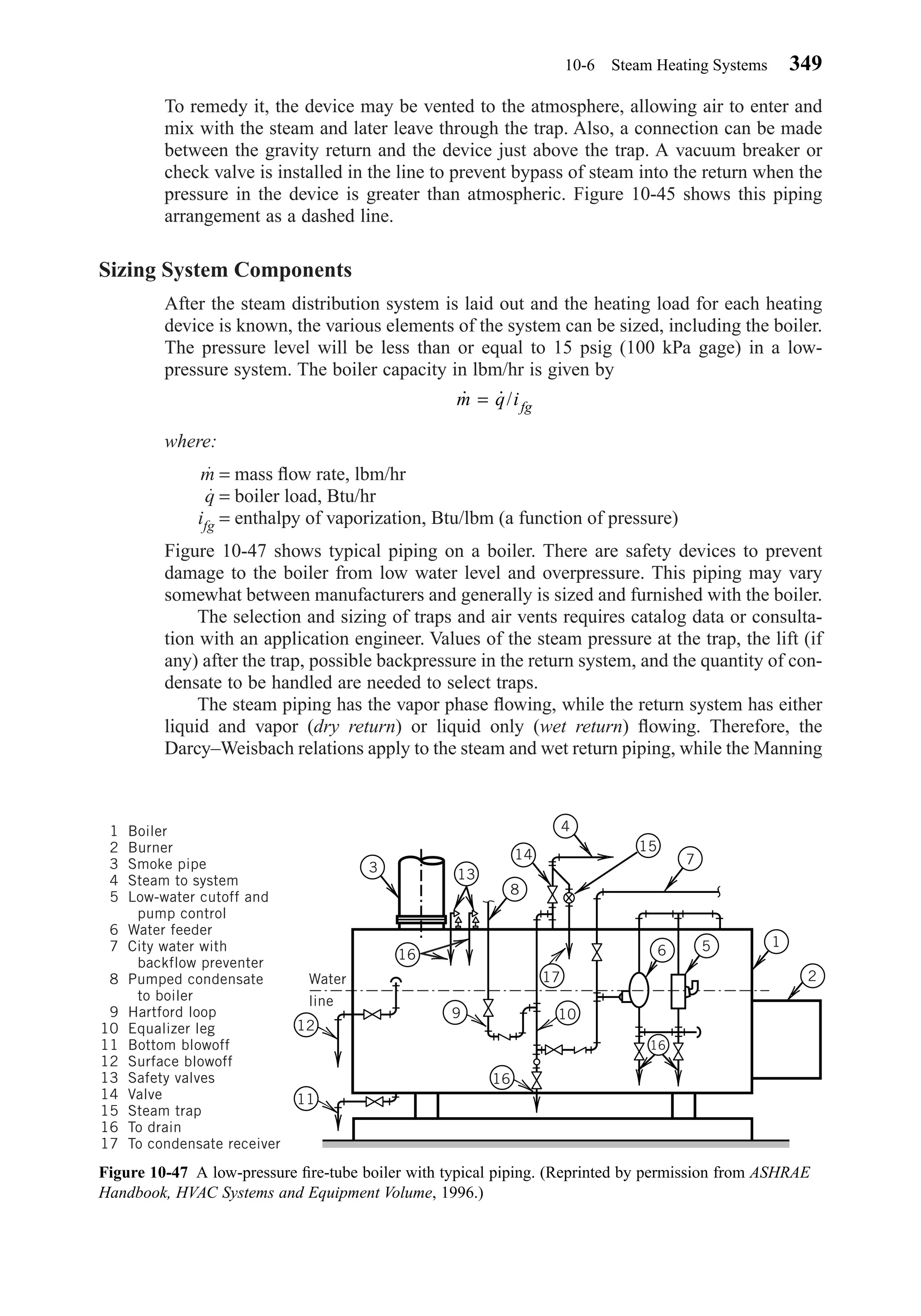
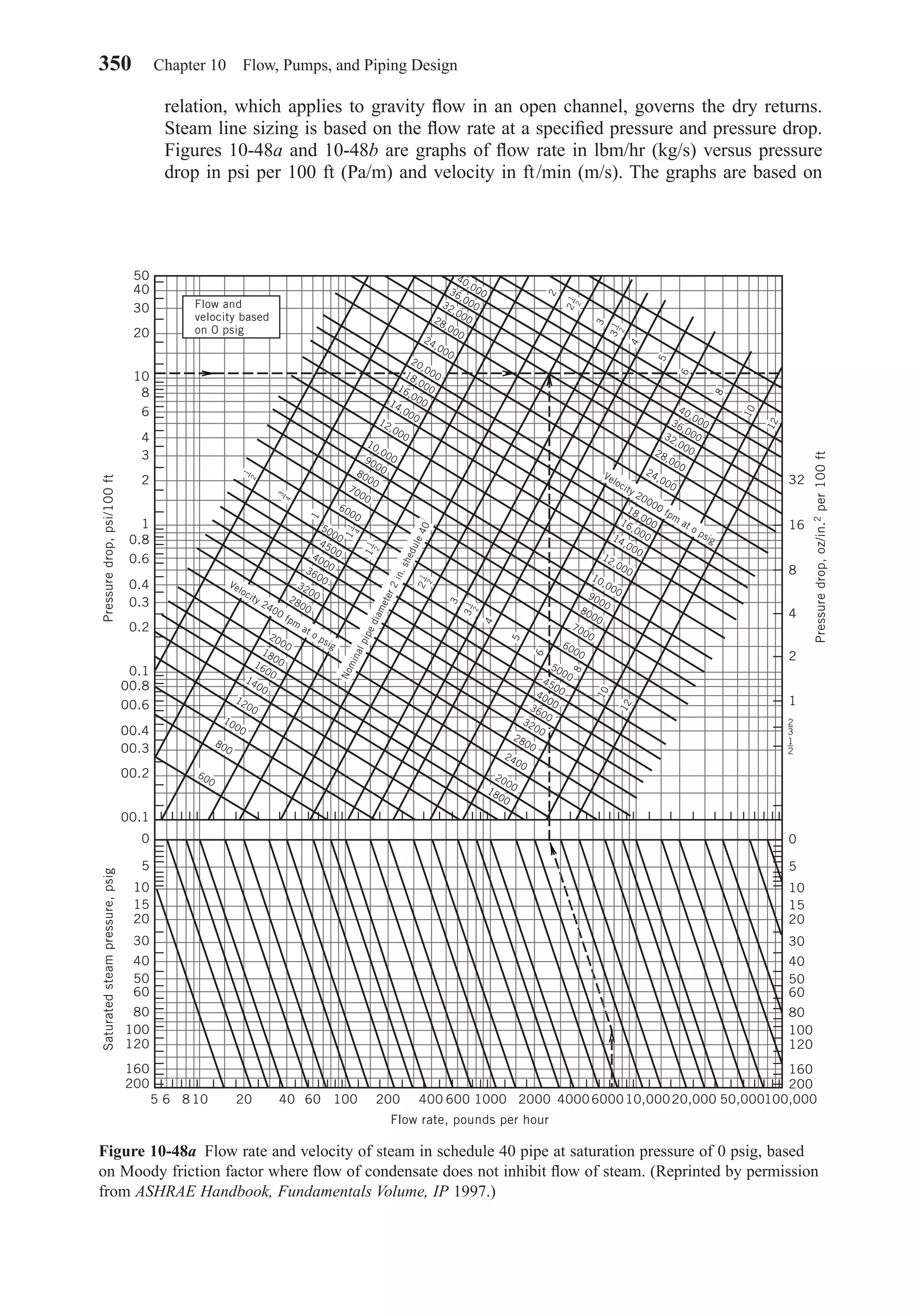
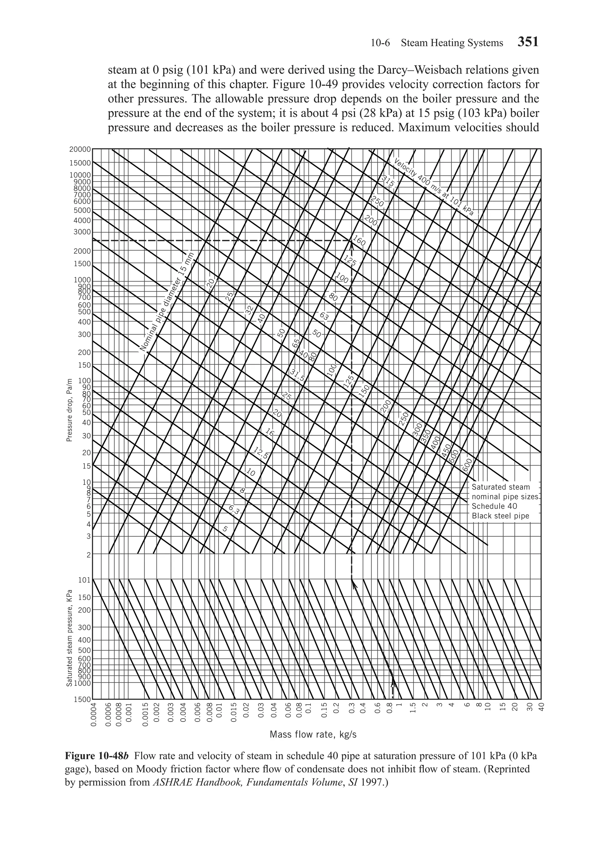
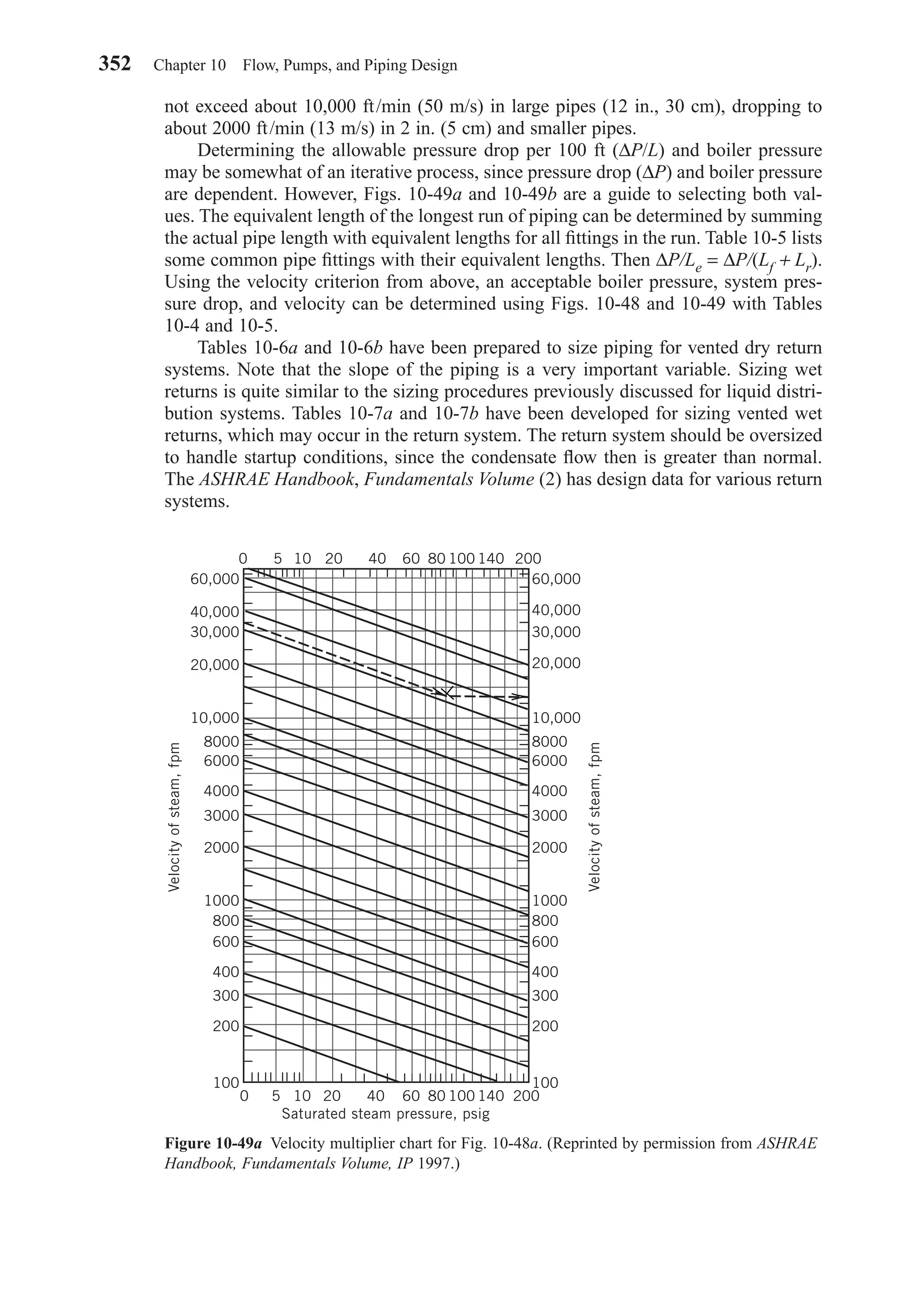
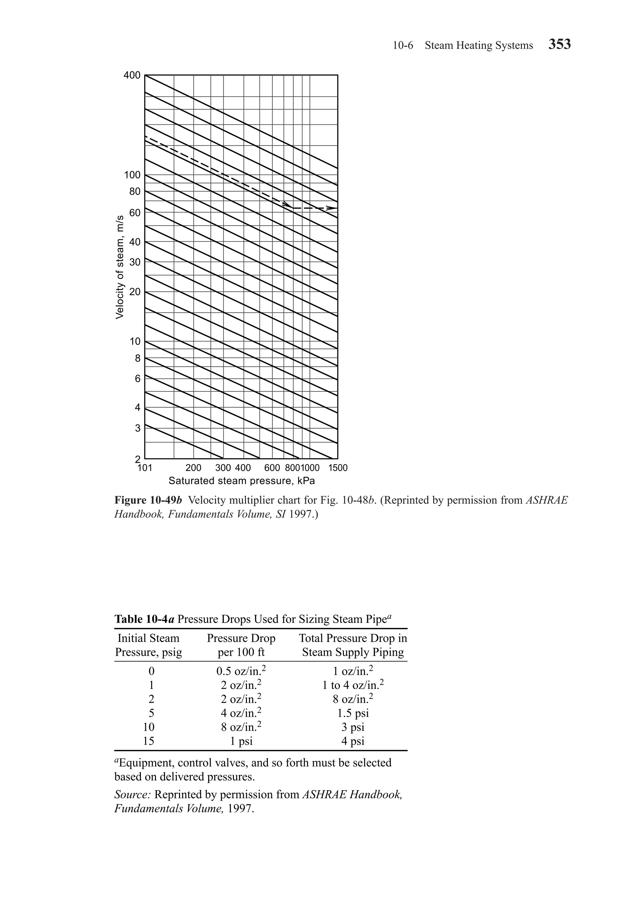
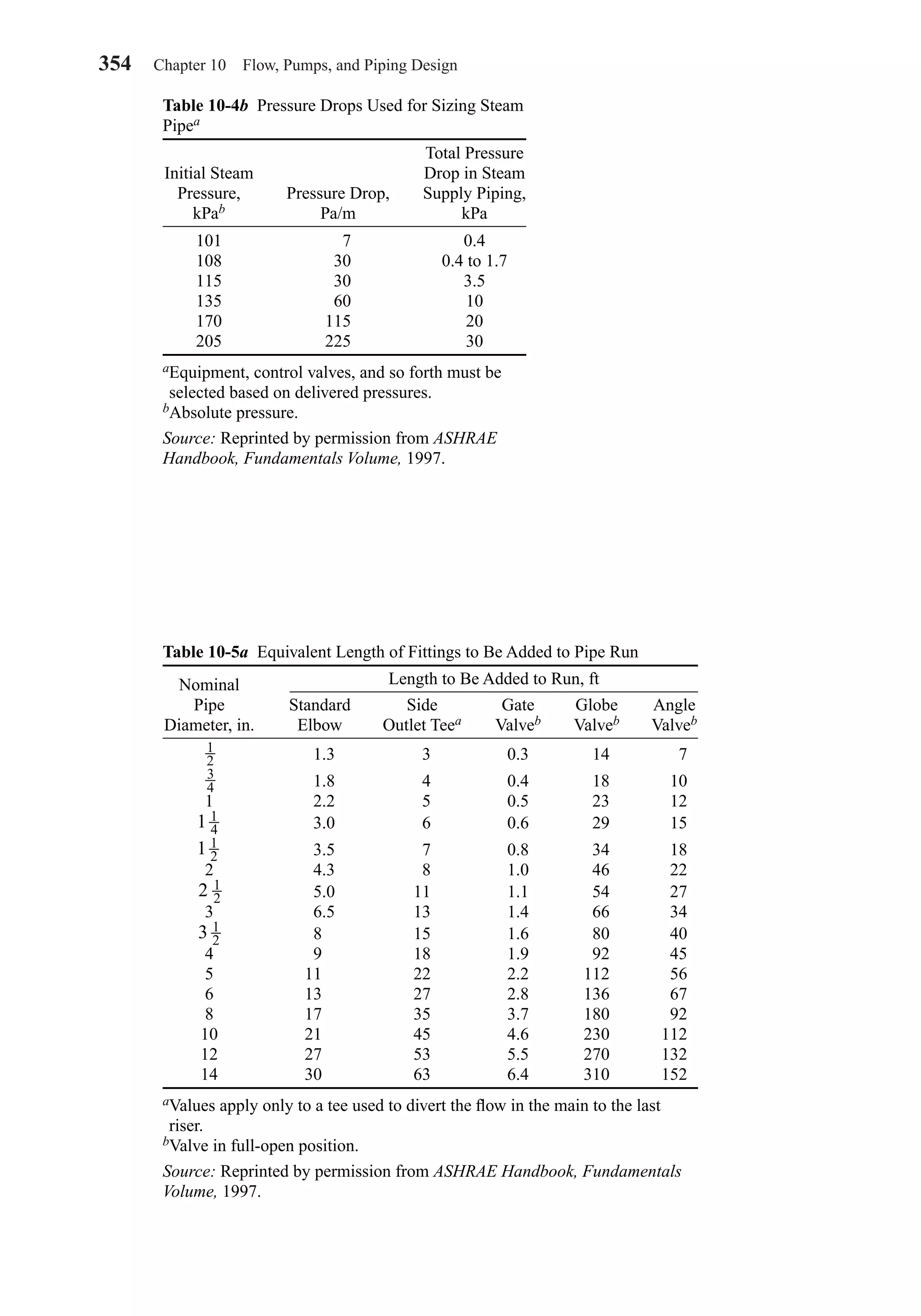
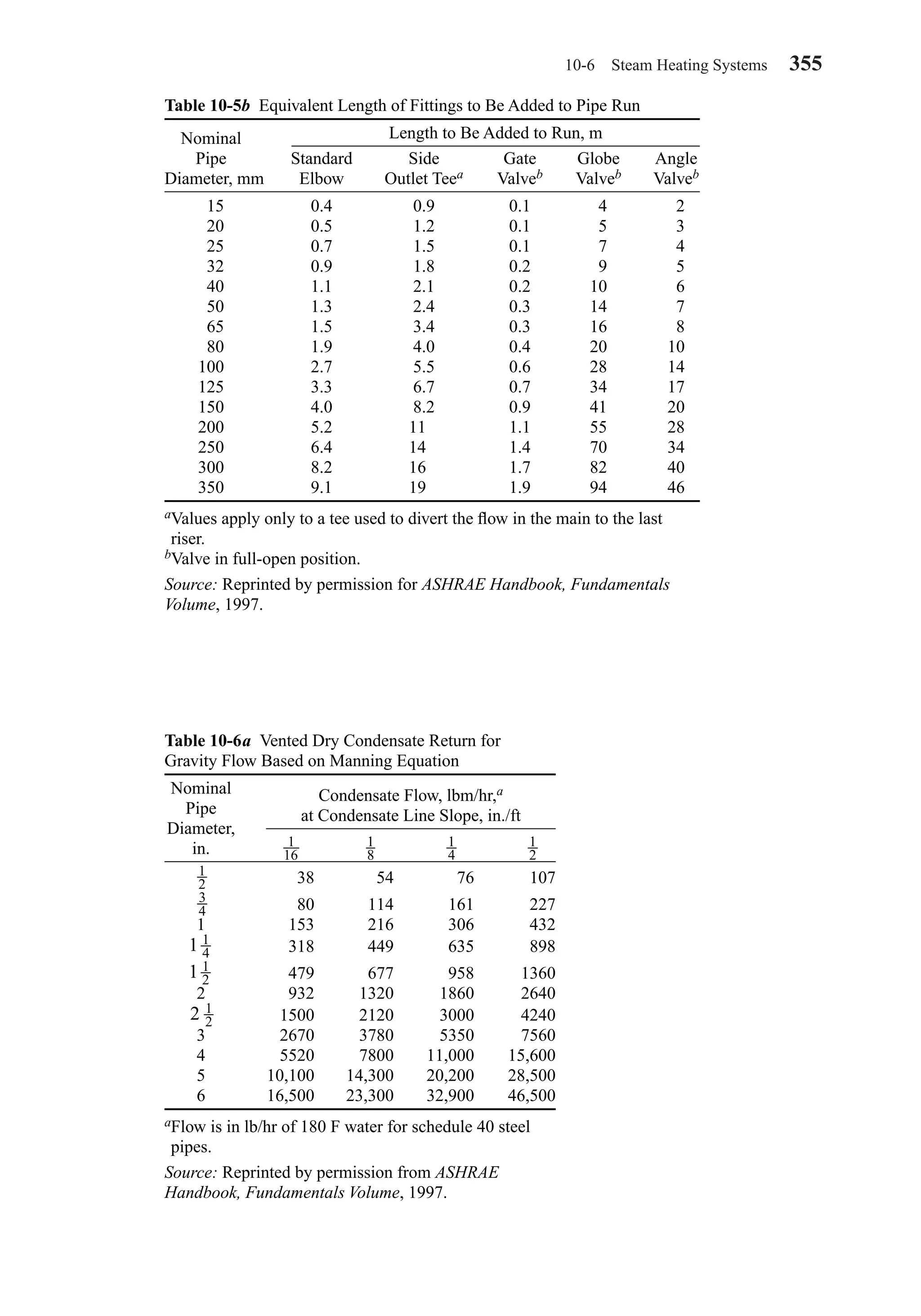
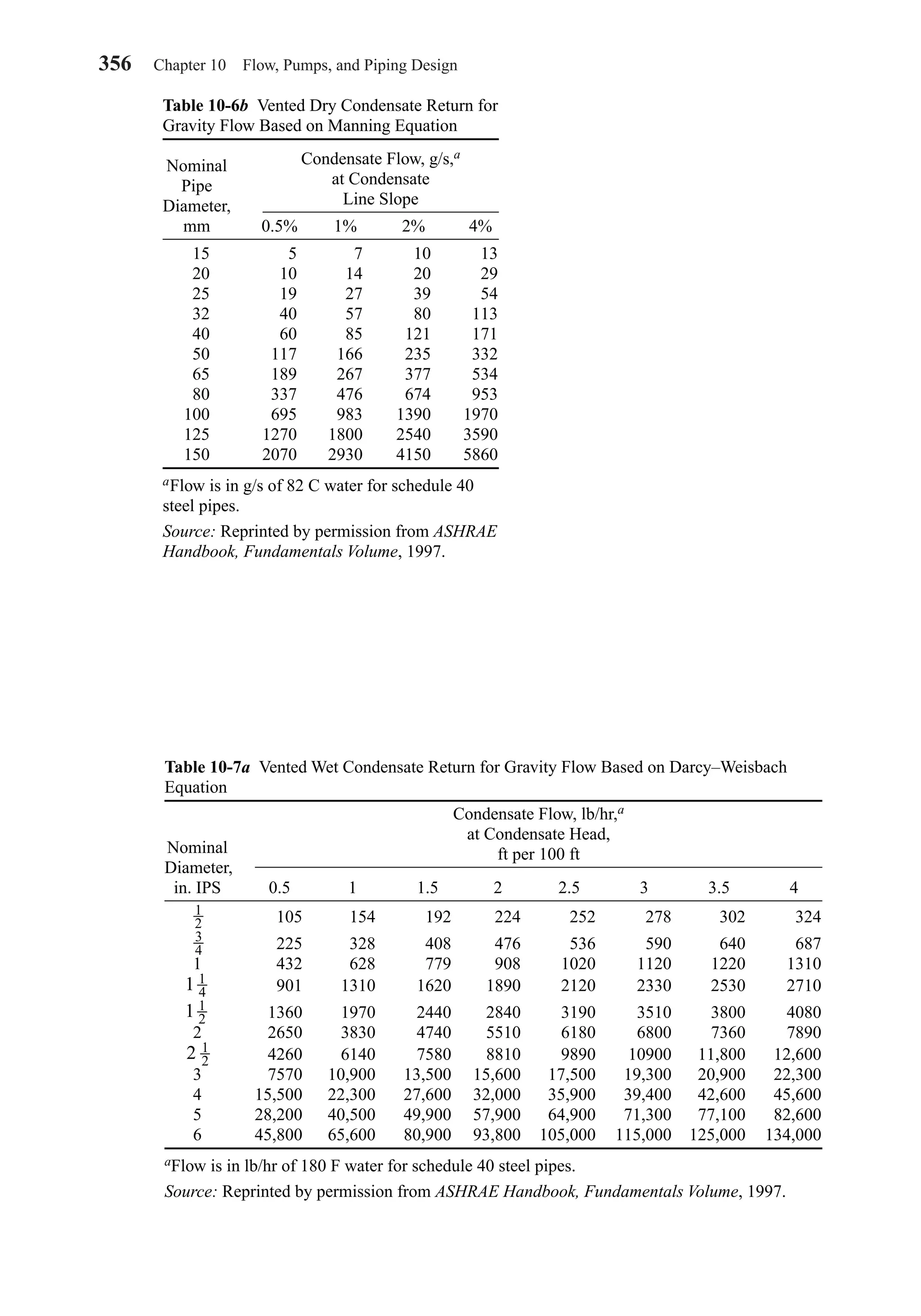
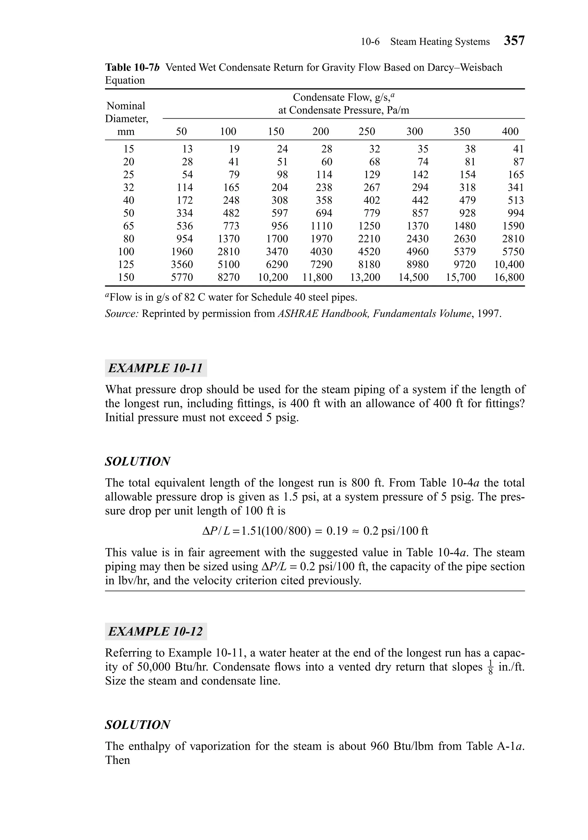
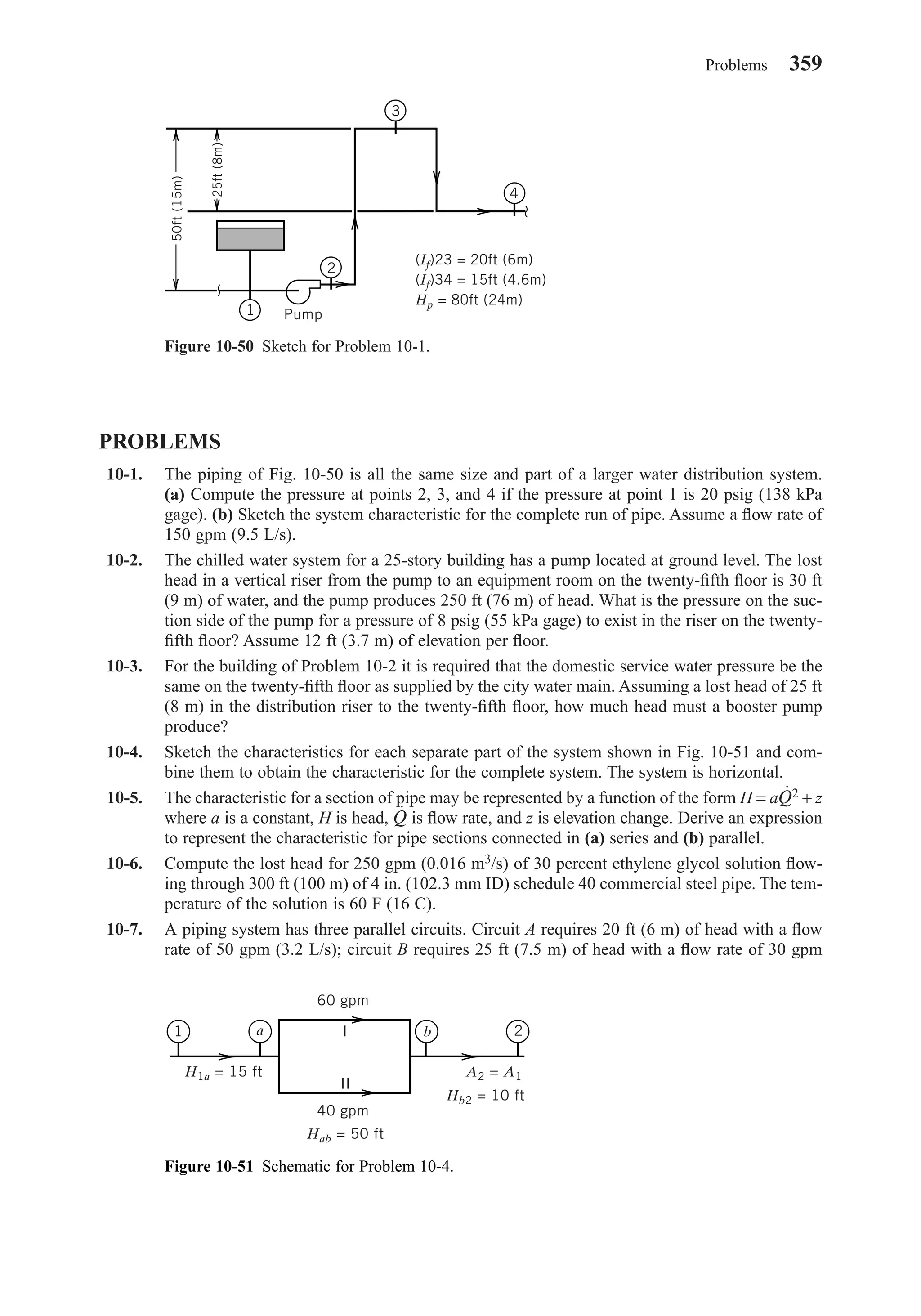

![10-21. Size the piping for the layout shown in Fig. 10-53 and specify the pump requirements. Assume
that all the turns and fittings are as shown on the diagram. The pipe is commercial steel. Table
10-8 gives the required data.
10-22. Size the piping and specify pump requirements for a cooling tower installation similar to that
shown in Fig. 10-18. The volume flow rate of the water is 500 gpm (0.032 m3/s). The piping
is commercial steel. Assume that fittings are as shown. The head loss in the condenser is 20 ft
(6.1 m) of water. Cv for the strainer is 250 gpm/psi [0.00603 m3/(s-kPa)]. The horizontal
Problems 361
Figure 10-52 Sketch for Problem 10-20.
Cooling
tower
Ball
valveStrainer
Condenser
coil
Gate
valve
3m
Figure 10-53 Sketch for Problem 10-21. Lengths are in feet with meters in parentheses.
5 (2) 10 (3)
10 (3)
25 (8)
10 (3)
10 (3) 10 (3)
10 (3)
15 (5)
8 (3) 8 (3) 8 (3)
10 (3)
Typical
3-way valve
Make up
Typical
gate valve
a b c
Chiller
5 (2)
18 (6)
Table 10-8 Data for Problem 10-21
Unit gpm m3/s ft m gpm/psi m3/(s-kPa)
a 30 0.0019 15 5 12 0.000290
b 40 0.0025 12 4 18 0.000434
c 50 0.0032 10 4 24 0.000578
Chiller 120 0.0076 20 10 — —
Head Loss
Flow Rate Coil Cv Value
Chapter10.qxd 6/15/04 2:33 PM Page 361](https://image.slidesharecdn.com/fayec-160521192803/75/Faye-c-mc_quiston_-_jerald_d-_parker_-_jeffrey_d-379-2048.jpg)
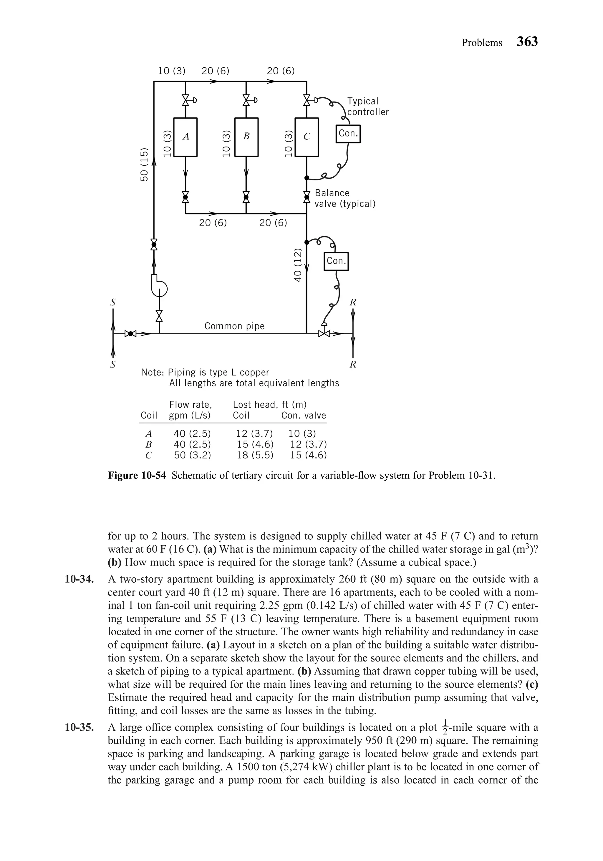
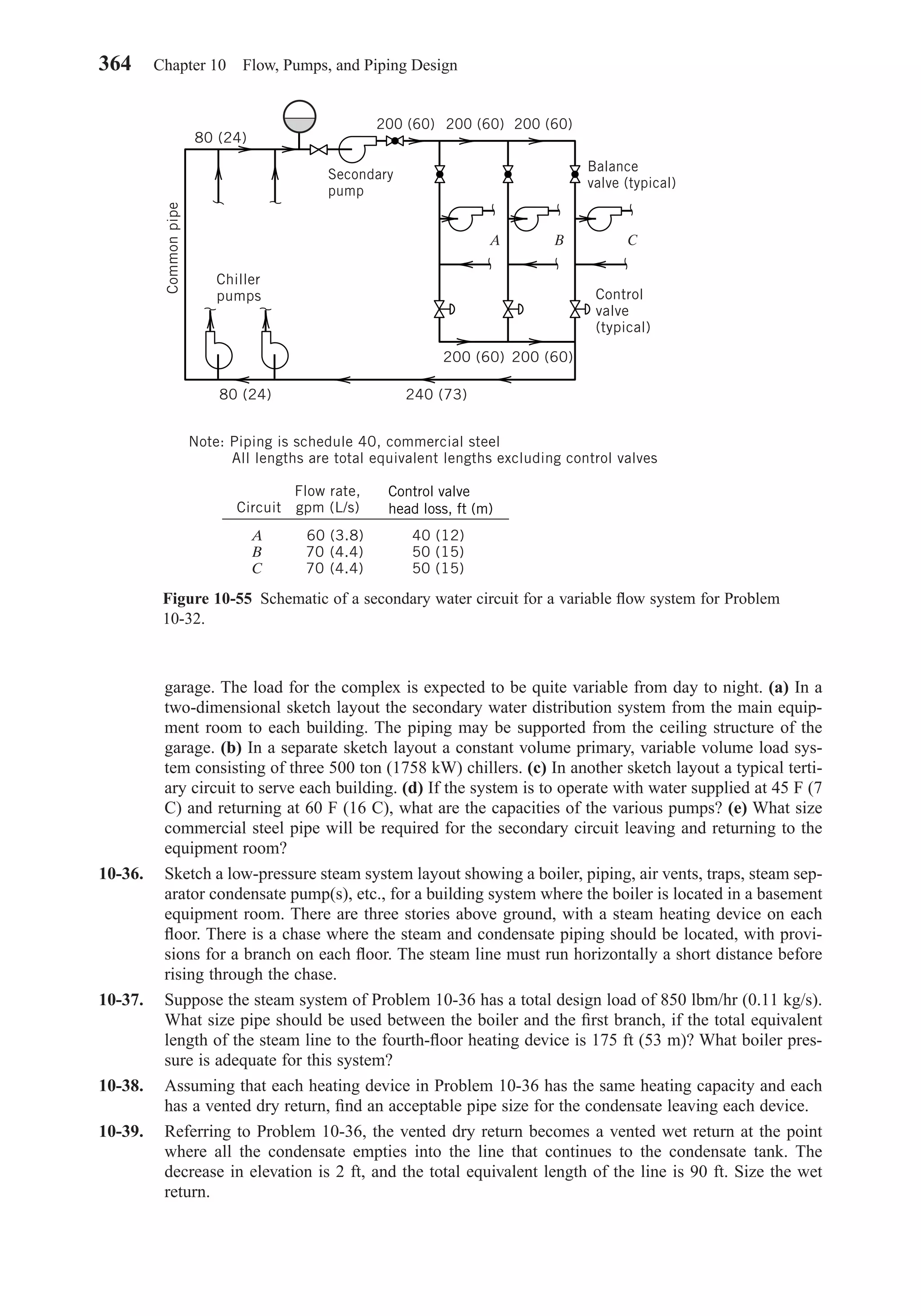
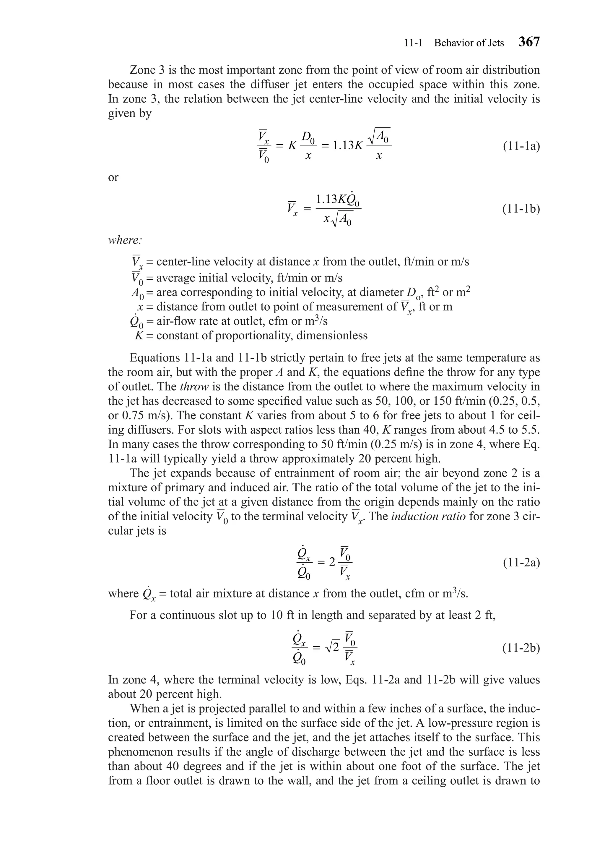
![the ceiling. This surface effect increases the throw for all types of outlets and
decreases the drop for horizontal jets. Buoyant forces cause the jet to rise when the
air is warm and drop when cool, relative to room temperature. These conditions result
in shorter throws for jet velocities less than 150 ft/min (0.76 m/s). The following gen-
eral statements may be made concerning the characteristics of air jets:
1. Surface effect increases the throw and decreases the drop compared to free
space conditions.
2. Increased surface effect may be obtained by moving the outlet away from the
surface somewhat so that the jet spreads over the surface after impact.
3. Increased surface effect may be obtained by spreading the jet when it is
discharged.
4. Spreading the airstream reduces the throw and drop.
5. Drop primarily depends on the quantity of air and only partially on the outlet size
or velocity. Thus the use of more outlets with less air per outlet reduces drop.
Room Air Motion
Room air near the jet is entrained and must then be replaced by other room air. The
room air moves toward the supply and sets all the room air into motion. Whenever the
average room air velocity is less than about 50 ft/min (0.25 m/s), buoyancy effects
may be significant. In general, about 8 to 10 air changes per hour are required to pre-
vent stagnant regions (velocity less than 15 ft/min [0.08 m/s]). However, stagnant
regions are not necessarily a serious condition. The general approach is to supply air
in such a way that the high-velocity air from the outlet does not enter the occupied
space. The region within 1 ft of the wall and above about 6 ft from the floor is out of
the occupied space for practical purposes.
Figure 11-1 shows velocity envelopes for a high sidewall outlet. Equation 11-1a
may be used to estimate the throw for the terminal velocities shown. In order to inter-
pret the air motion shown in terms of comfort, it is necessary to estimate the local air
temperatures corresponding to the terminal velocities. The relationship between the
center-line velocities and the temperature differences is given approximately by (2)
(11-3)∆ ∆t t
V
Vx o
x
= 0 8
0
.
368 Chapter 11 Space Air Diffusion
Figure 11-1 Jet and room air velocities and temperatures for V0 = 1000 ft/min and ∆to = −20 F.
50 fpm
tx = –0.8∆
100 fpm
tx = –1.6∆
200 fpm
tx = –3.2∆
Room velocity < 50 fpm
tx ≈ 0∆
Chapter11.qxd 6/15/04 2:37 PM Page 368](https://image.slidesharecdn.com/fayec-160521192803/75/Faye-c-mc_quiston_-_jerald_d-_parker_-_jeffrey_d-386-2048.jpg)
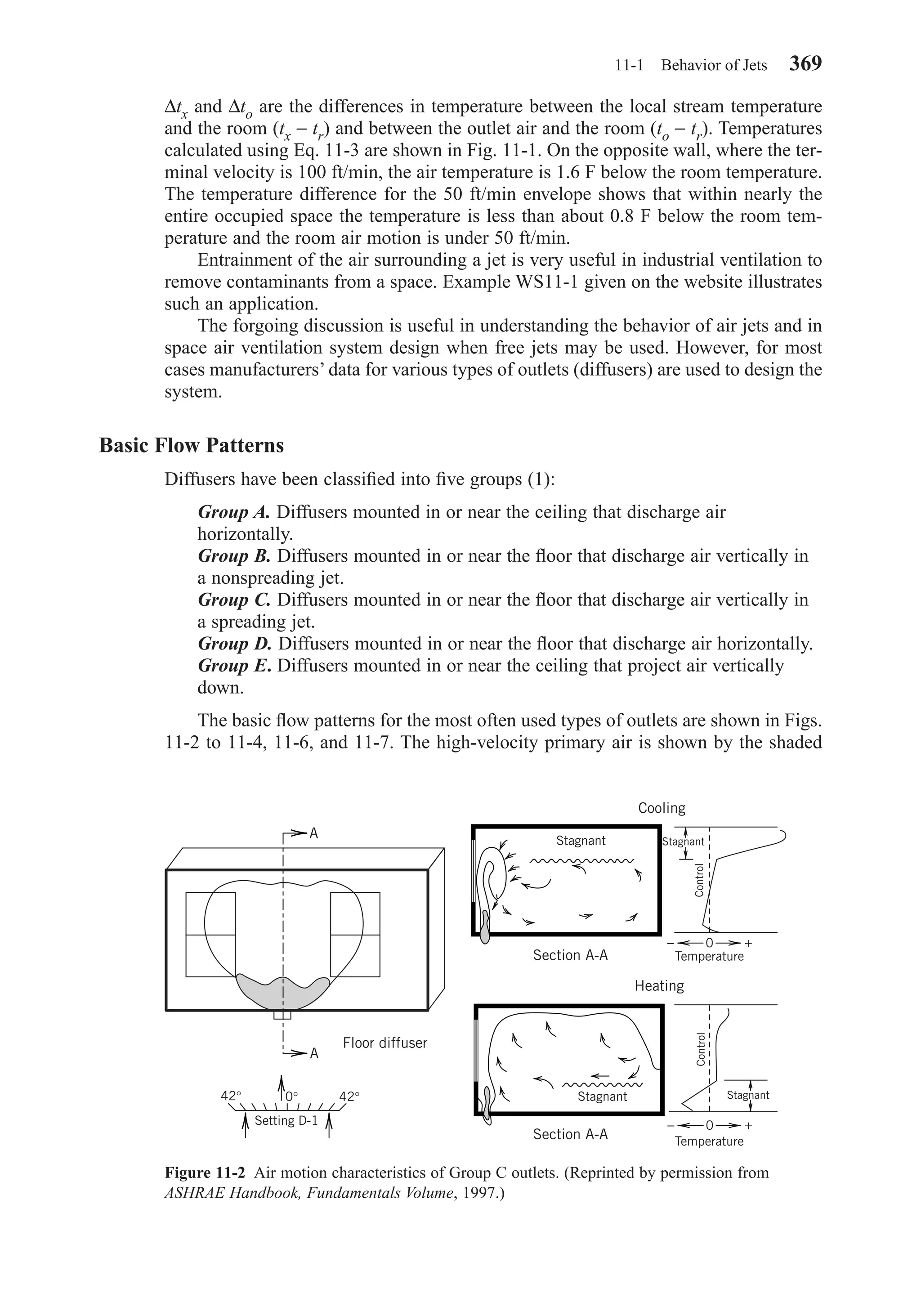
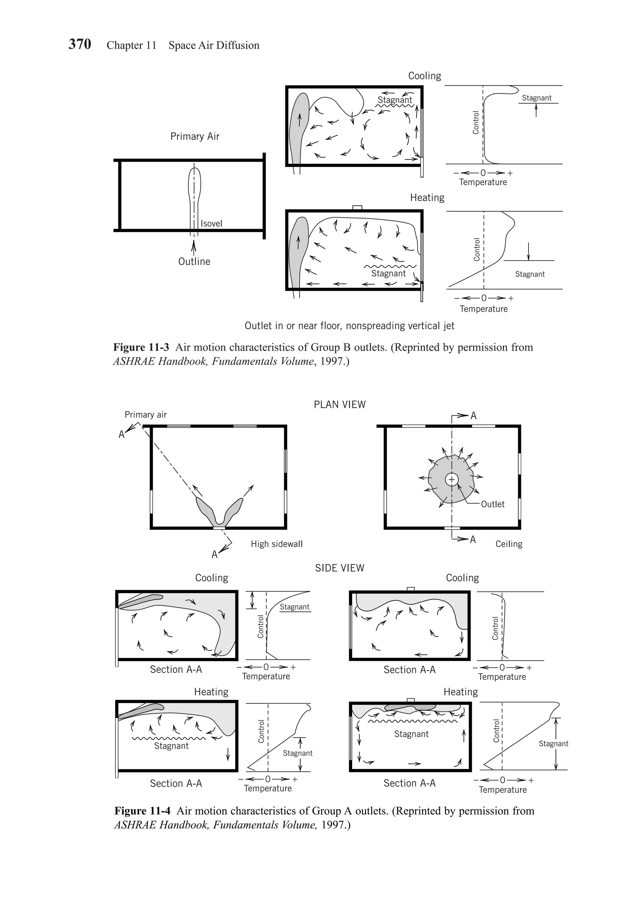
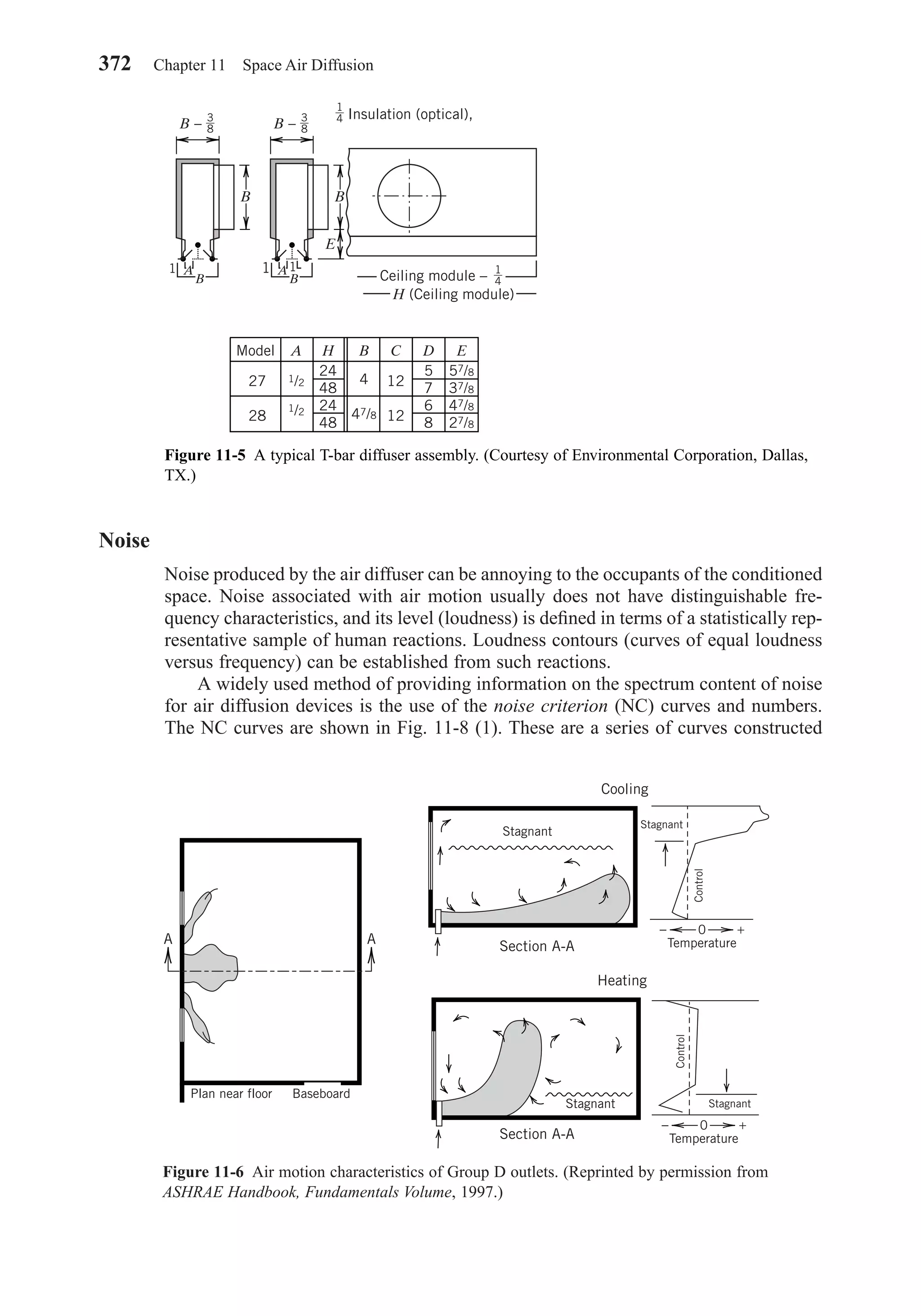
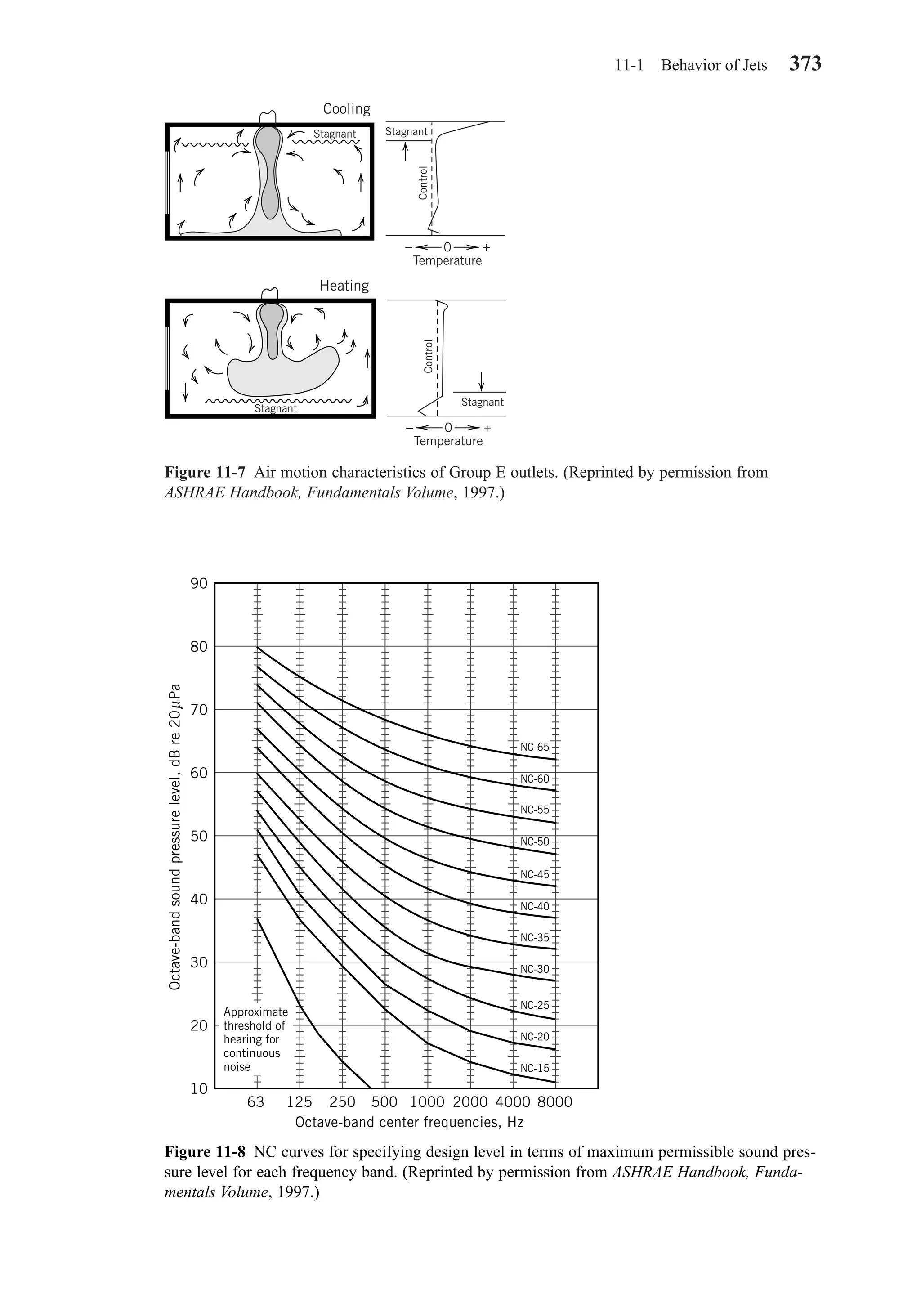
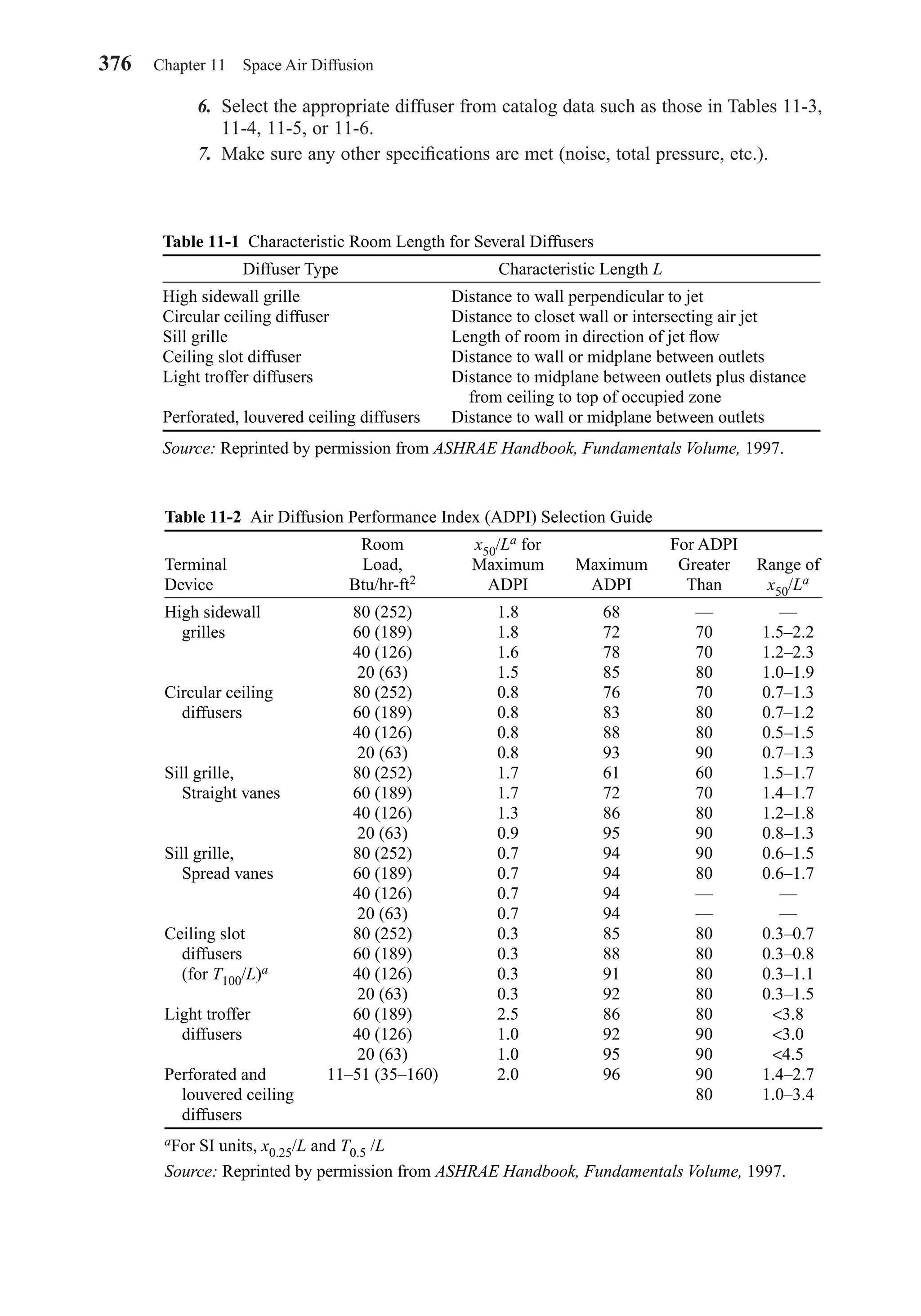
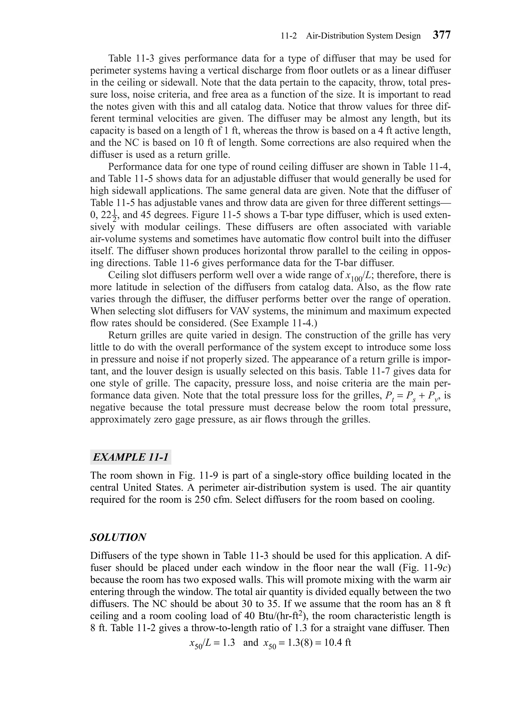
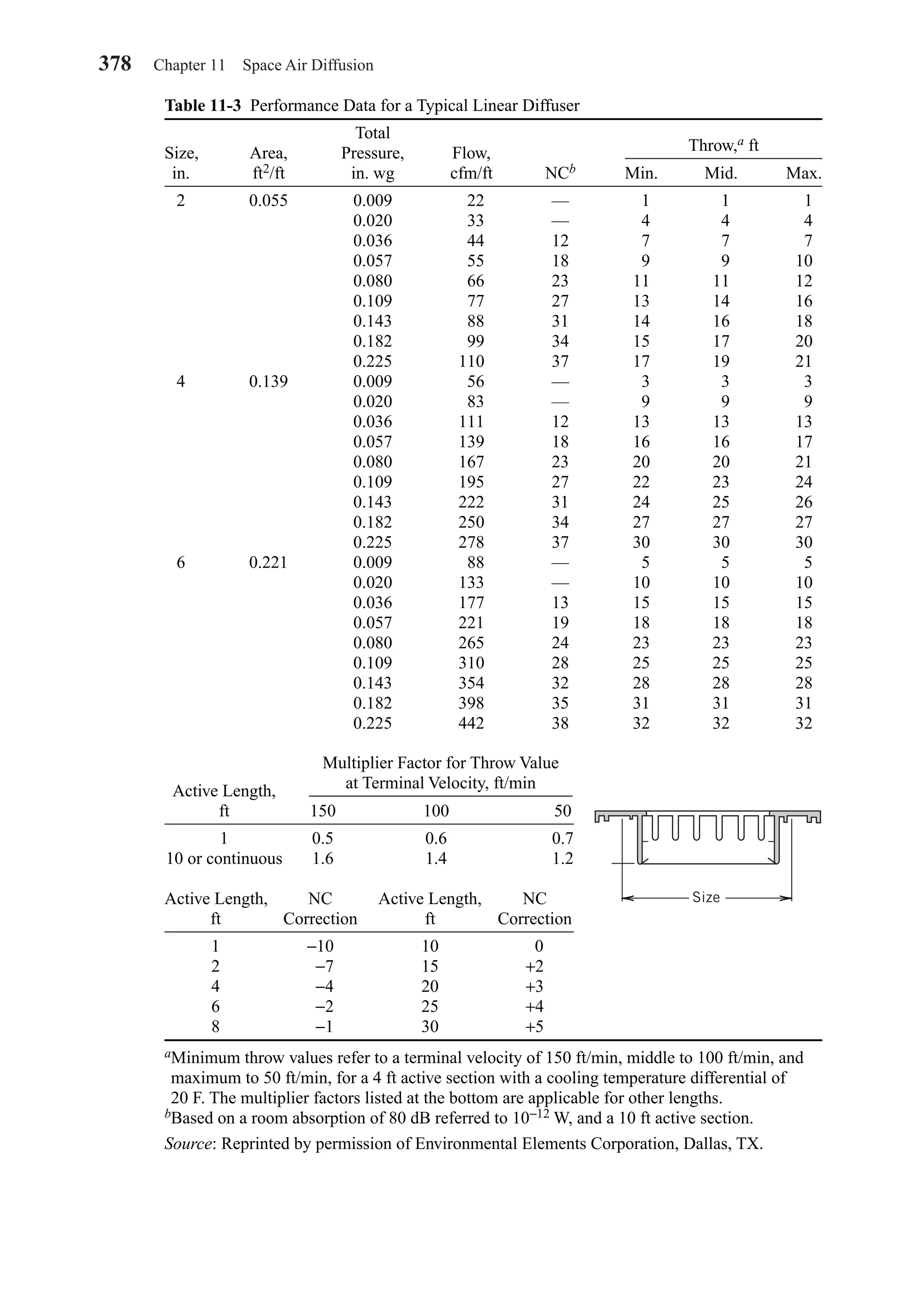
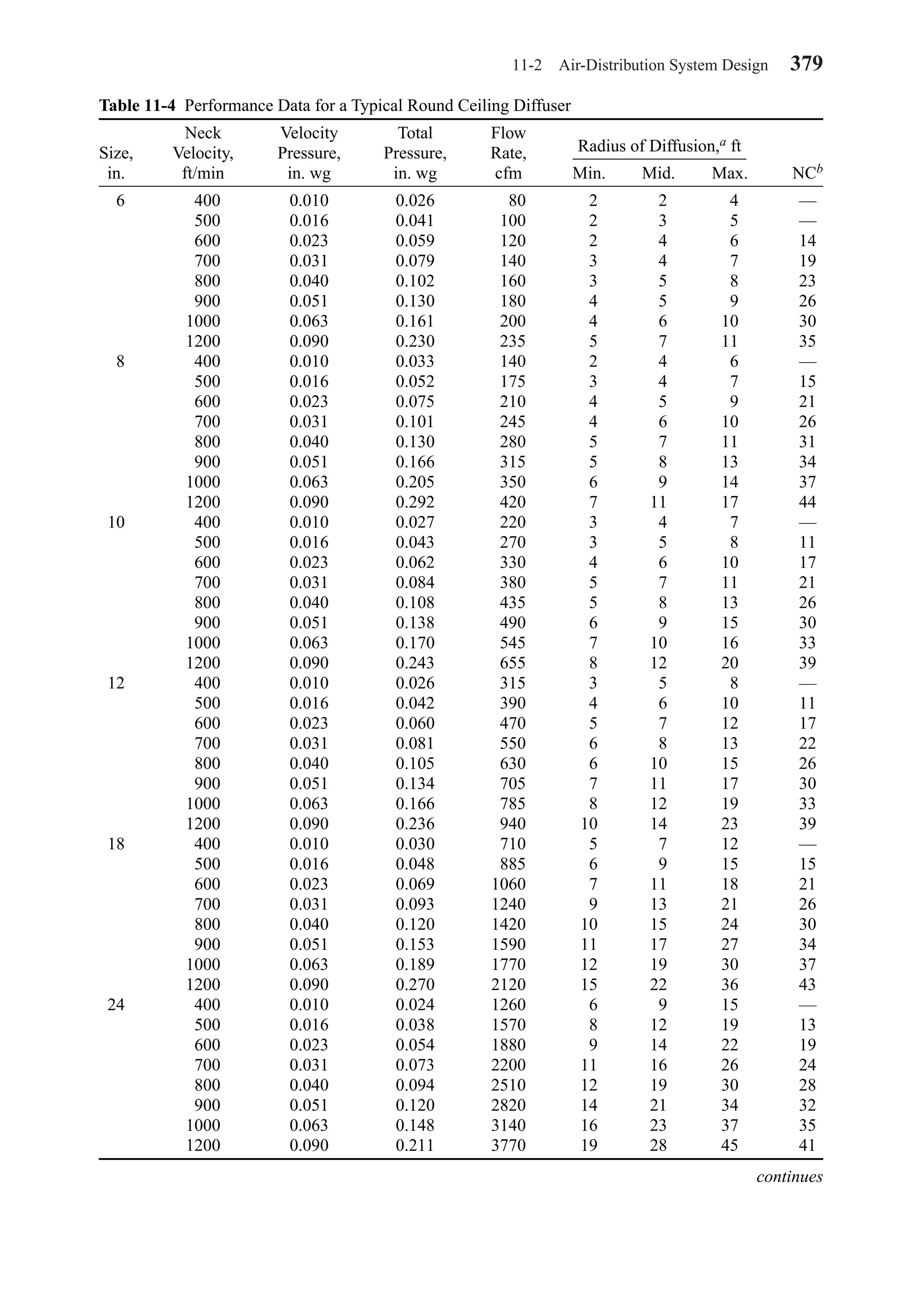
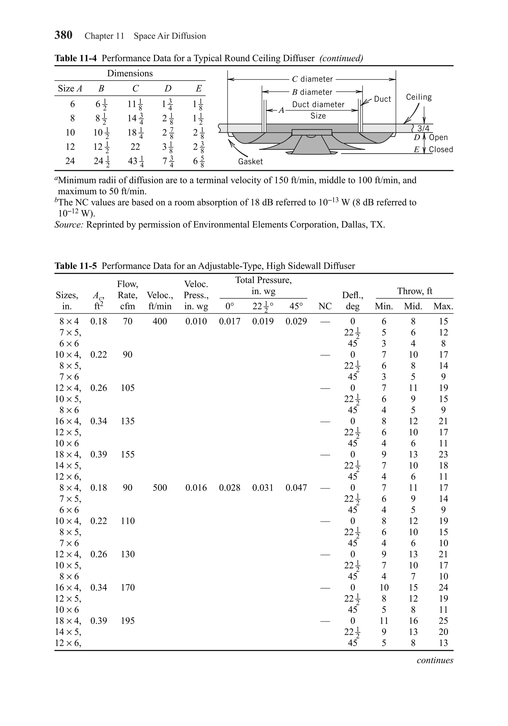
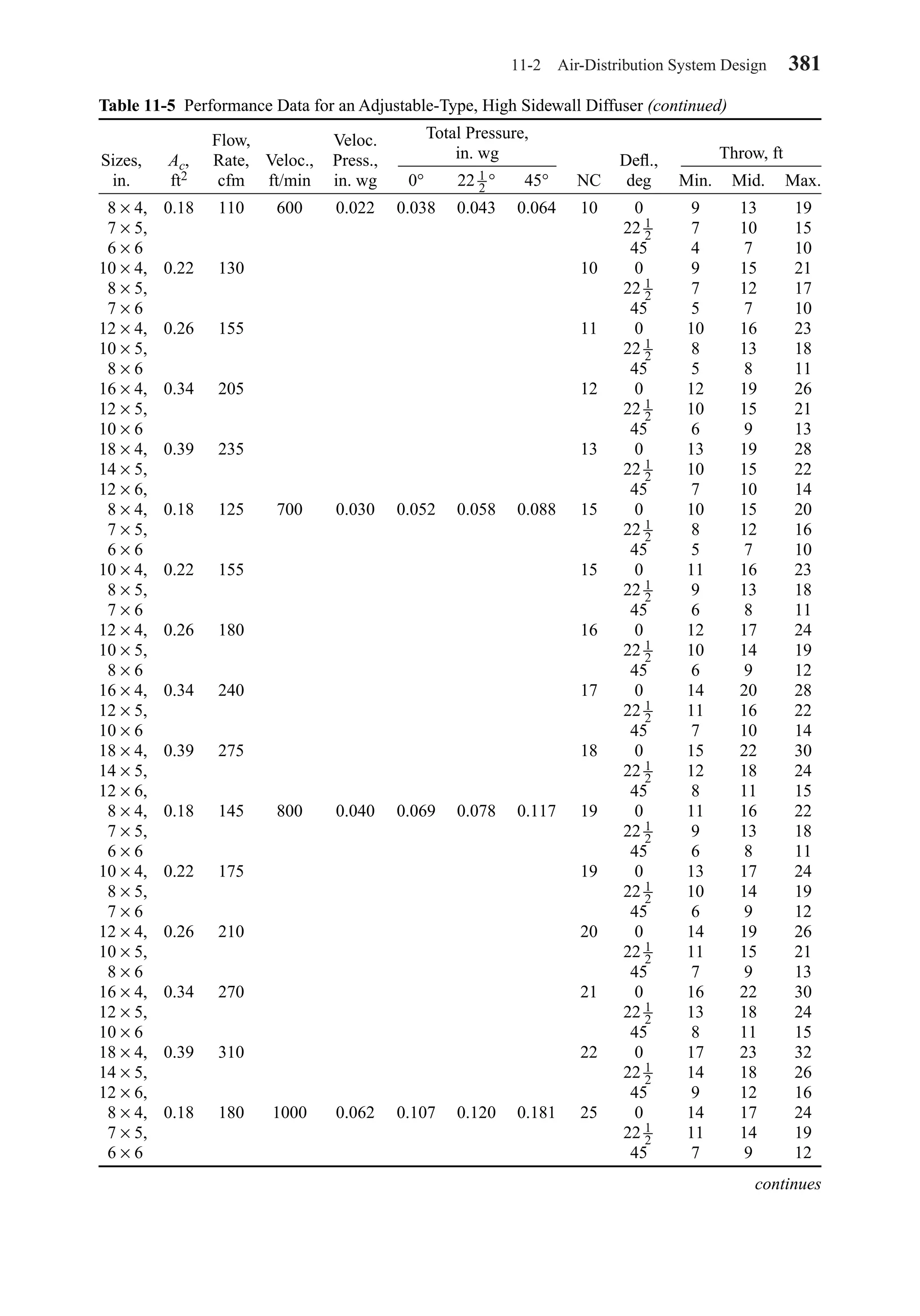
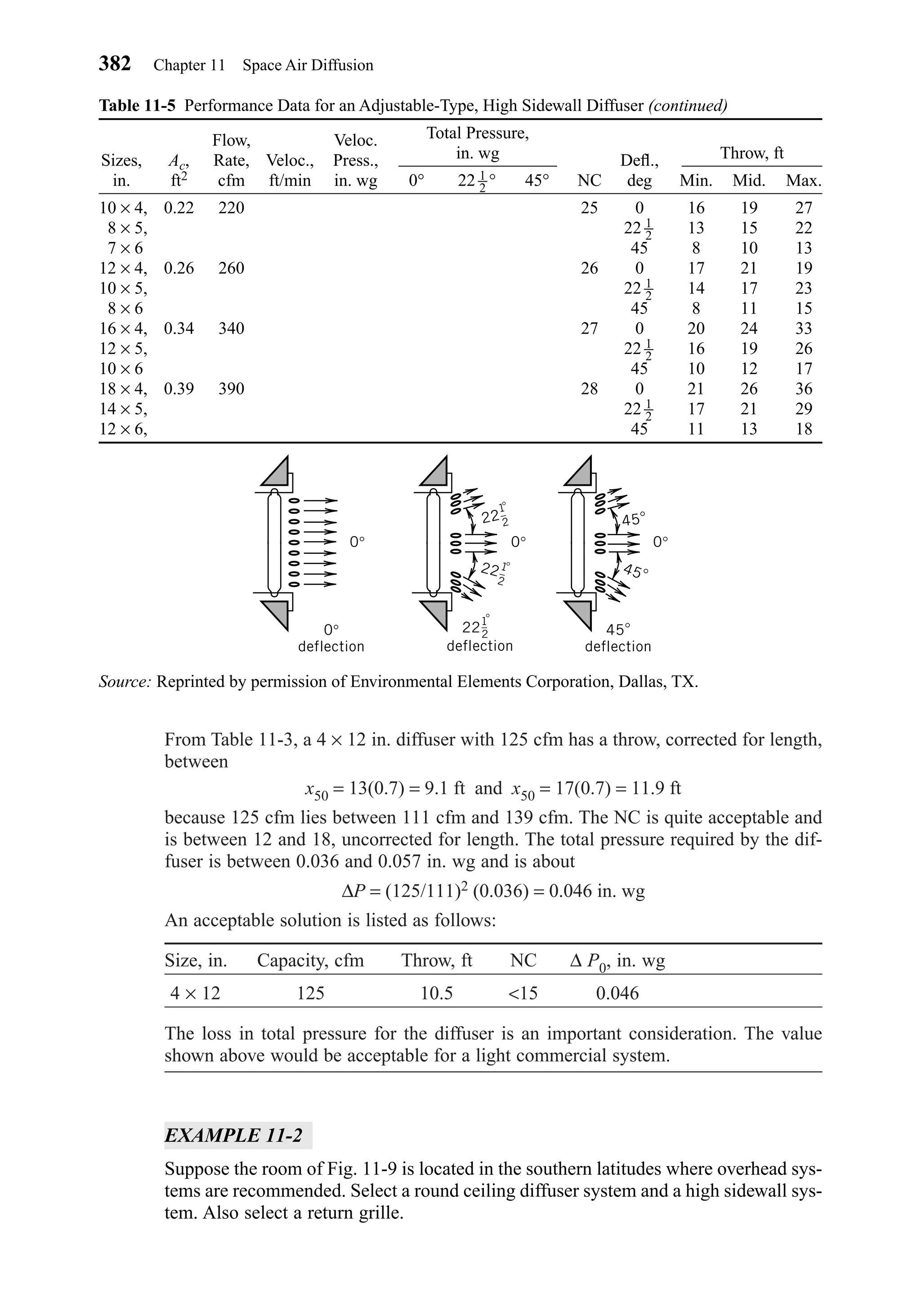
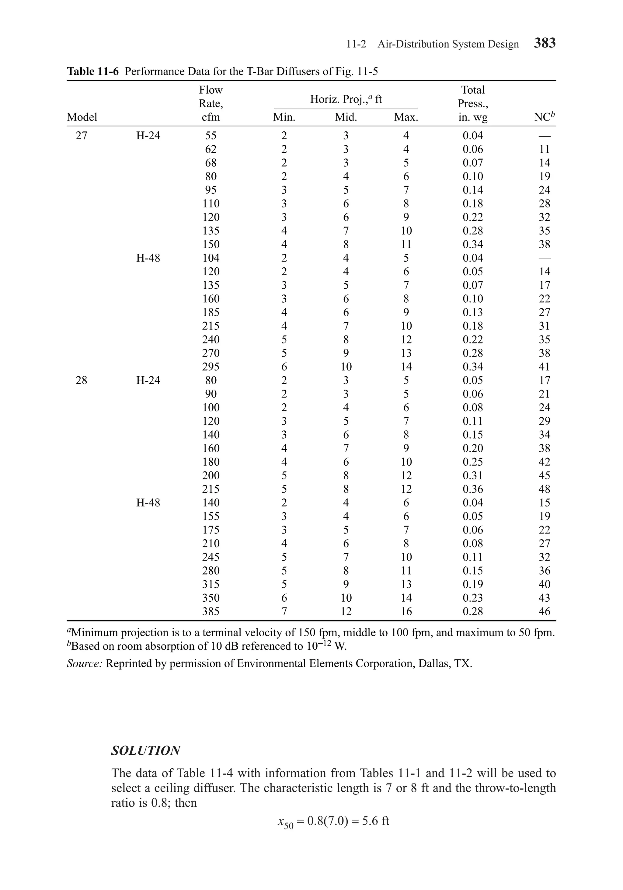
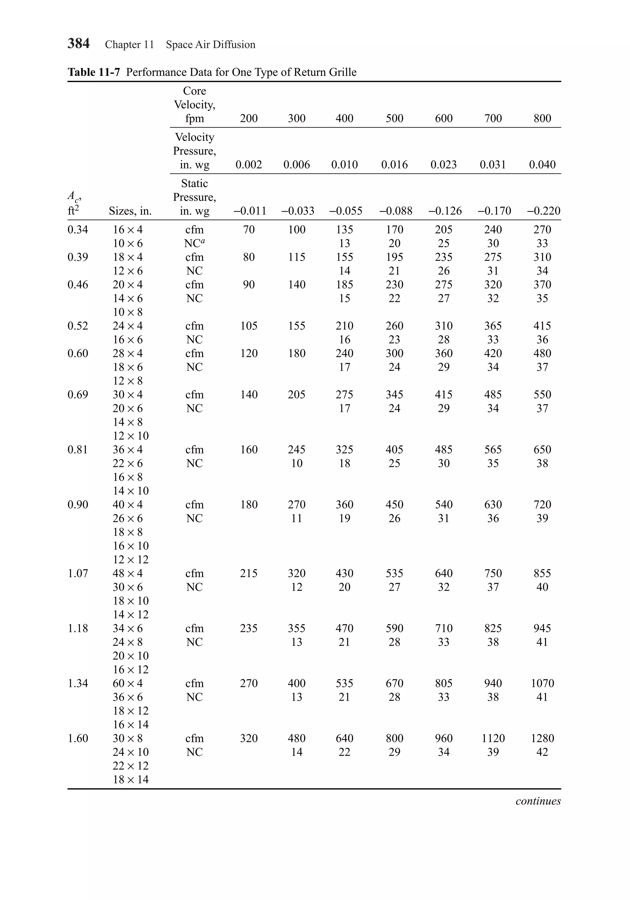
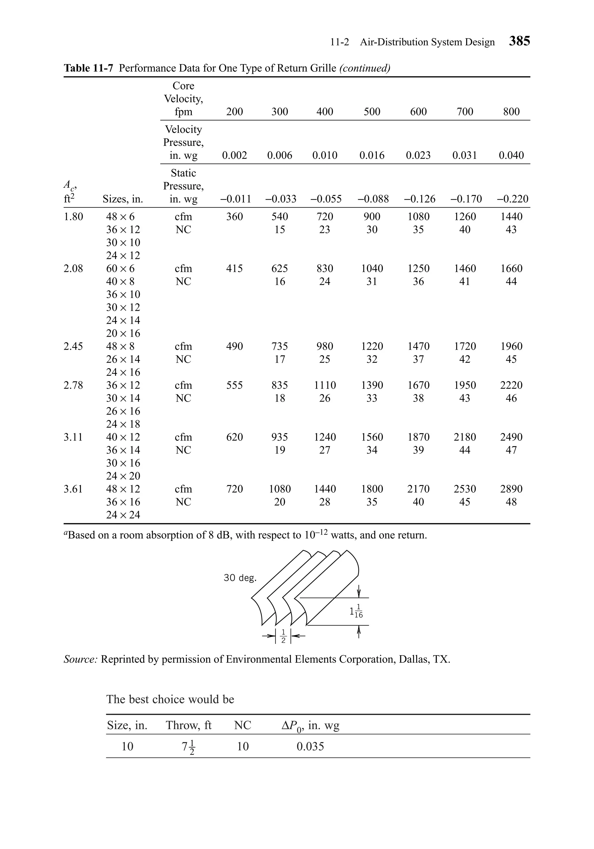
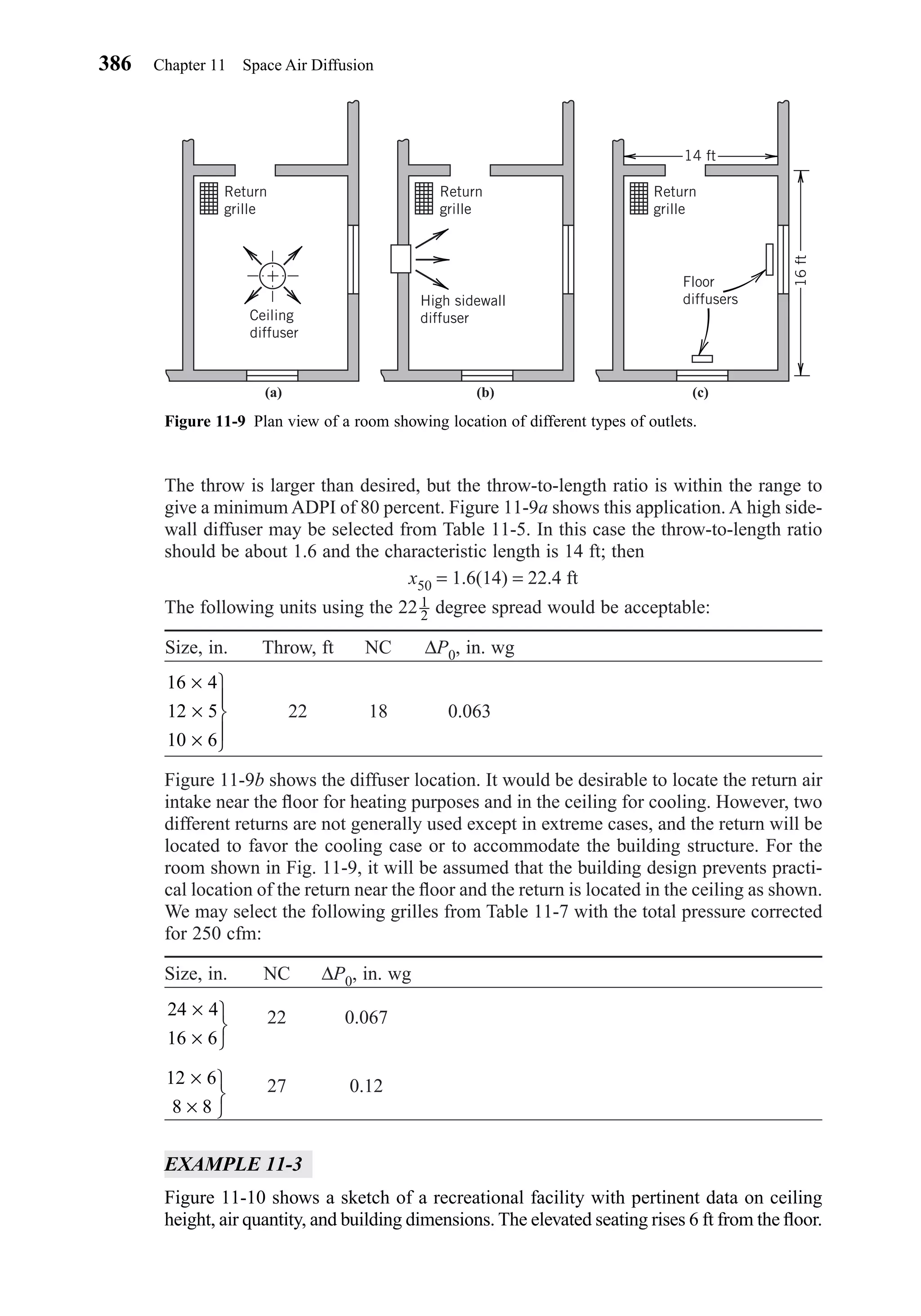
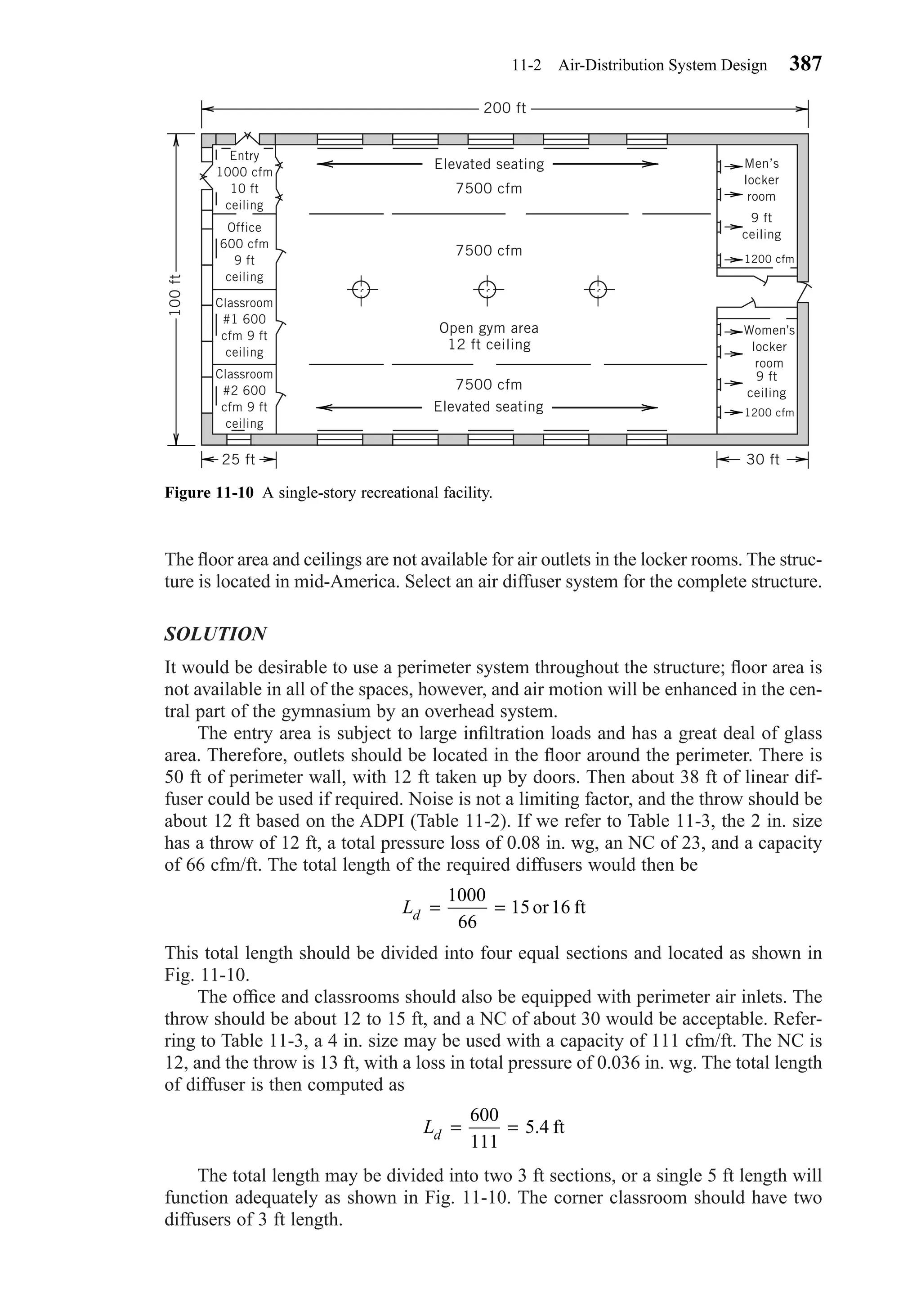
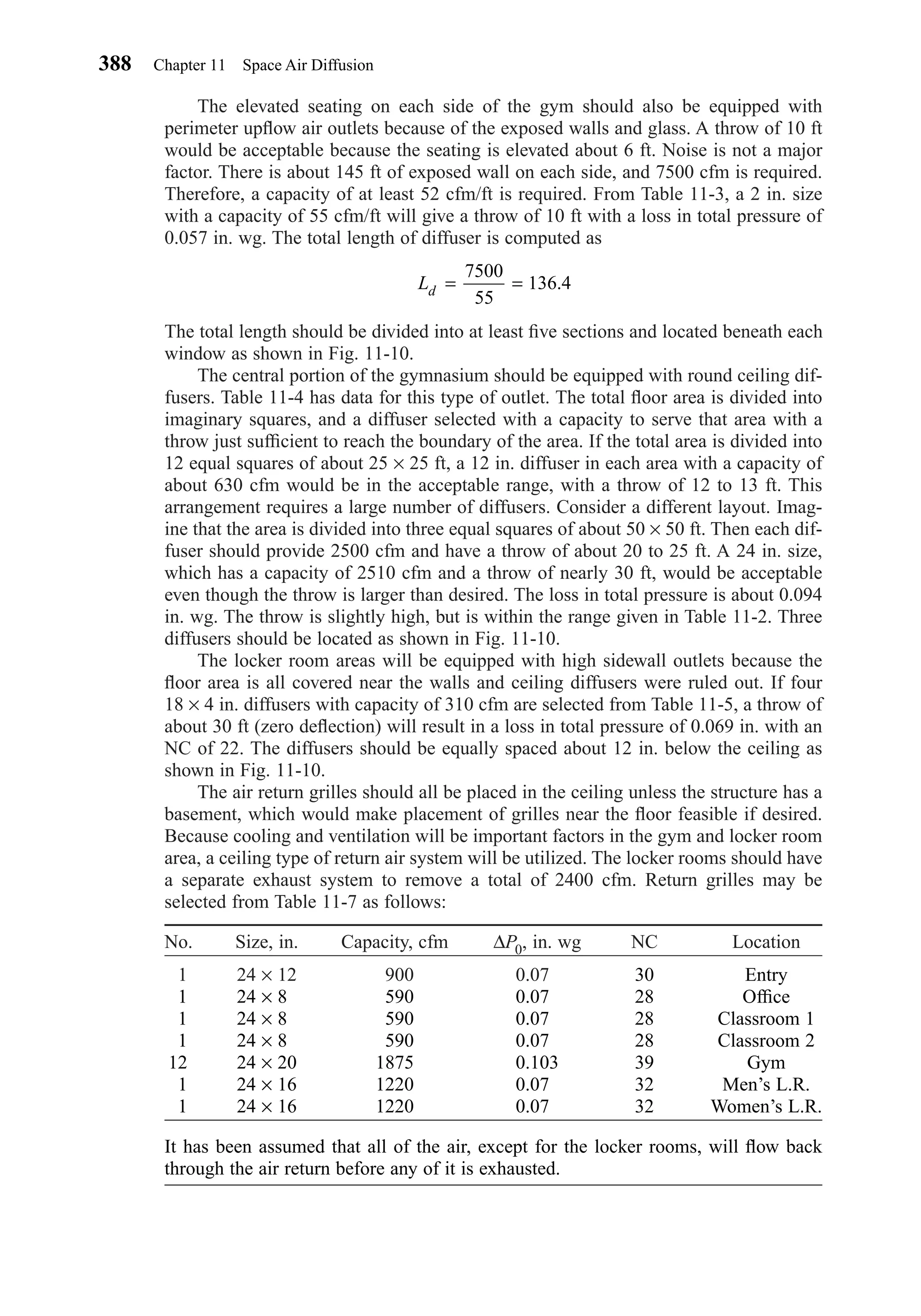
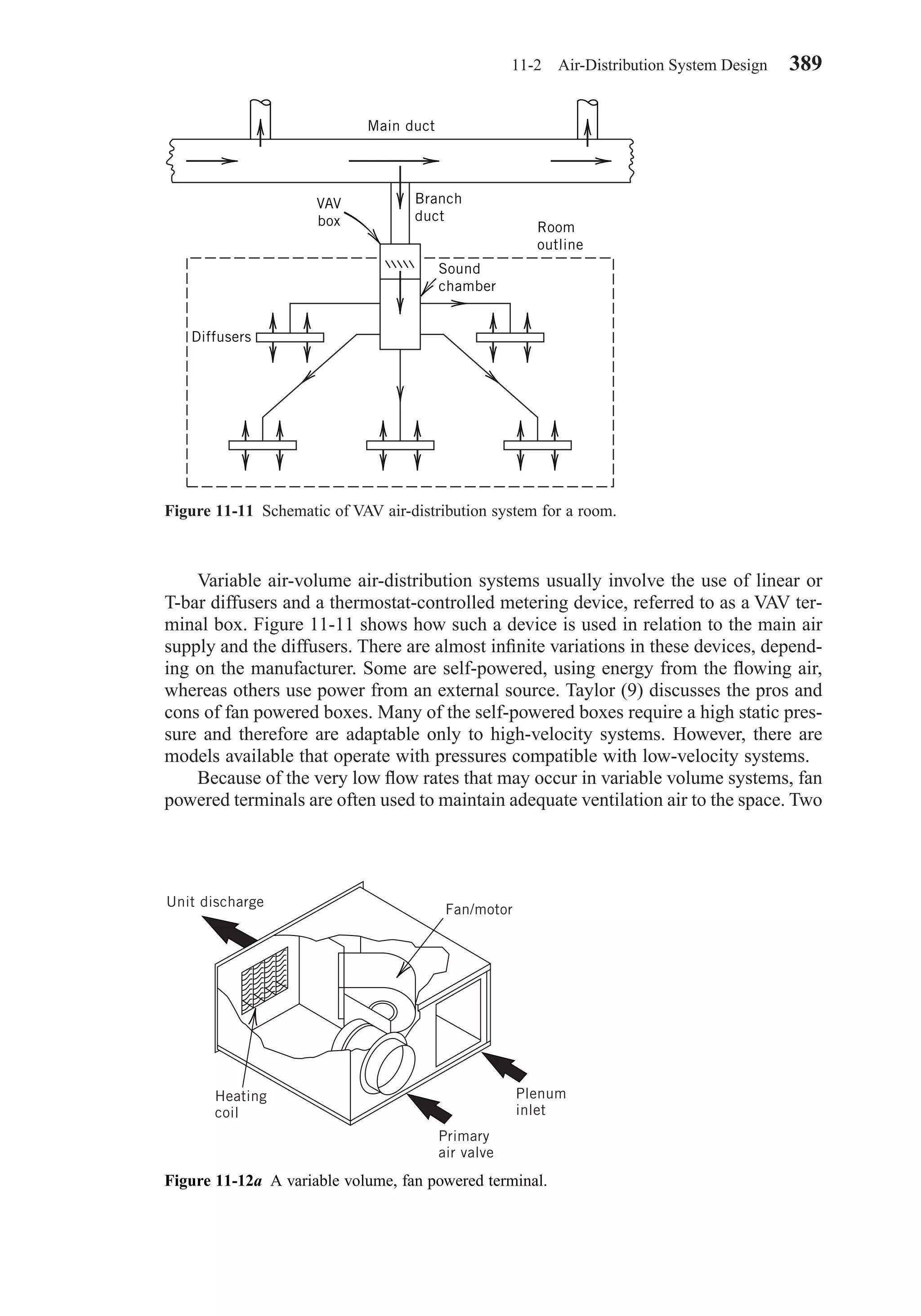
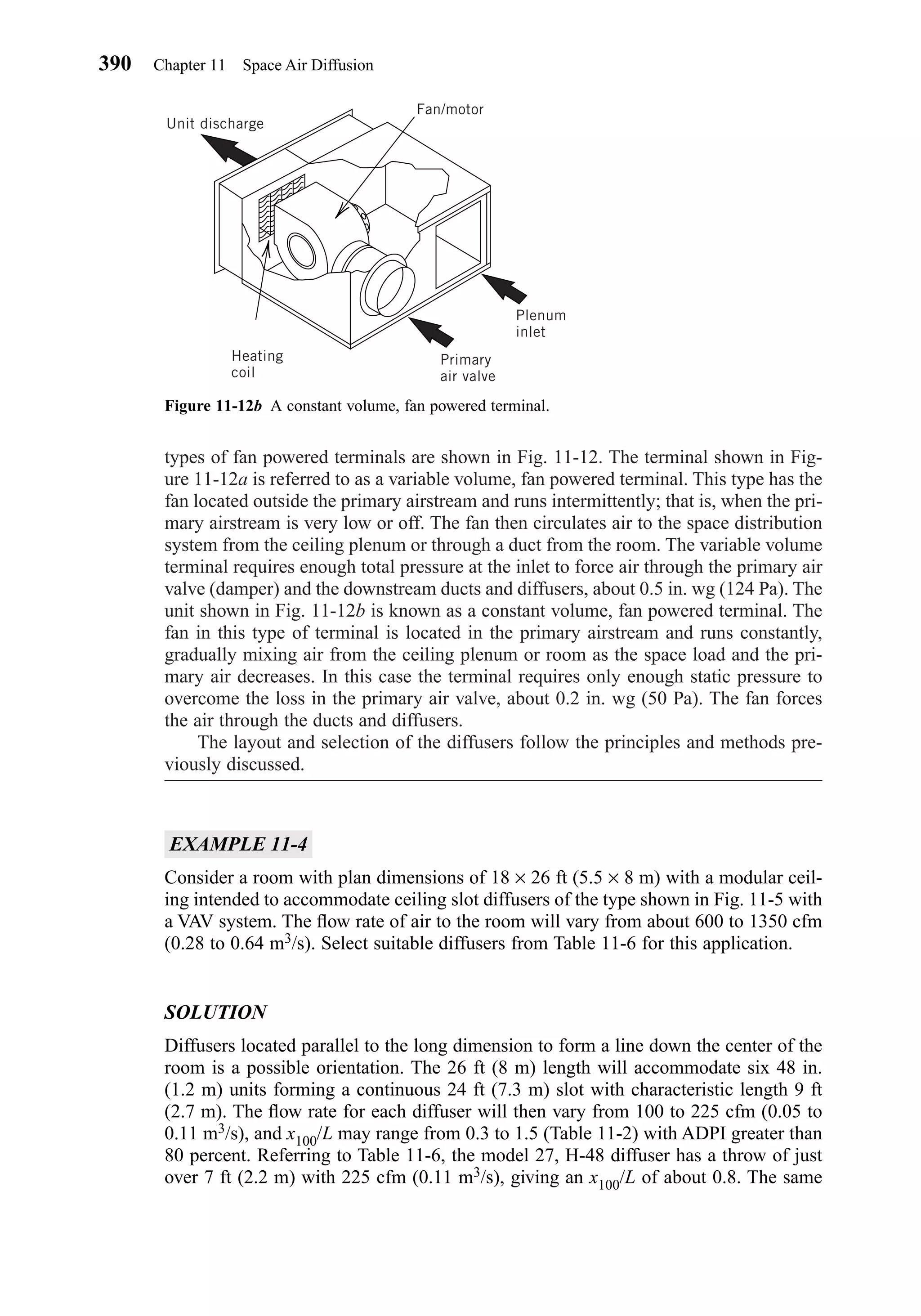
![diffuser with 104 cfm (0.05 m3/s) has x100/L of about 0.44. These values are well
within the acceptable range, and the minimum flow rate could be even less, say 75 cfm
(0.035 m3/s) per diffuser, with satisfactory performance. The maximum total pressure
required is
P0 = 0.18(225/215)2 = 0.2 in. wg = 50 Pa
and the NC is about 32.
REFERENCES
1. ASHRAE Handbook, Fundamentals Volume, American Society of Heating, Refrigerating and Air-Con-
ditioning Engineers, Inc., Atlanta, GA, 2001.
2. Alfred Koestel, “Computing Temperature and Velocities in Vertical Jets of Hot or Cold Air,” ASHVE
Transactions, Vol. 60, 1954.
3. W. E. Blazier, Jr., “RC Mark II: A Refined Procedure for Rating Noise from HVAC Heating, Venti-
lating and Air-Conditioning Systems in Buildings,” Noise Control Eng. J. Vol. 45, No. 6, Novem-
ber/December, 1997.
4. Lawrence J. Gelin, “Active Noise Control: A Tutorial for HVAC Design,” ASHRAE Journal, August
1997.
5. Fred Bauman and Tom Webster, “Outlook for Underfloor Air Distribution,” ASHRAE Journal, June
2001.
6. Alexander M. Zhivov, et al., “A Design Procedure for Displacement Ventilation,” Heating, Piping and
Air Conditioning, Part I, November 2000.
7. ASHRAE, Designers Guide to Ceiling-Based Air Diffusion, Product Code No. 90425, American Soci-
ety of Heating, Refrigerating and Air-Conditioning Engineers, Inc., Atlanta, GA.
8. J. Rydberg and P. Norback, “ASHVE Research Report No. 1362 – Air Distribution and Draft,” ASHVE
Transactions, Vol. 65, 1949.
9. Steven C. Taylor, “Series Fan-Powered Boxes,” ASHRAE Journal, July 1996.
PROBLEMS
11-1. A free isothermal jet is discharged horizontally from a circular opening. There is no nearby sur-
face. The initial velocity and volume flow rate are 850 ft/min (4.3 m/s) and 300 cfm (142 L/s),
respectively. Estimate (a) the throw for terminal velocities of 50, 100, and 150 ft/min (0.25,
0.50, 0.75 m/s) and (b) the total volume flow rate of the jet for each terminal velocity in (a).
11-2. A free jet is discharged horizontally below a ceiling. The initial velocity and volume flow rate
are 1100 ft/min (5.6 m/s) and 300 cfm (165 L/s). The initial jet temperature is 100 F (38 C),
whereas the room is to be maintained at 72 F (22 C). Compute the throw and the difference in
temperature between the center line of the jet and the room at terminal velocities of 50, 100,
and 150 ft/min (0.25, 0.50, and 0.75 m/s, respectively).
11-3. To ventilate a space, it is desired to discharge free isothermal jets vertically downward from a
ceiling 24 ft (7.3 m) above the floor. The terminal velocity of the jets should be no more than
50 ft/min (0.25 m/s), 6 ft (1.83 m) above the floor. Determine a reasonable diameter and initial
volume flow rate for each jet [D0 < 12 in. (30 cm)].
11-4. A free isothermal jet of 125 cfm (60 L/s), 6 in. (15 cm) diameter, is discharged vertically from
the floor toward a ventilation hood 12 ft (3.7 m) above the floor. Approximately what capacity
must the hood exhaust fan have to capture all of the airstream at the entrance to the hood?
11-5. A given space requires a very large quantity of circulated air for cooling purposes. What type
of diffuser system would be best? Why?
11-6. Consider a single-story structure with many windows. What would be the best all-around air-
distribution system for (a) the northern part of the United States and (b) the southern states?
Explain.
Problems 391
Chapter11.qxd 6/15/04 2:37 PM Page 391](https://image.slidesharecdn.com/fayec-160521192803/75/Faye-c-mc_quiston_-_jerald_d-_parker_-_jeffrey_d-409-2048.jpg)
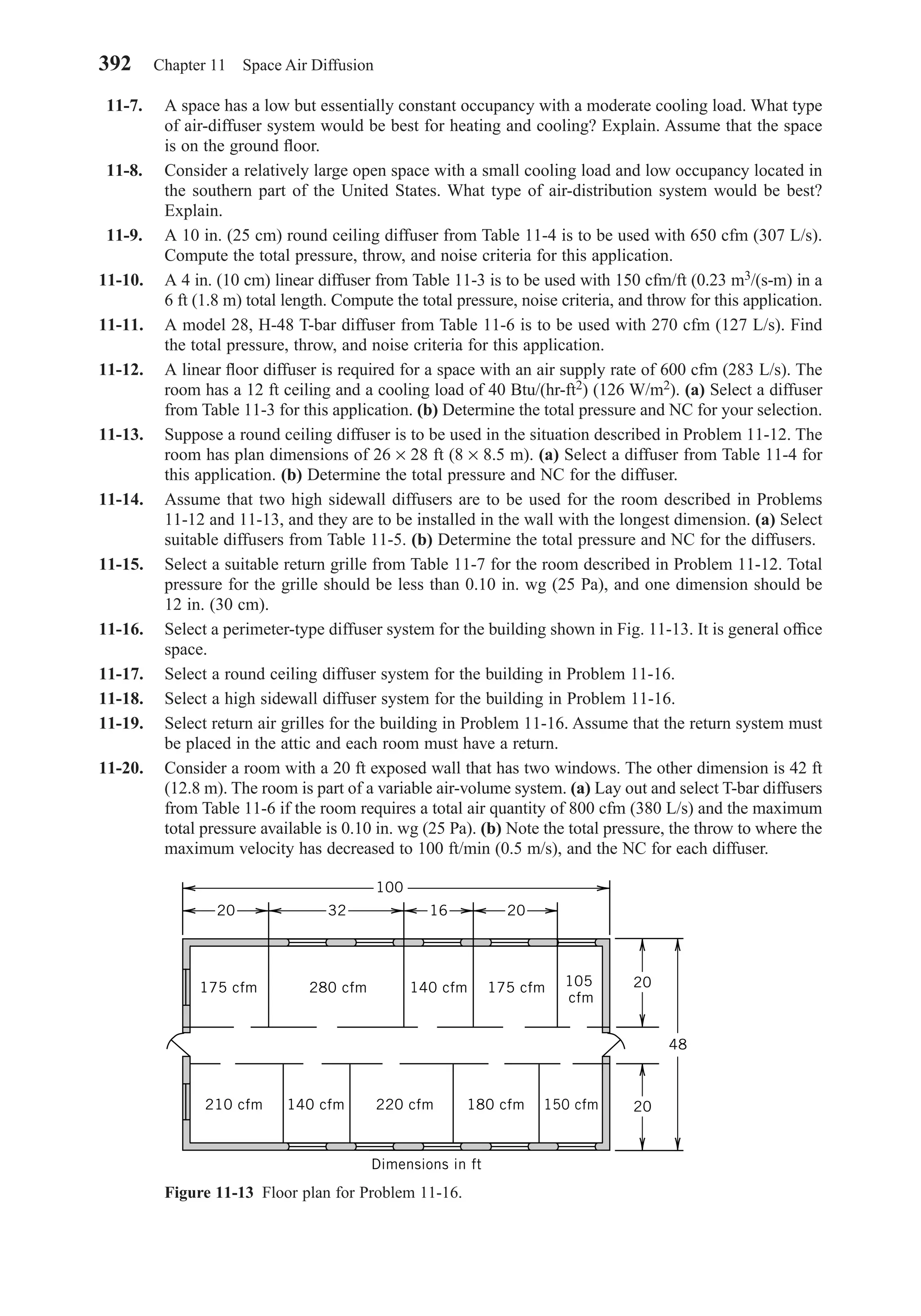

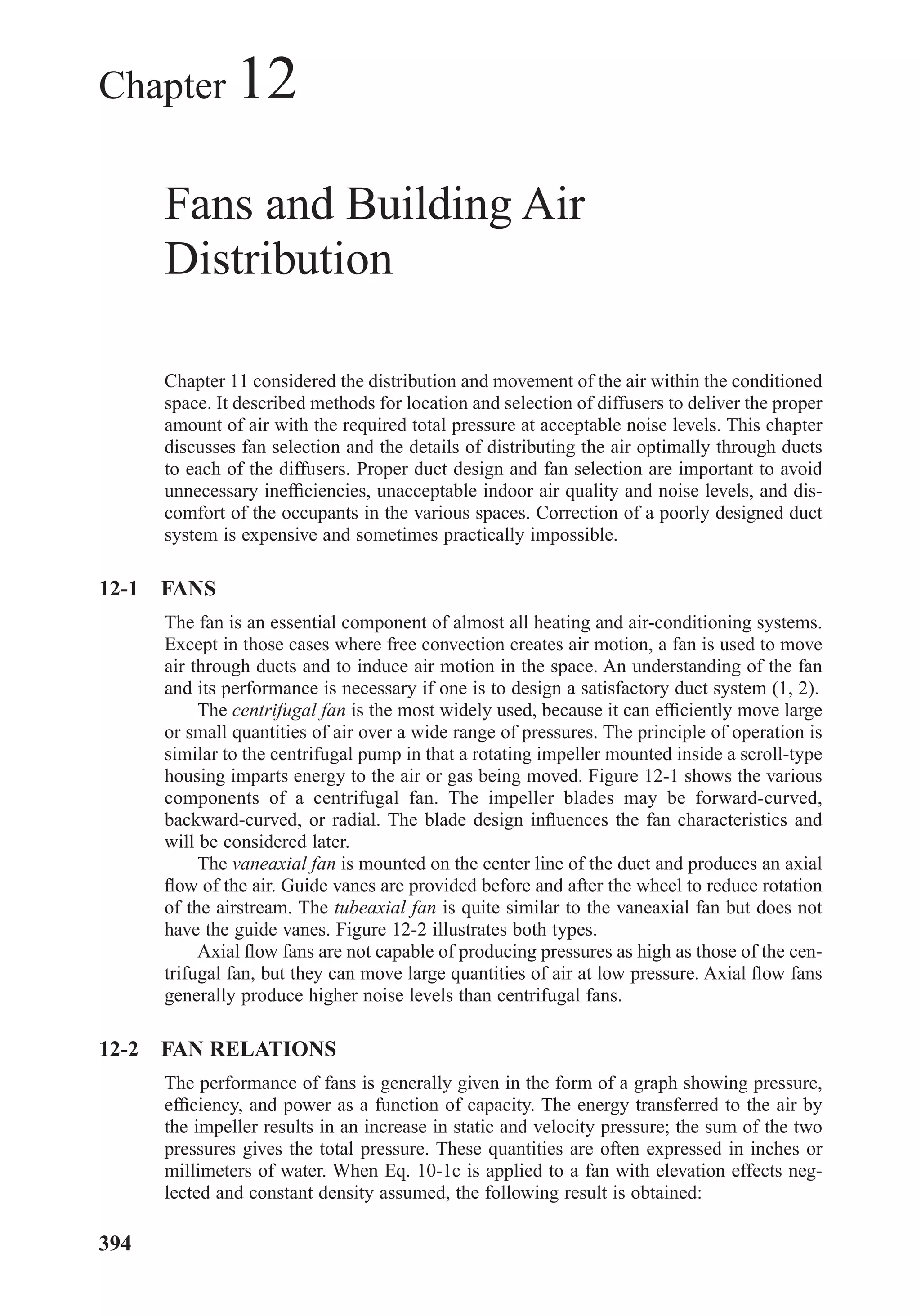
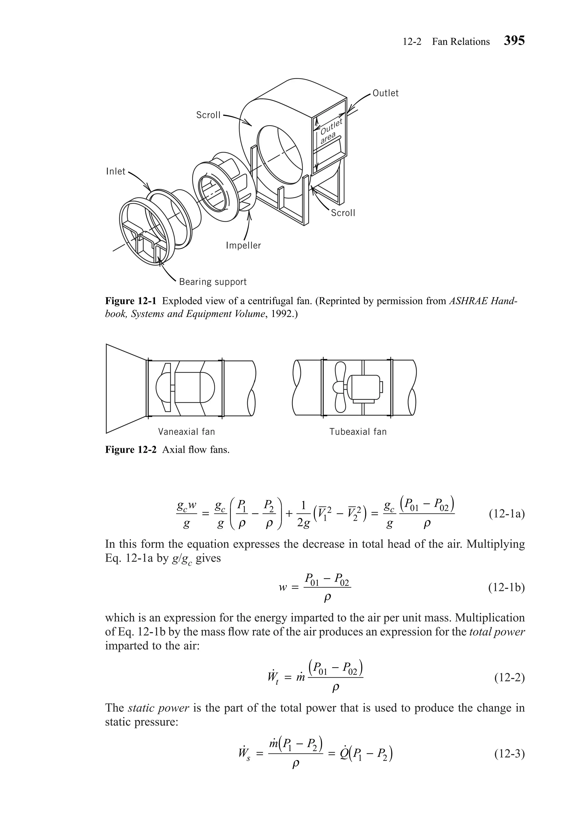
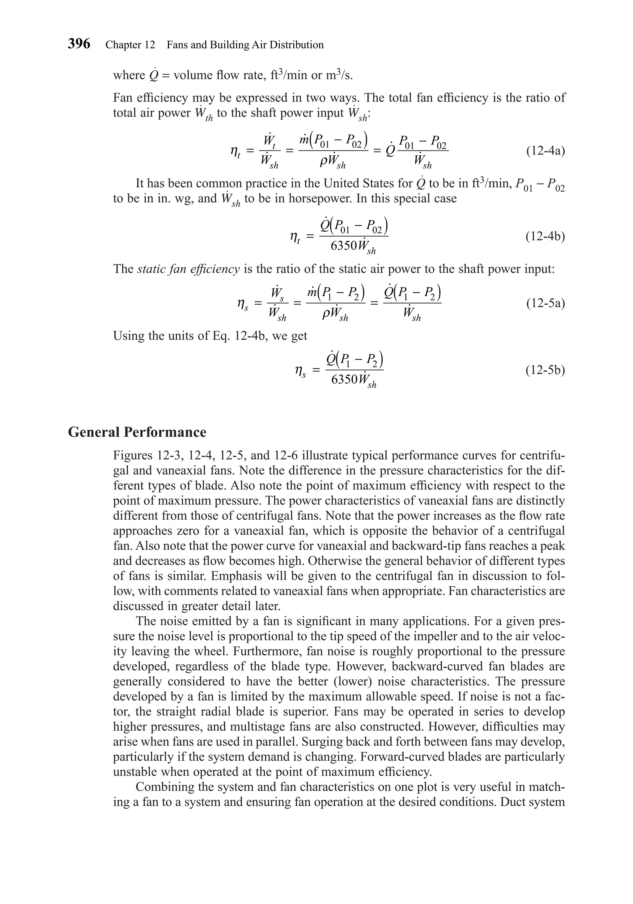
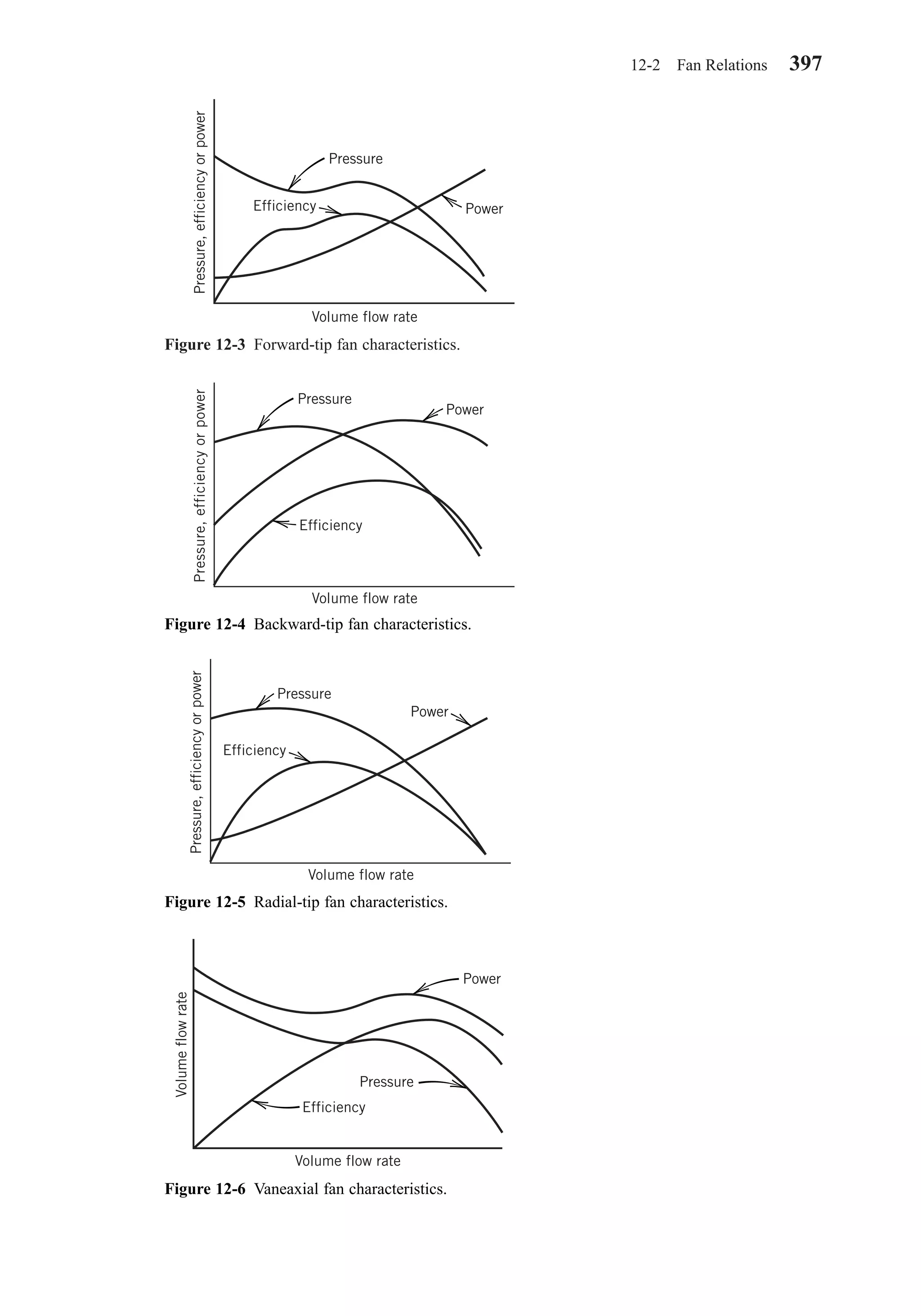
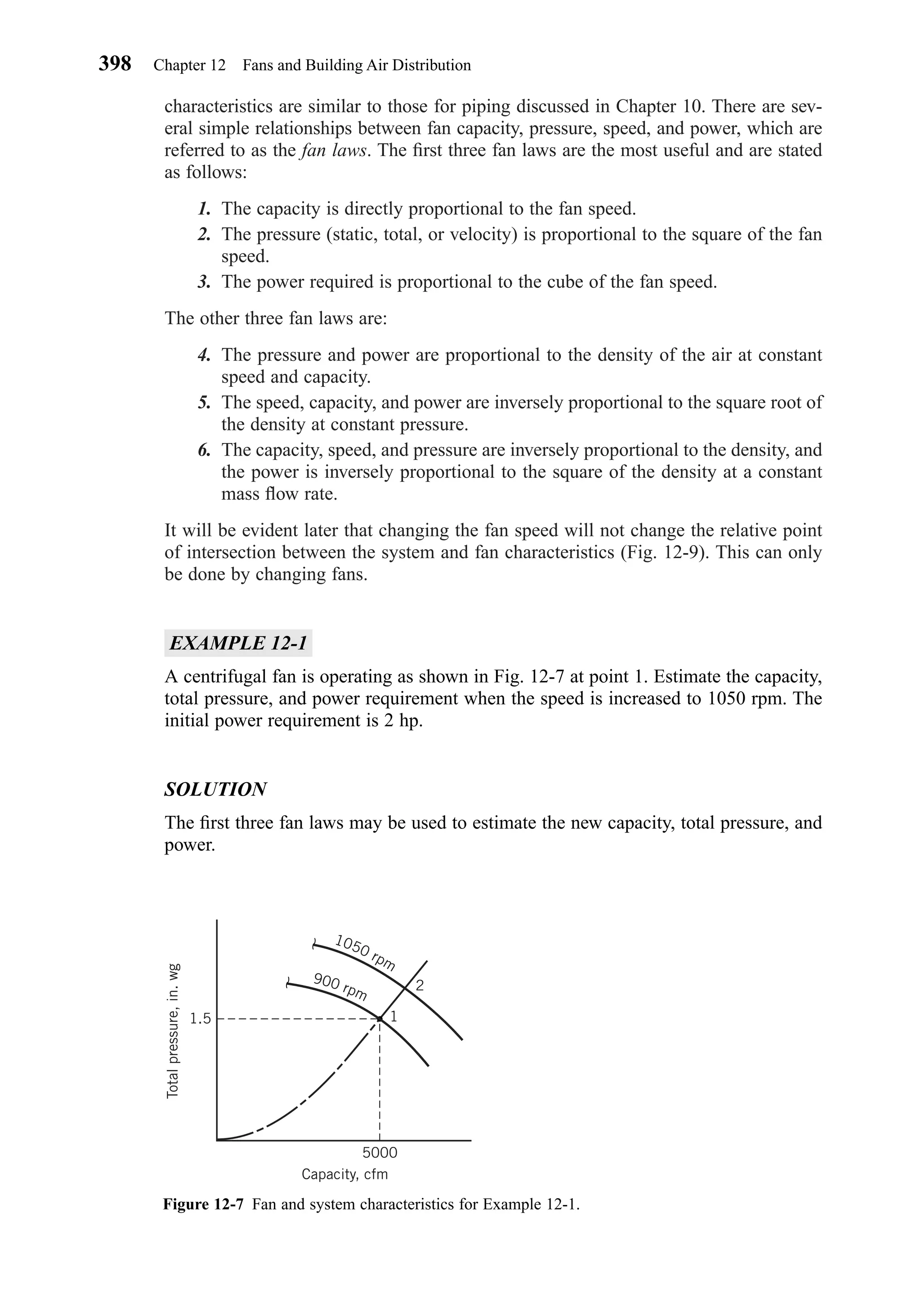
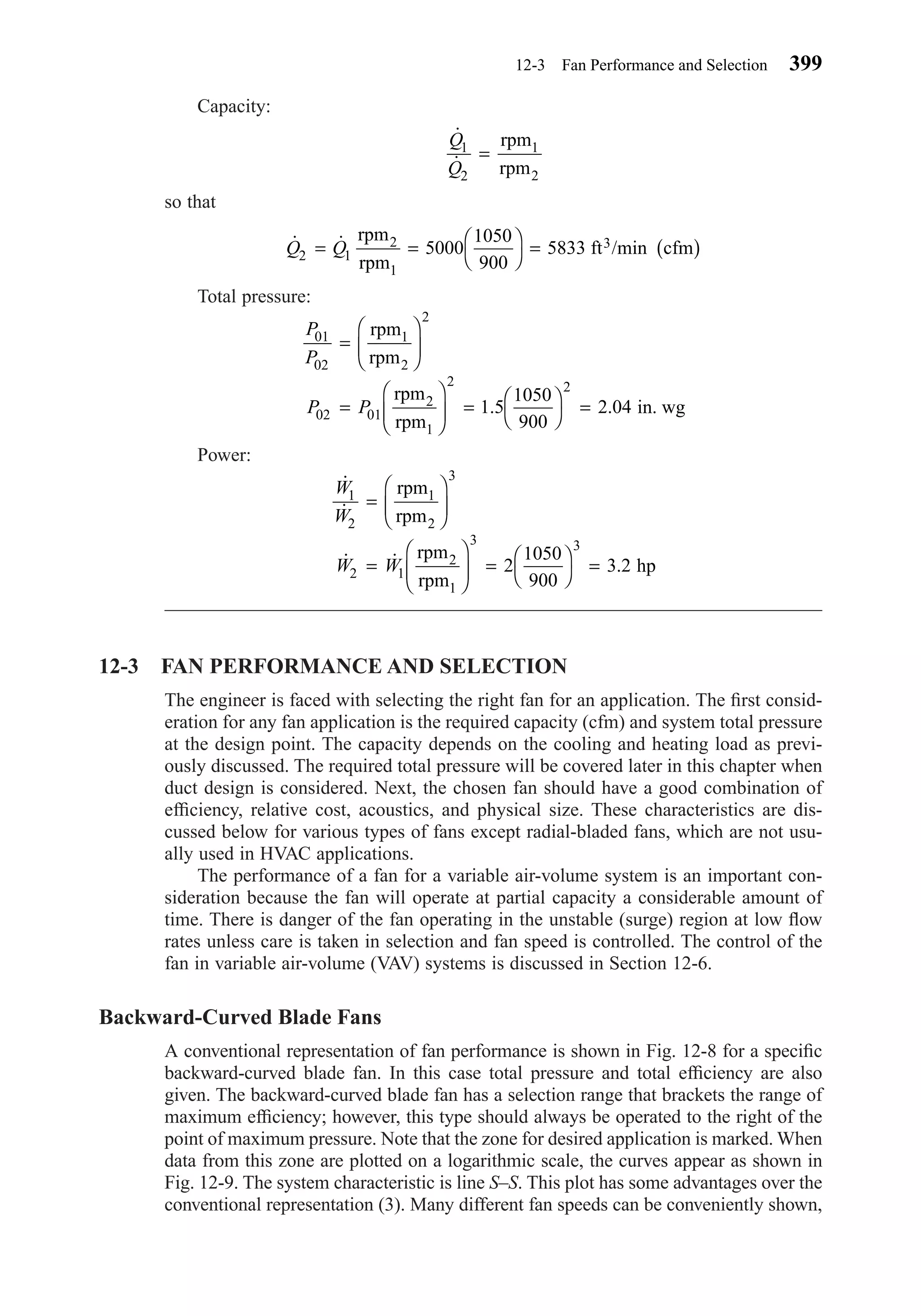
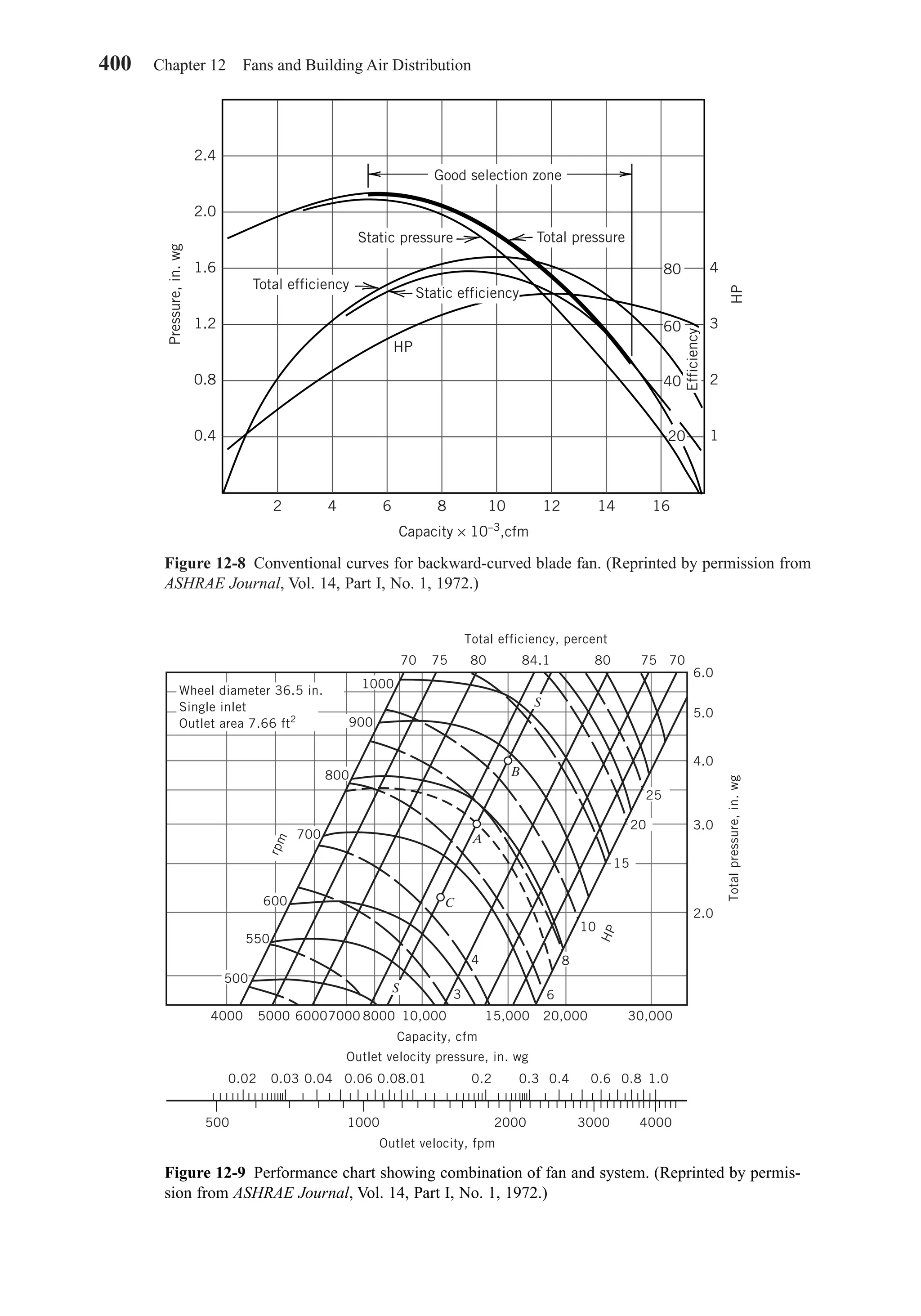
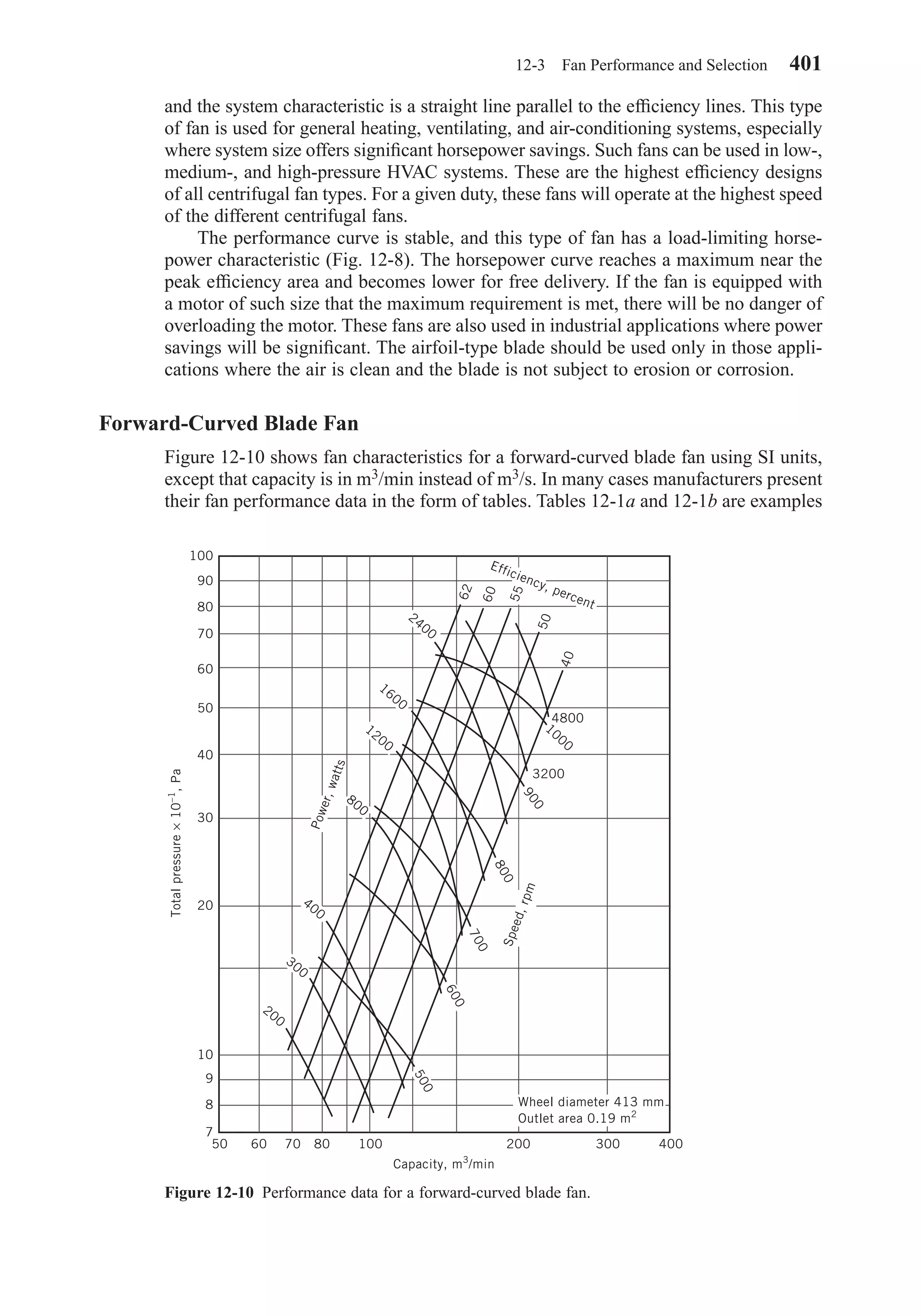
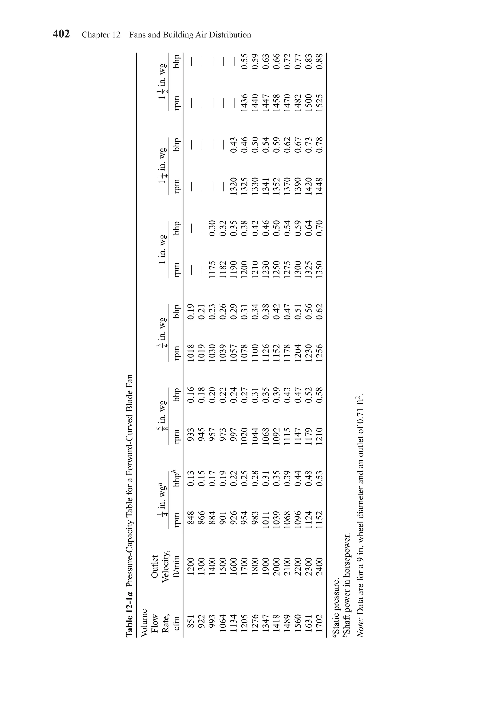
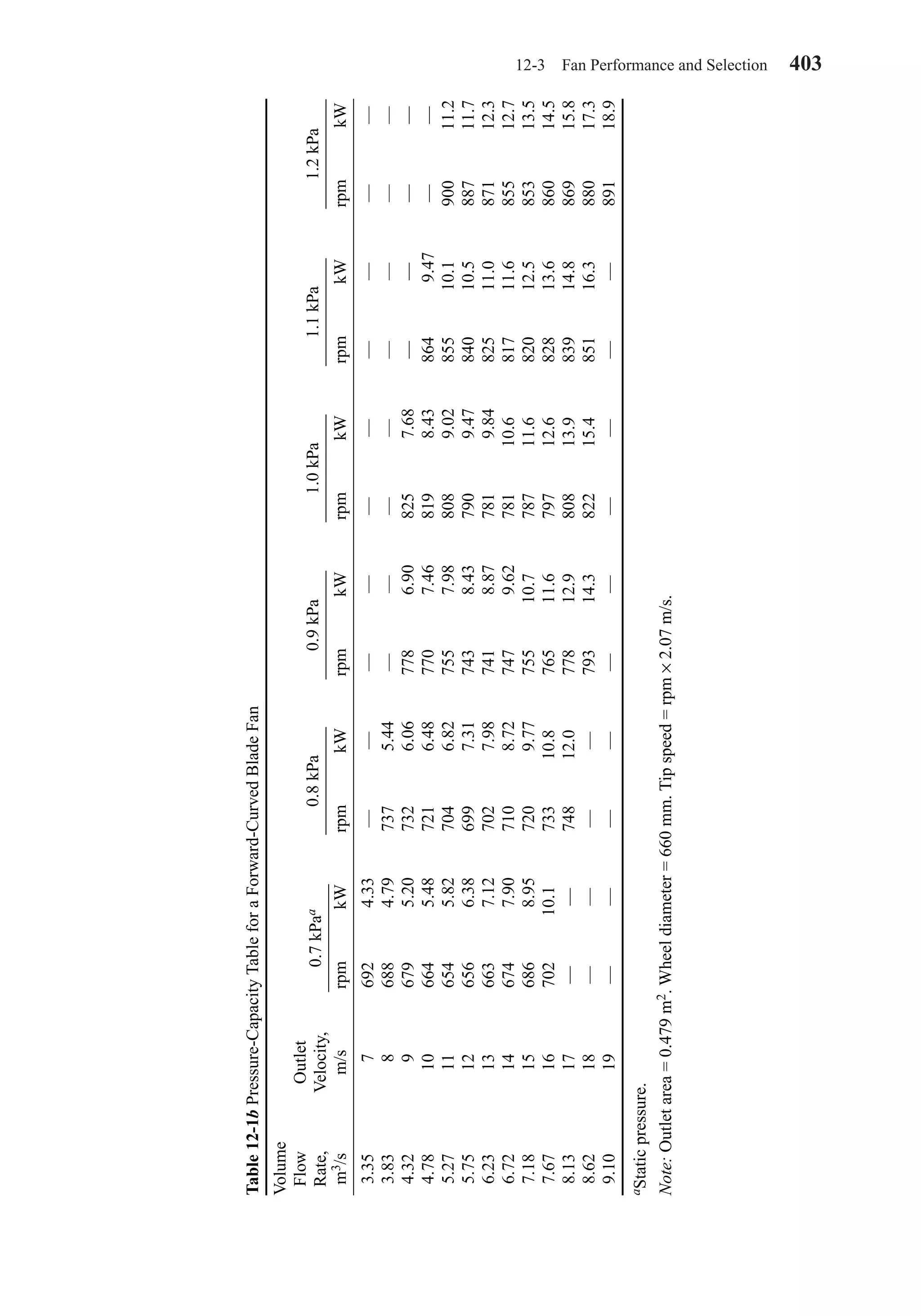
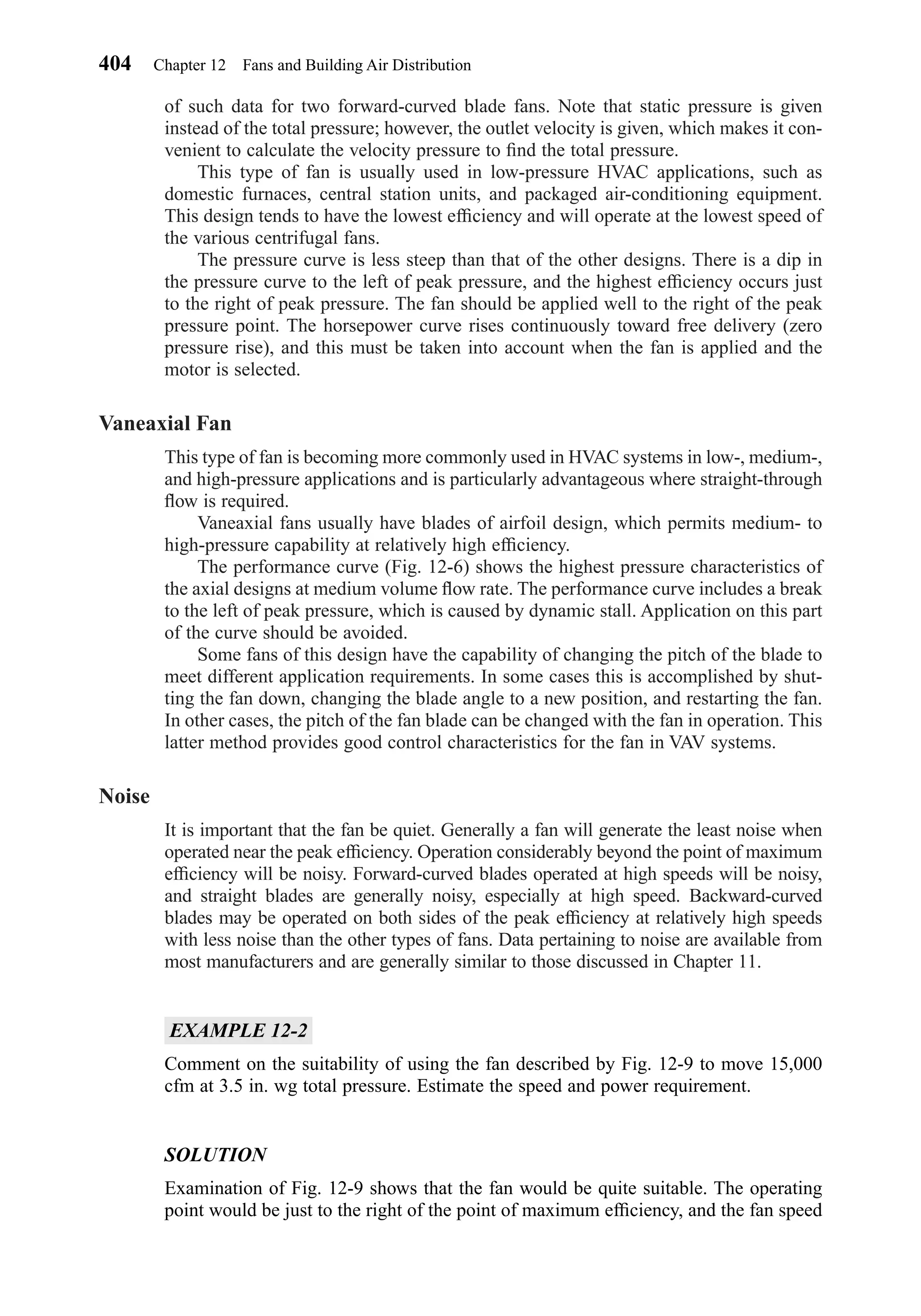
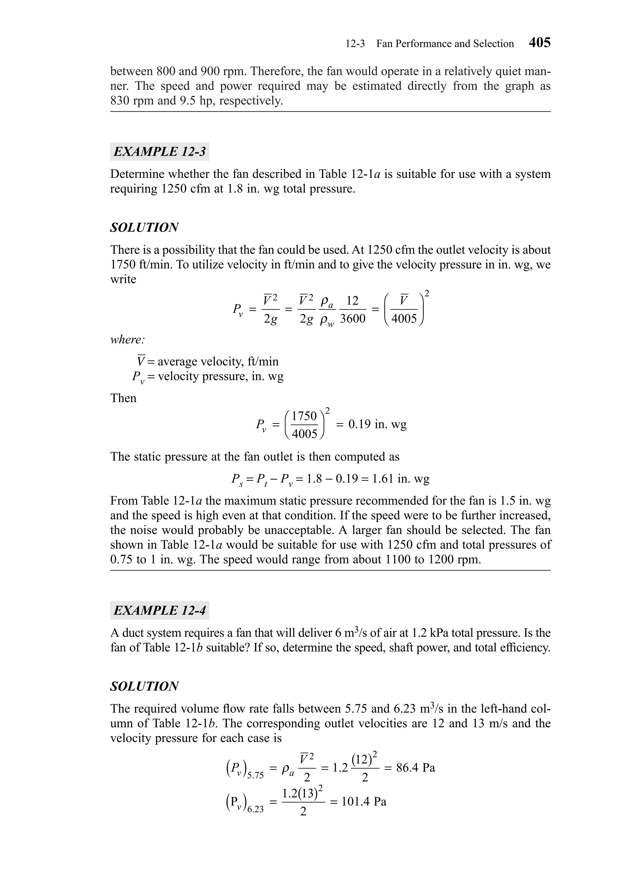
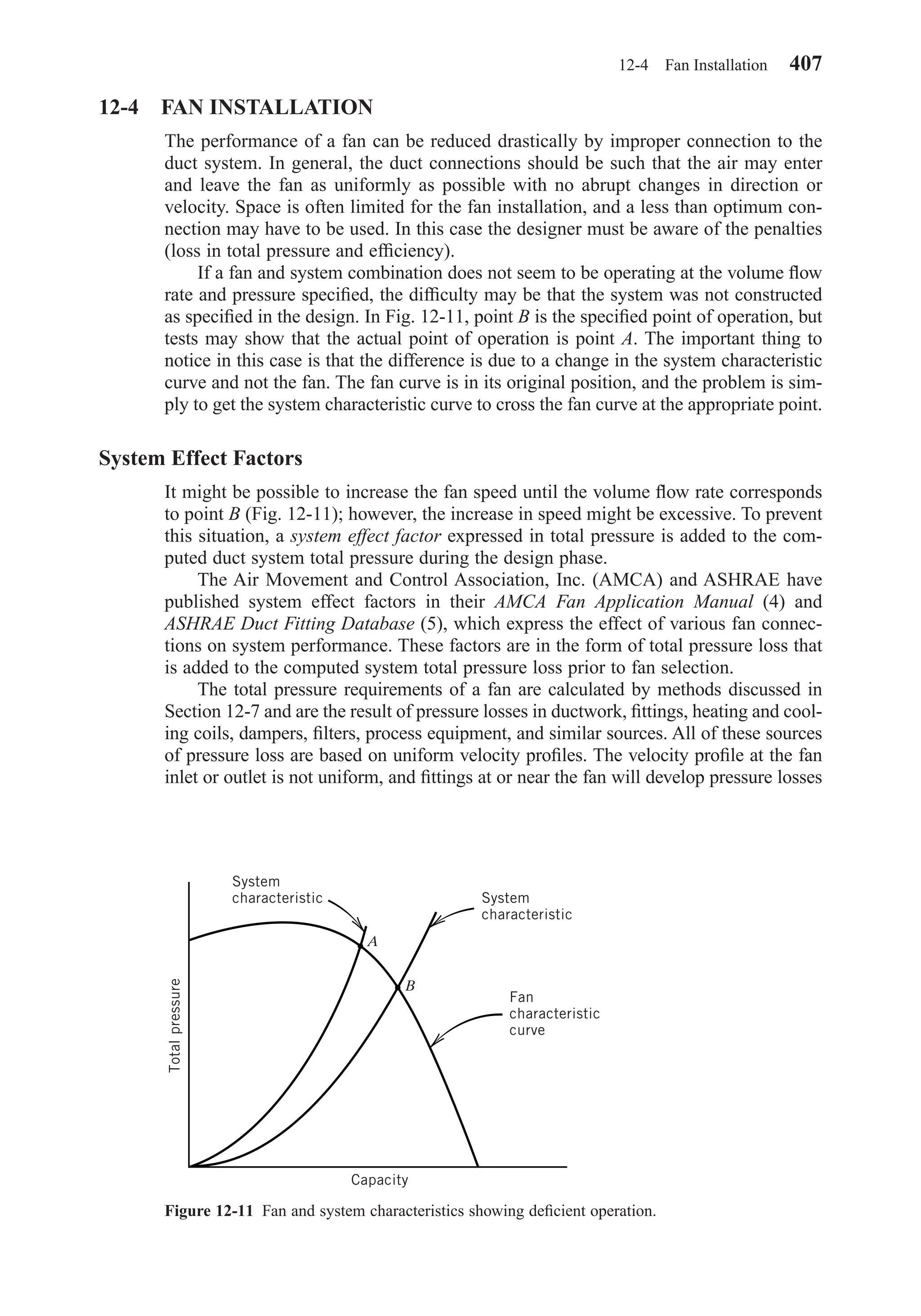
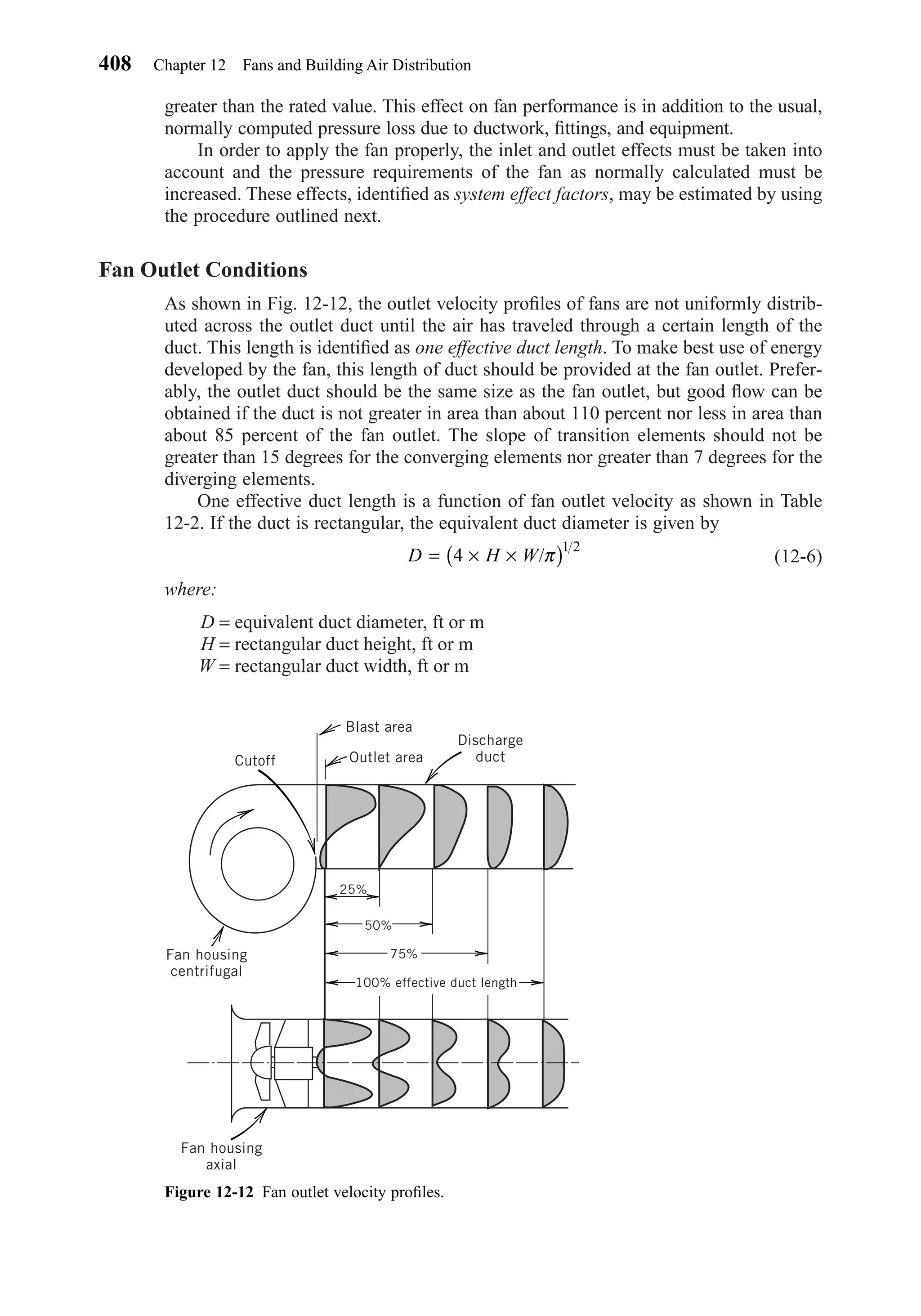
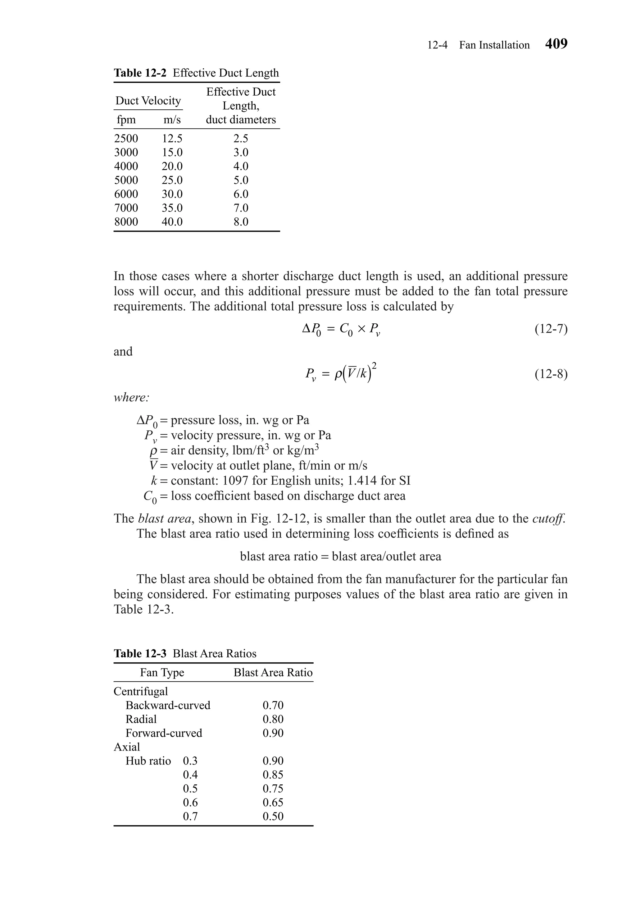
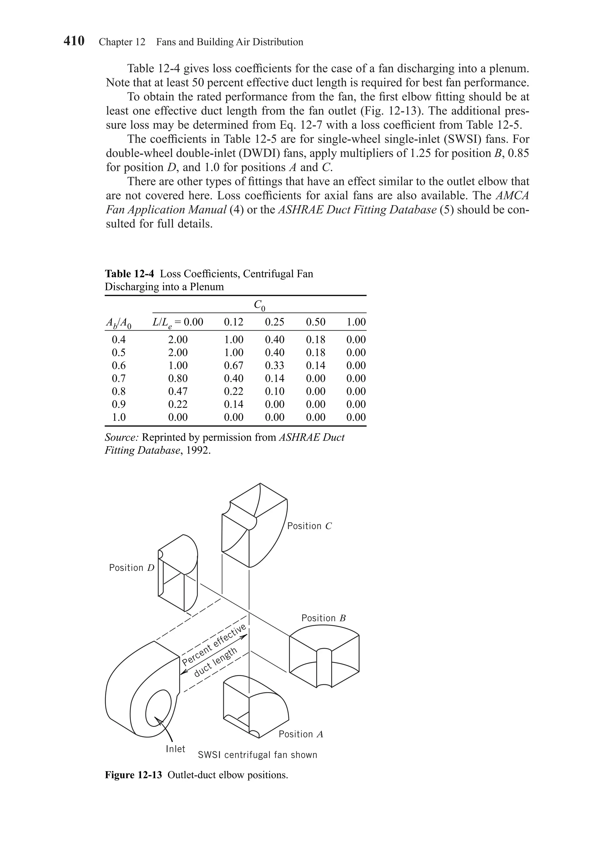
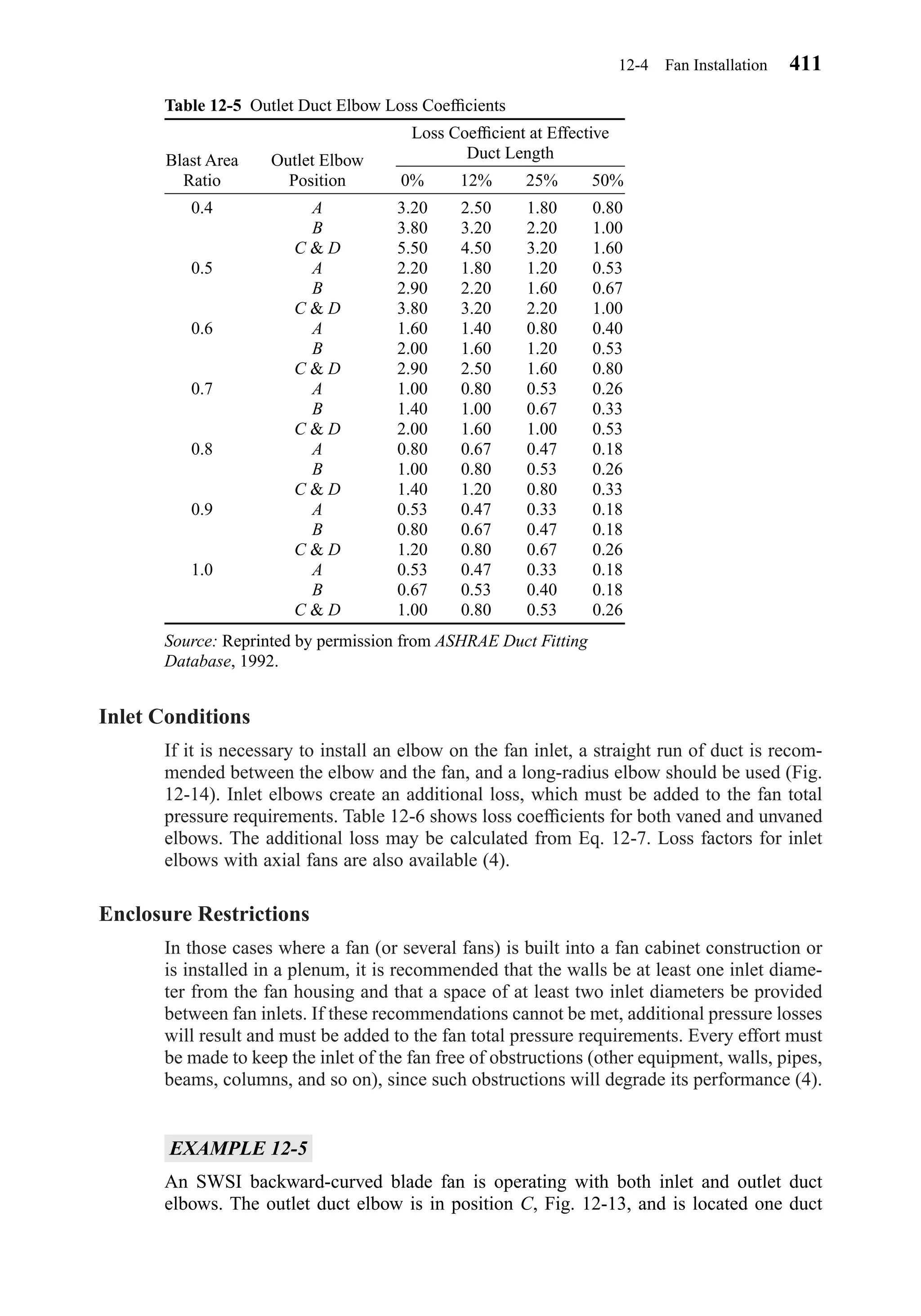
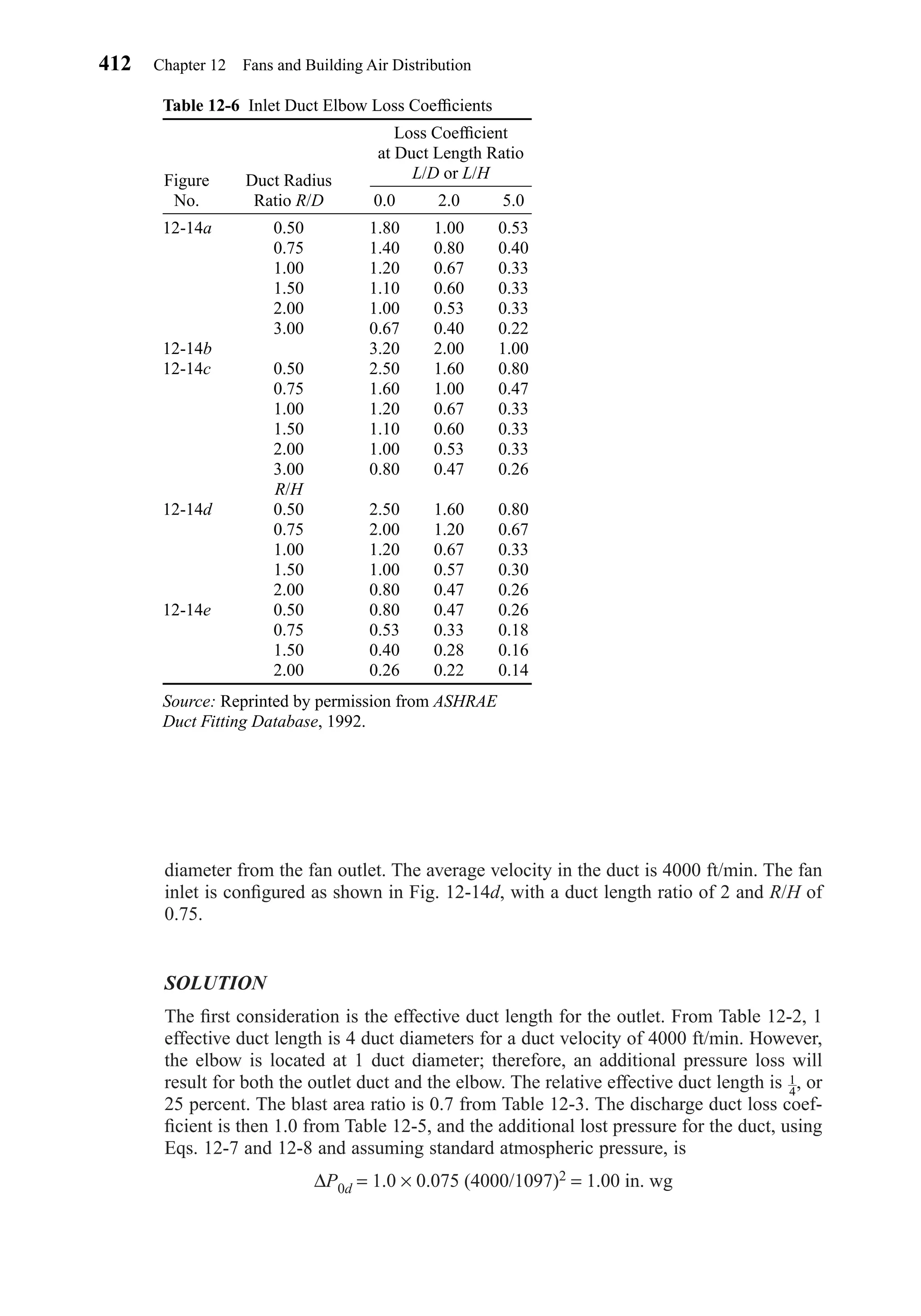
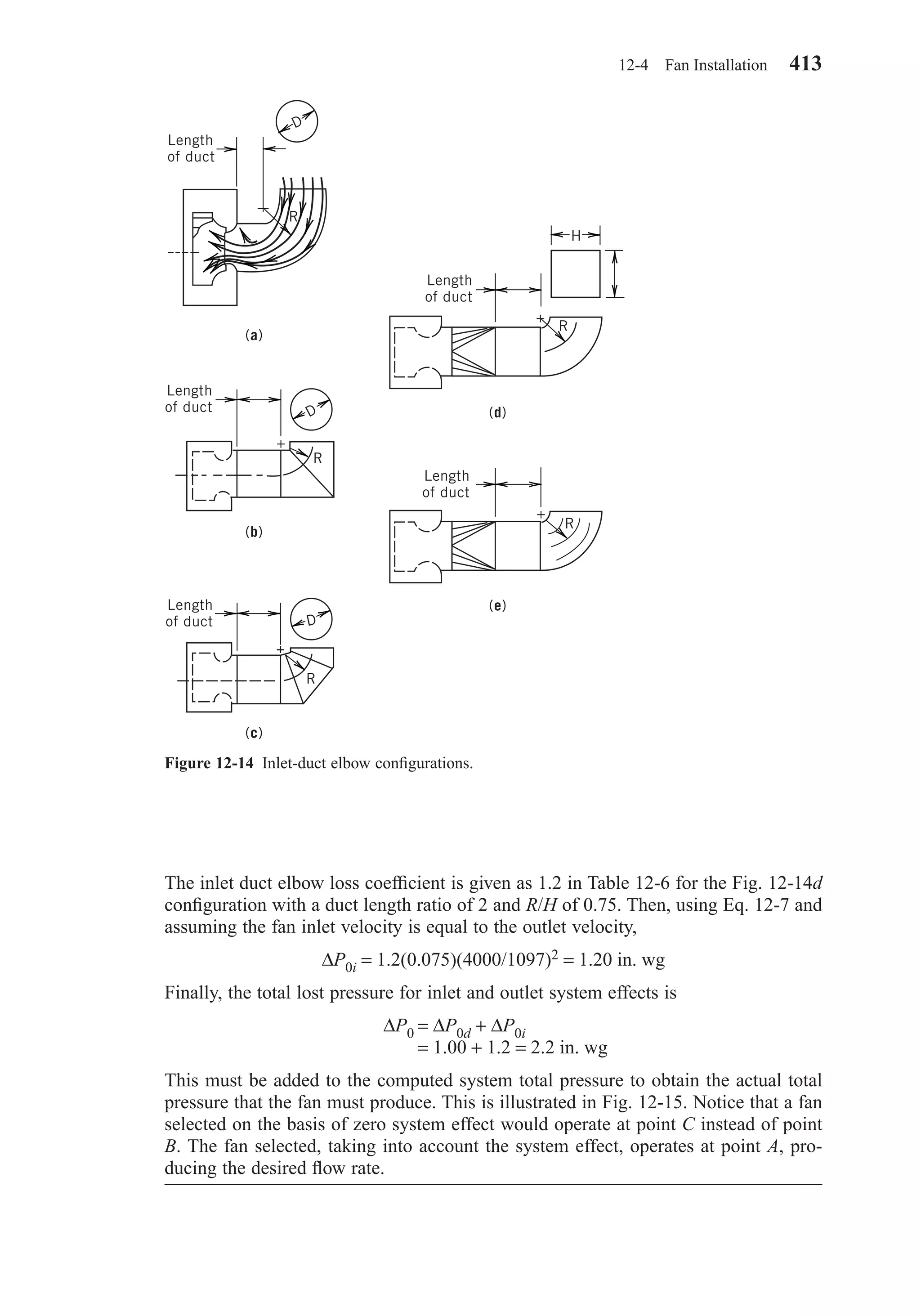
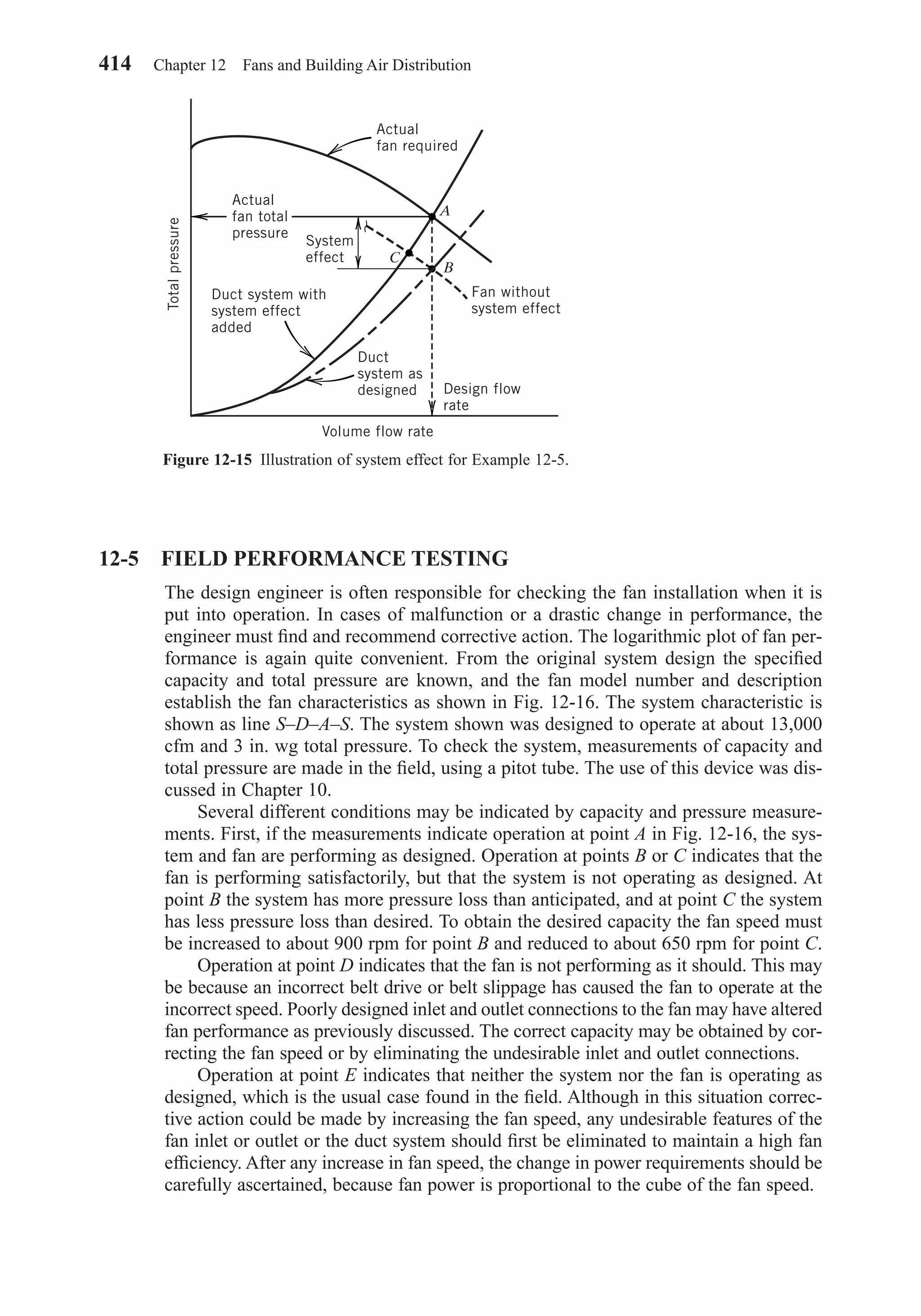
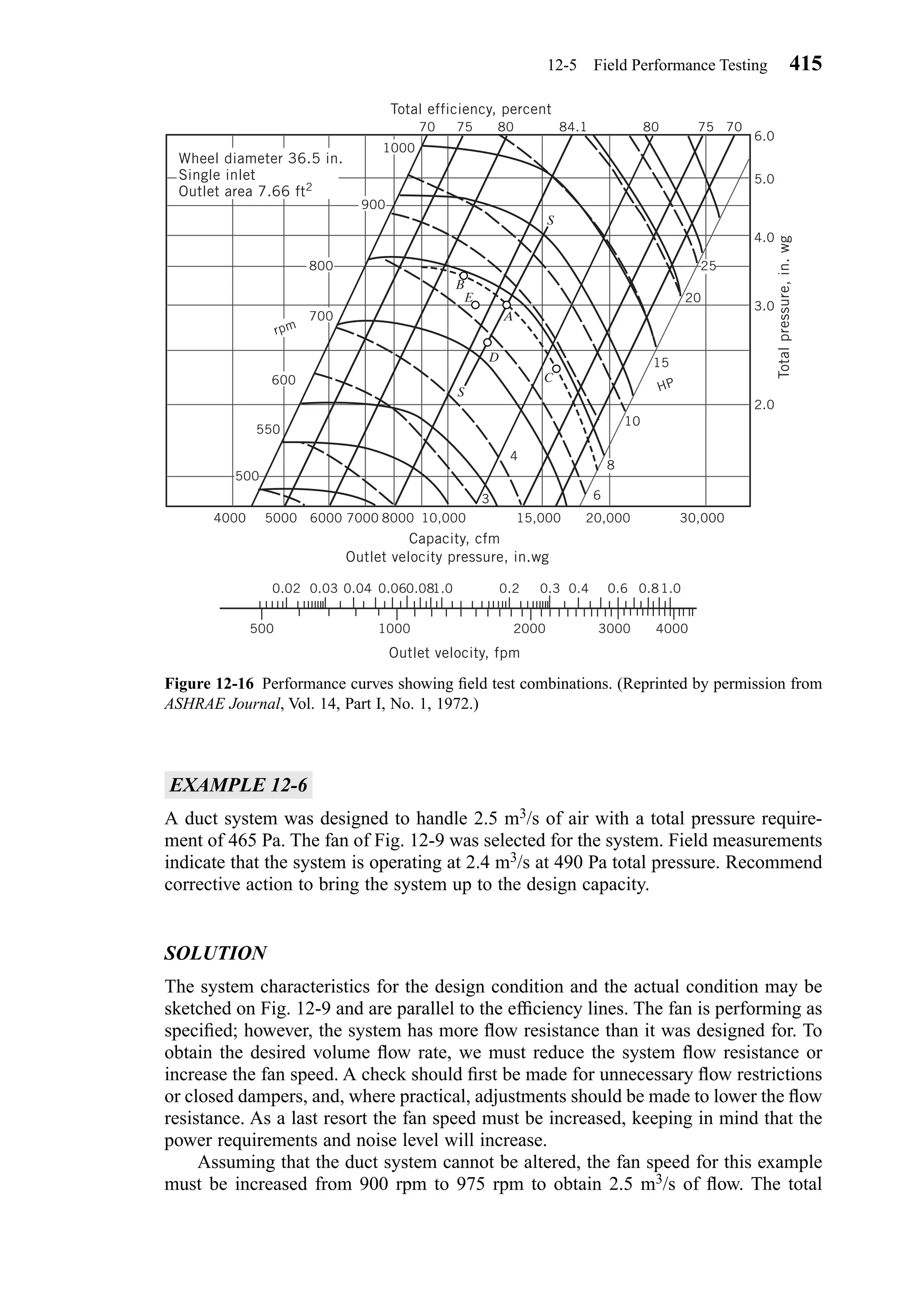
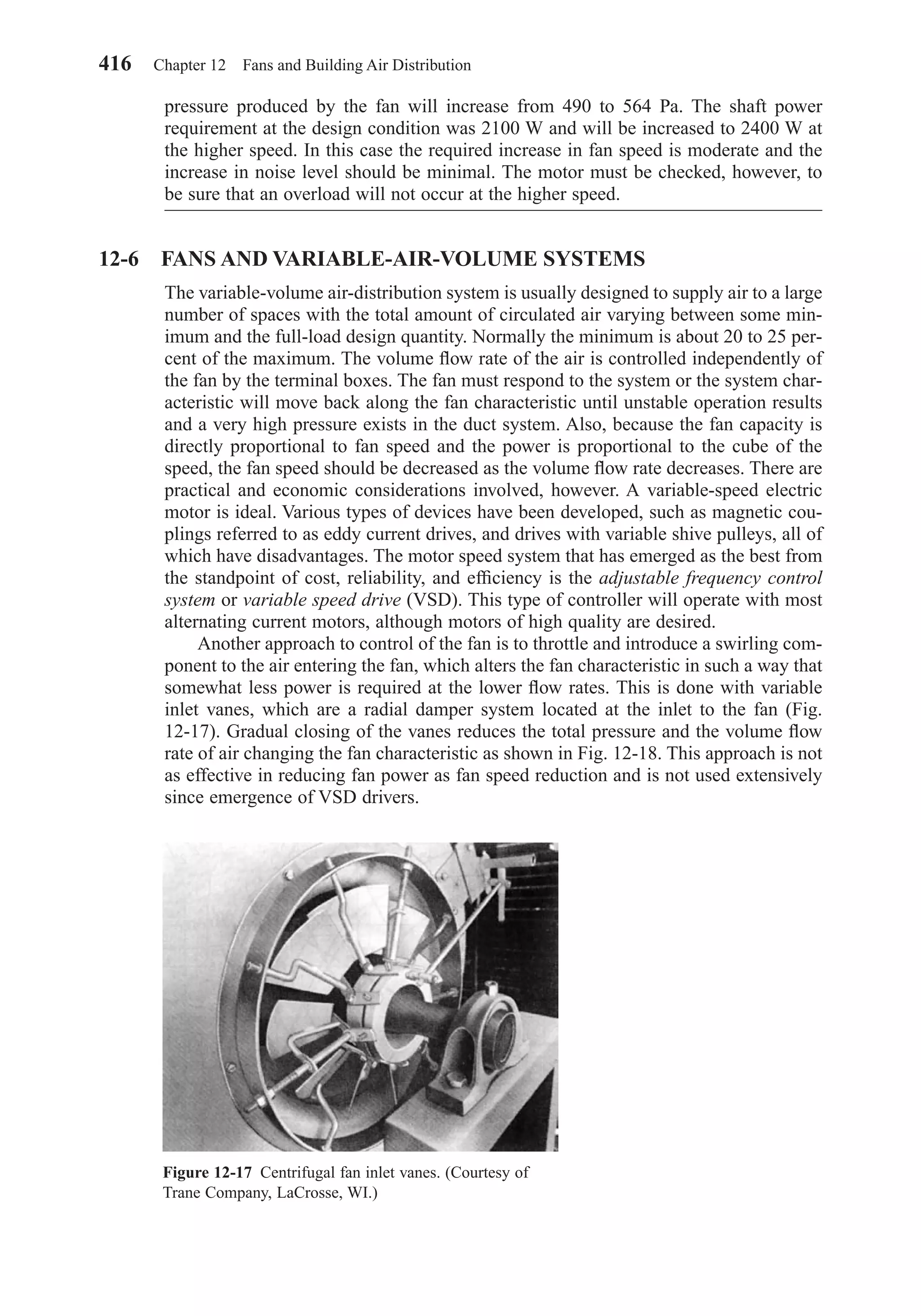
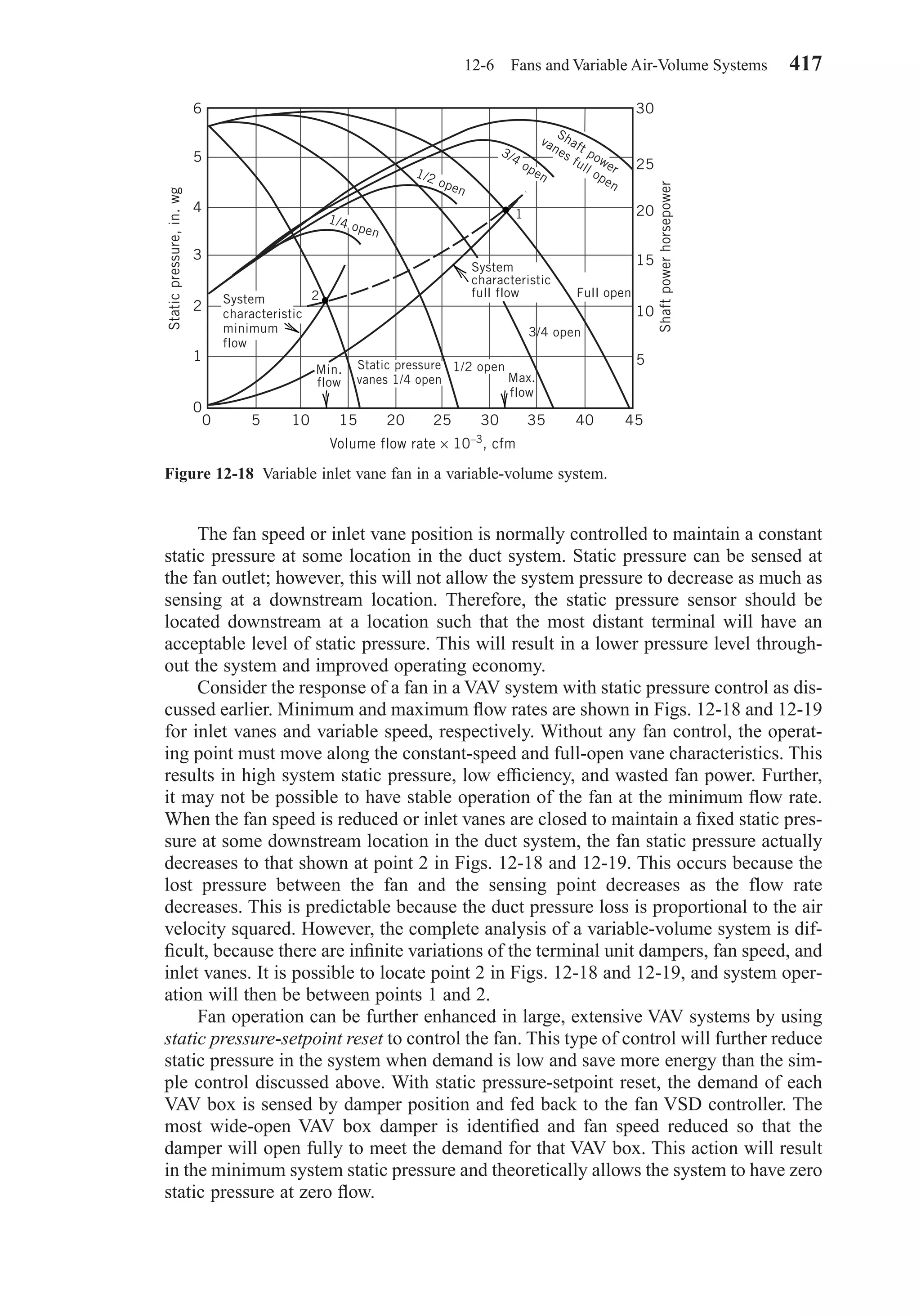
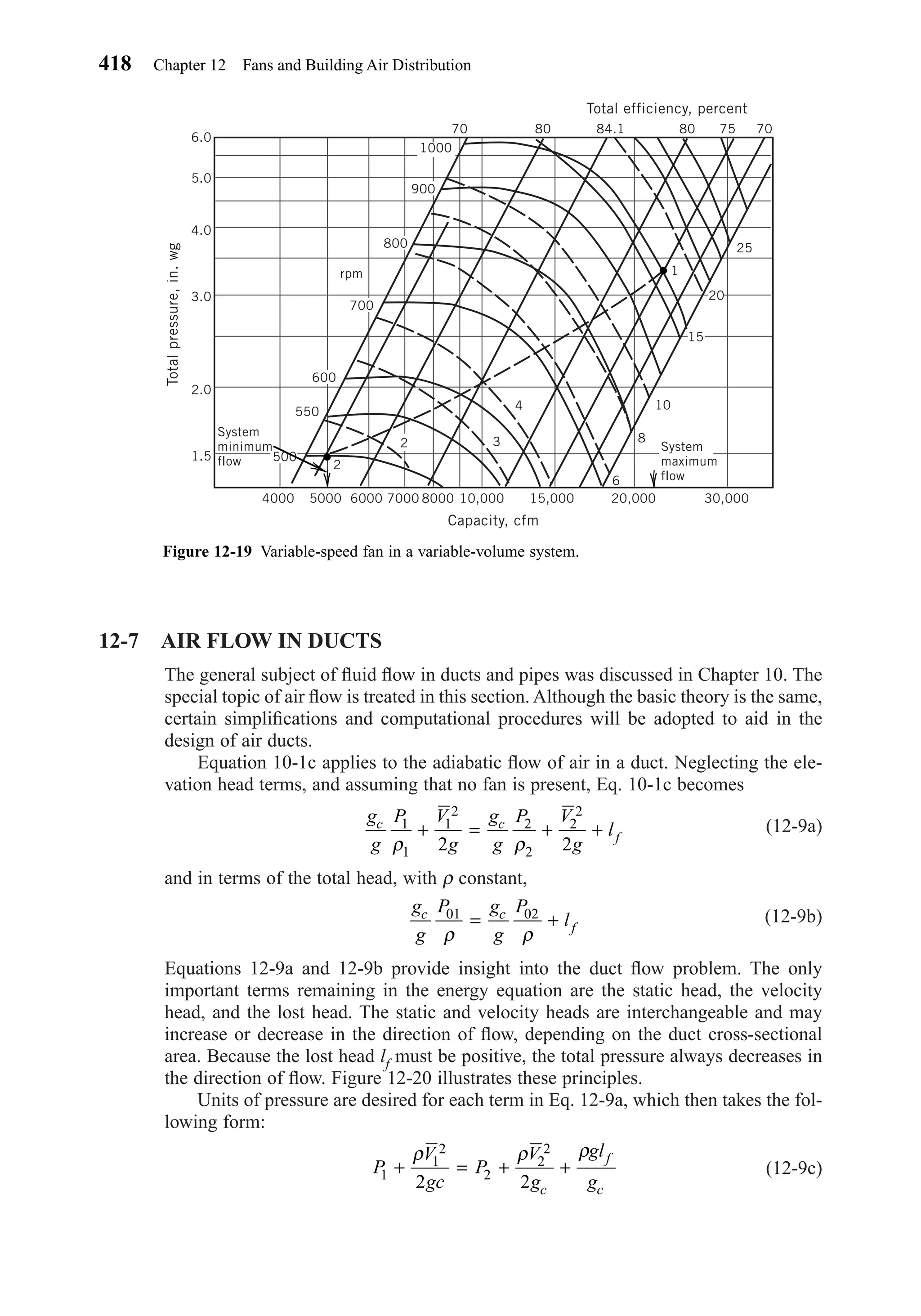
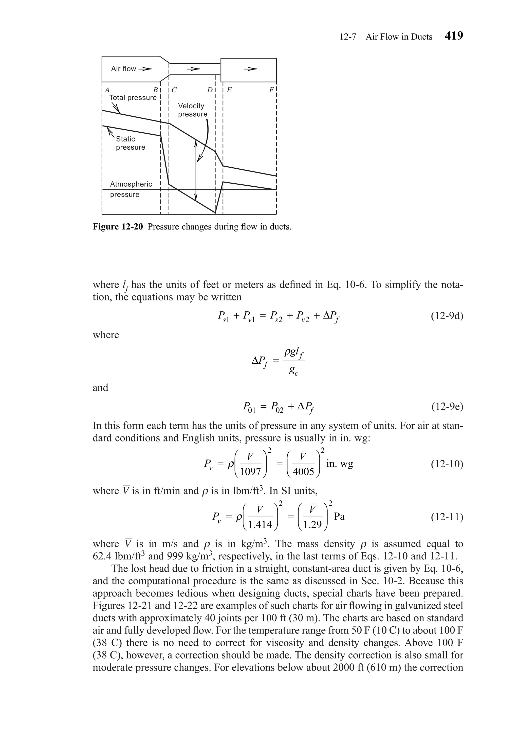
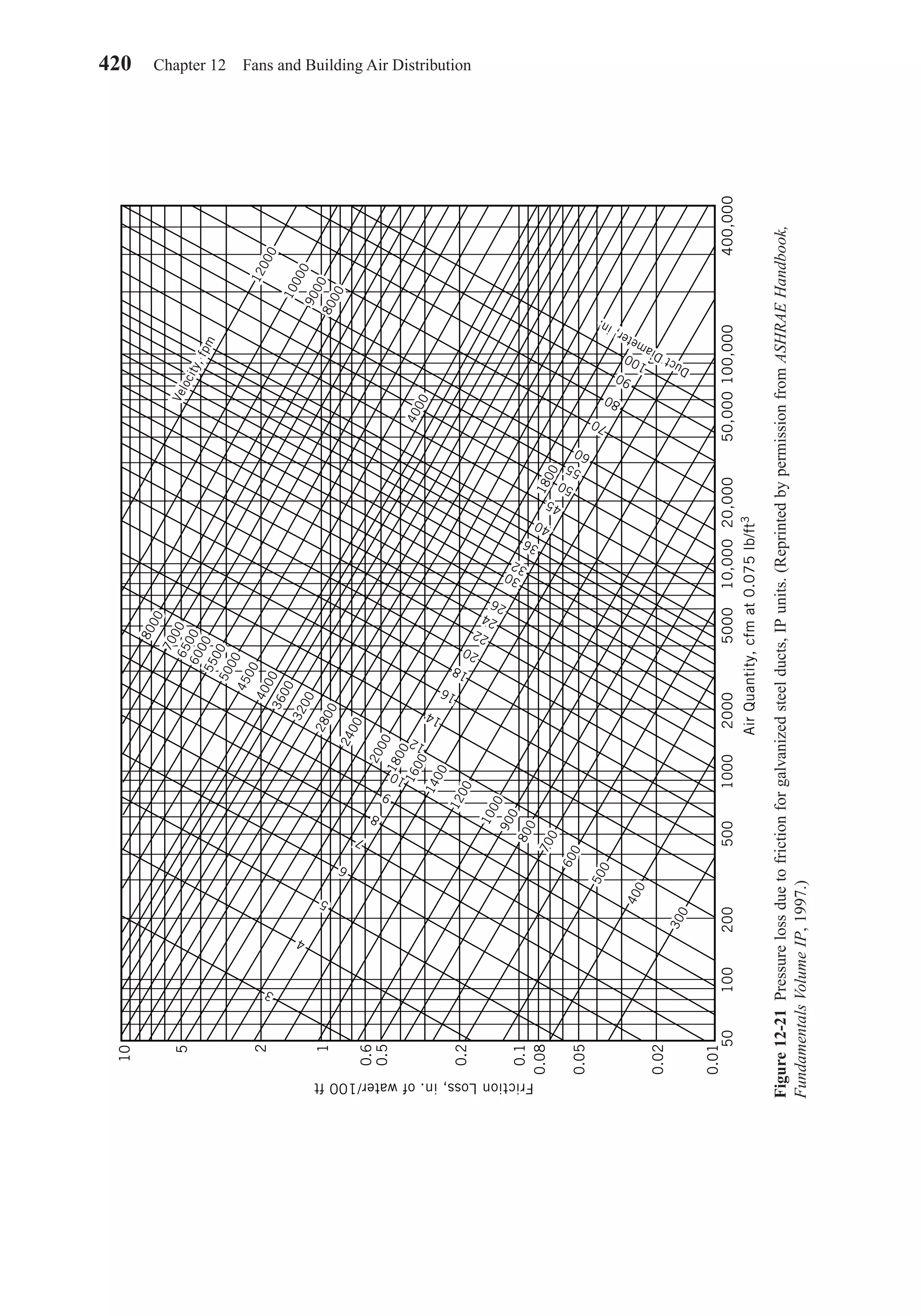
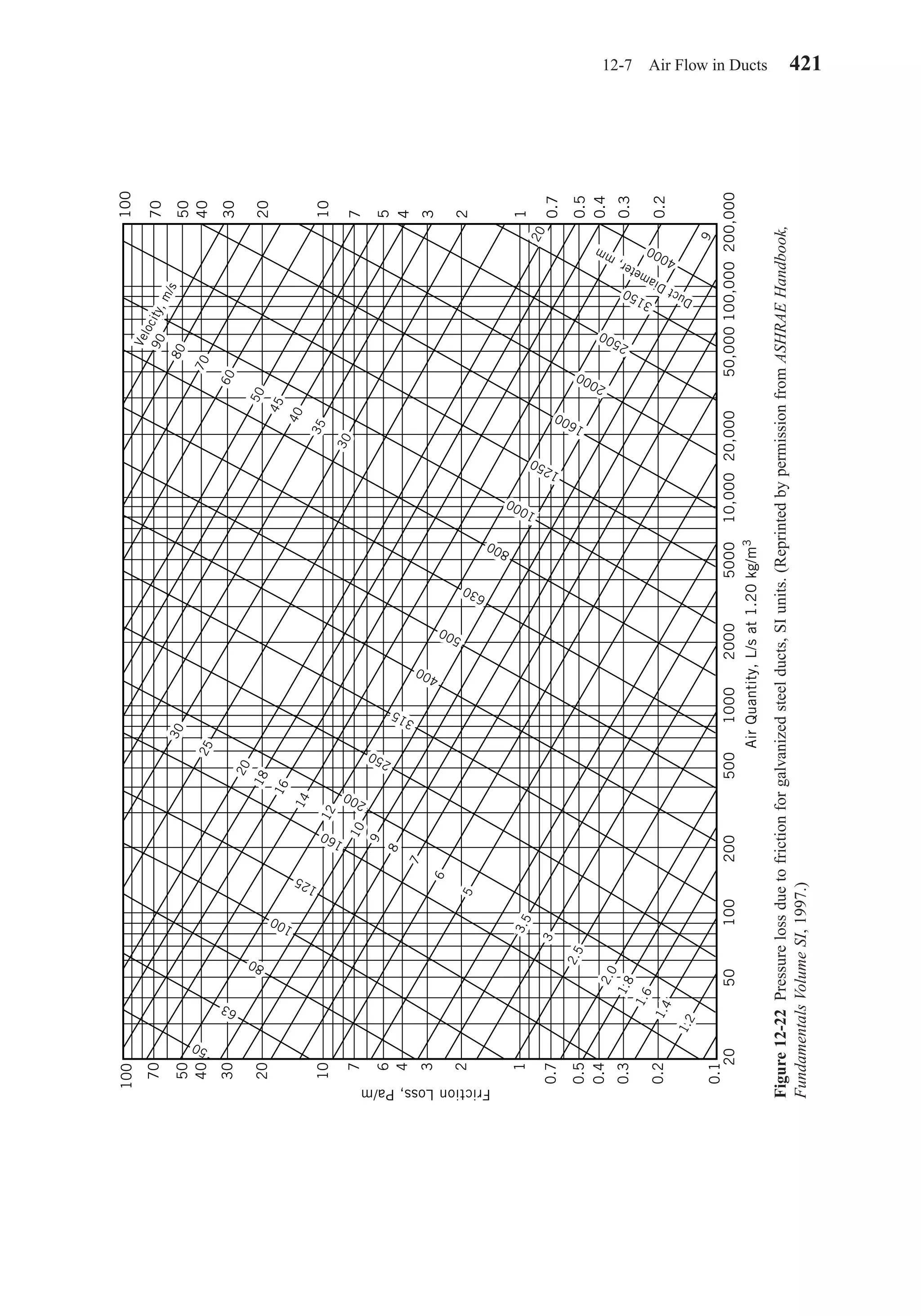
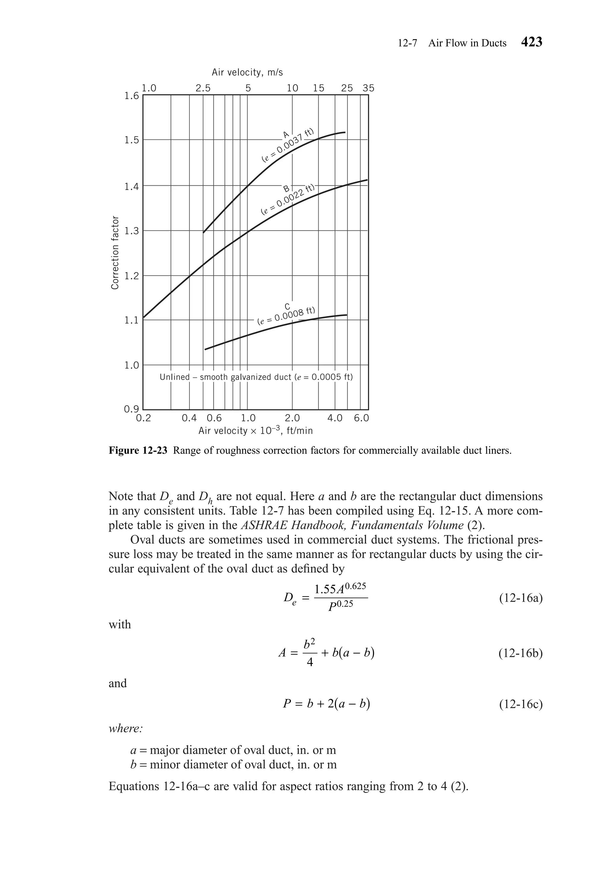
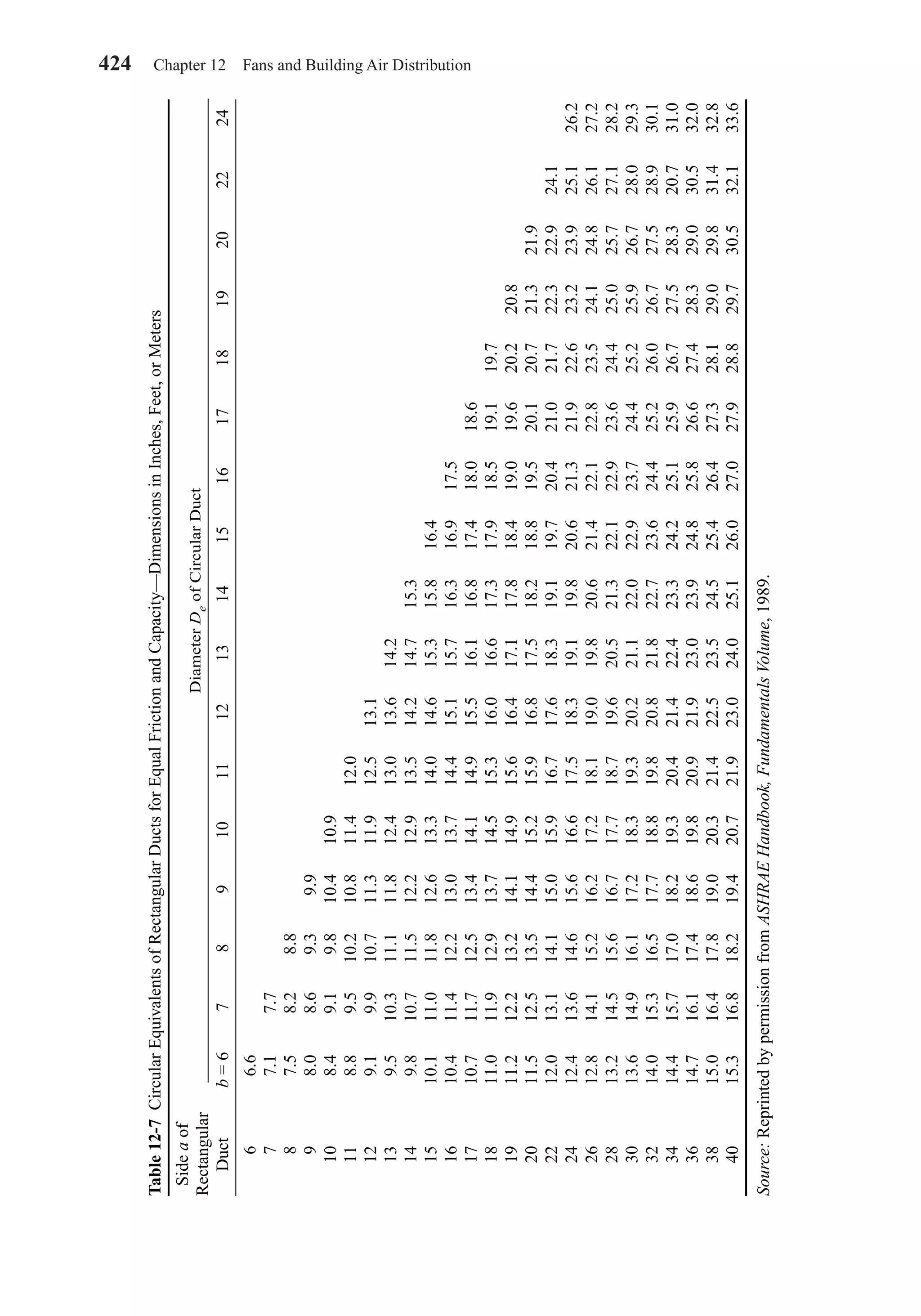
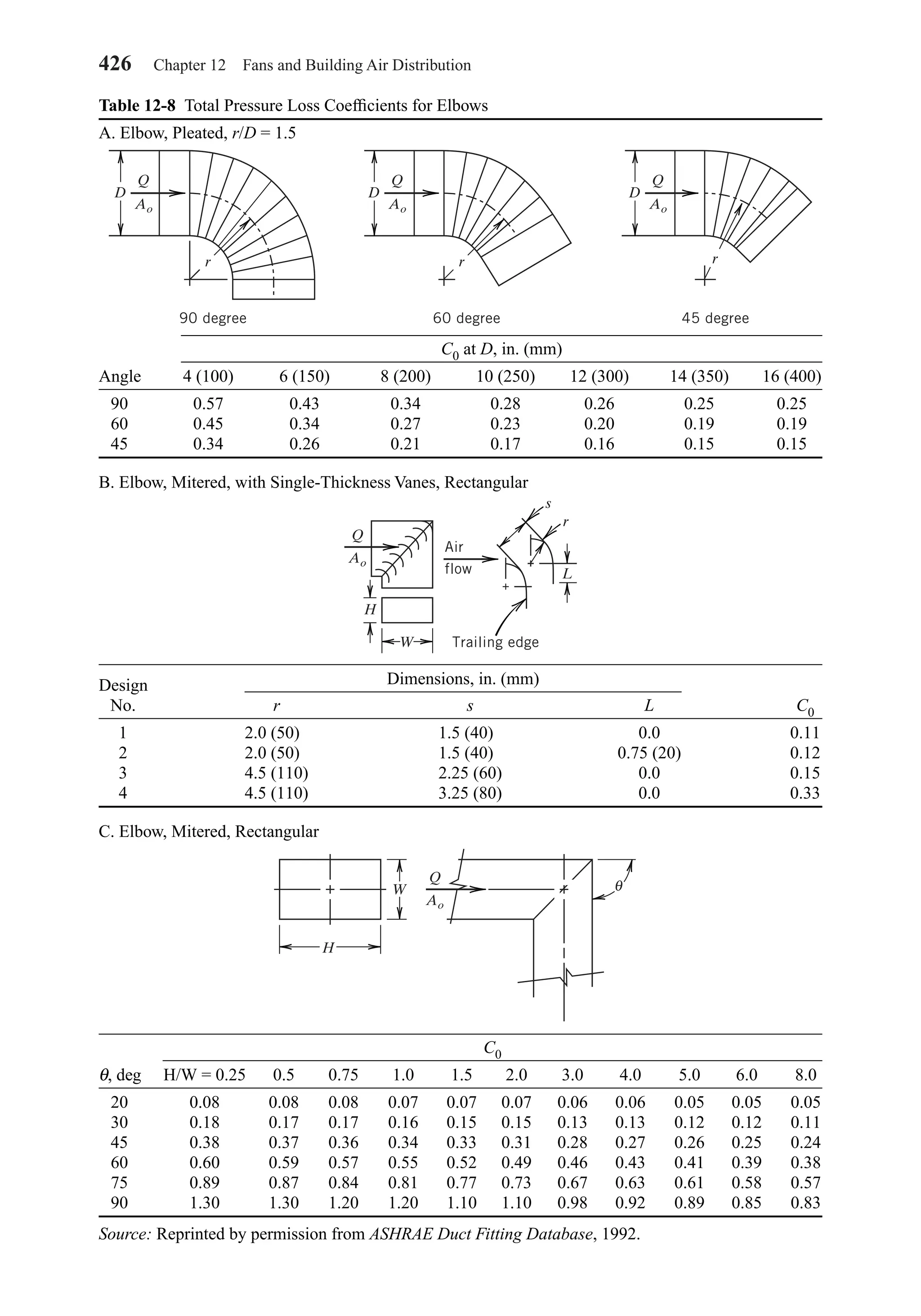
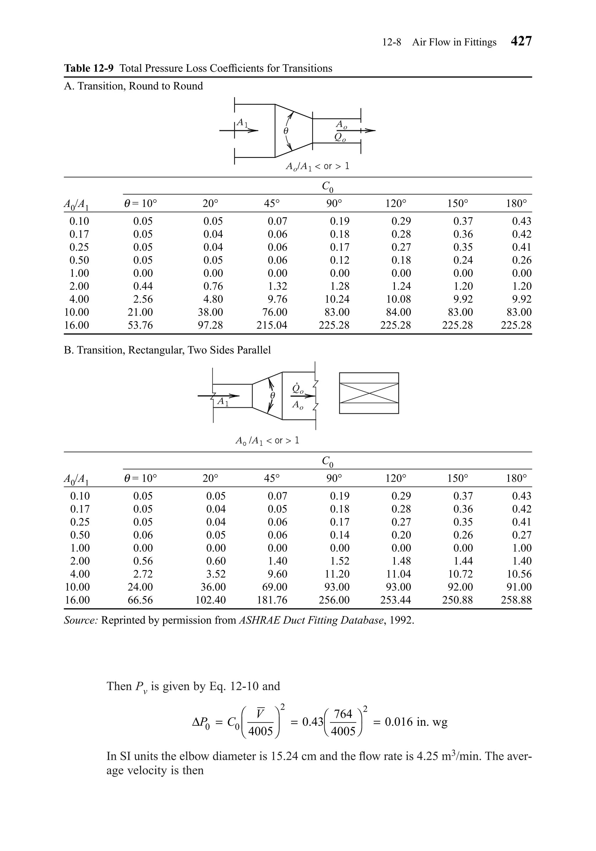
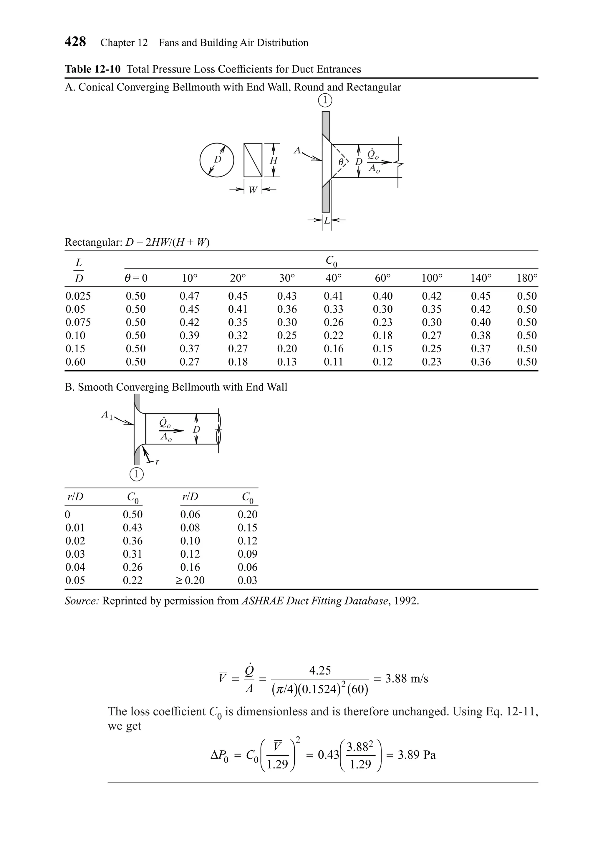
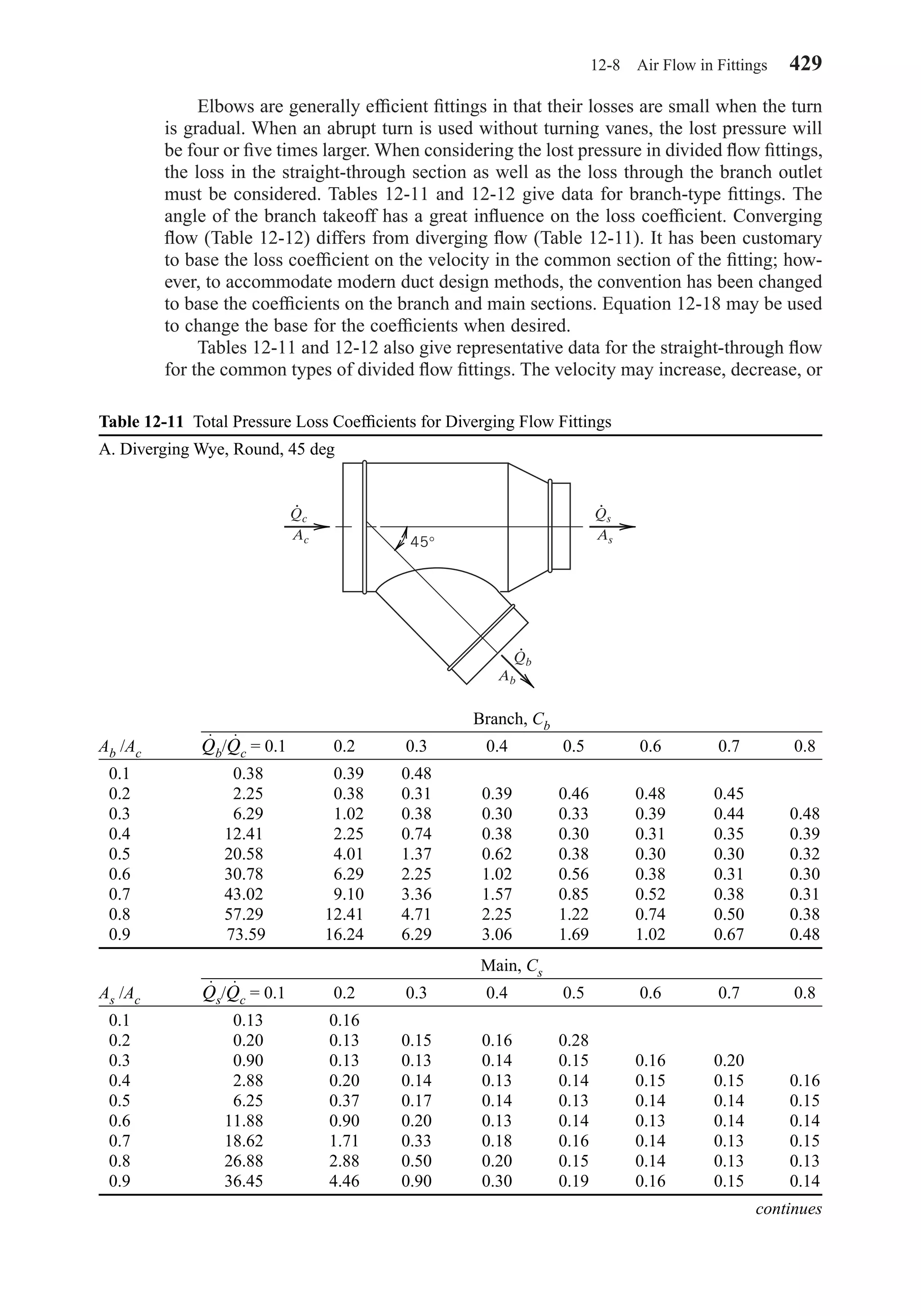
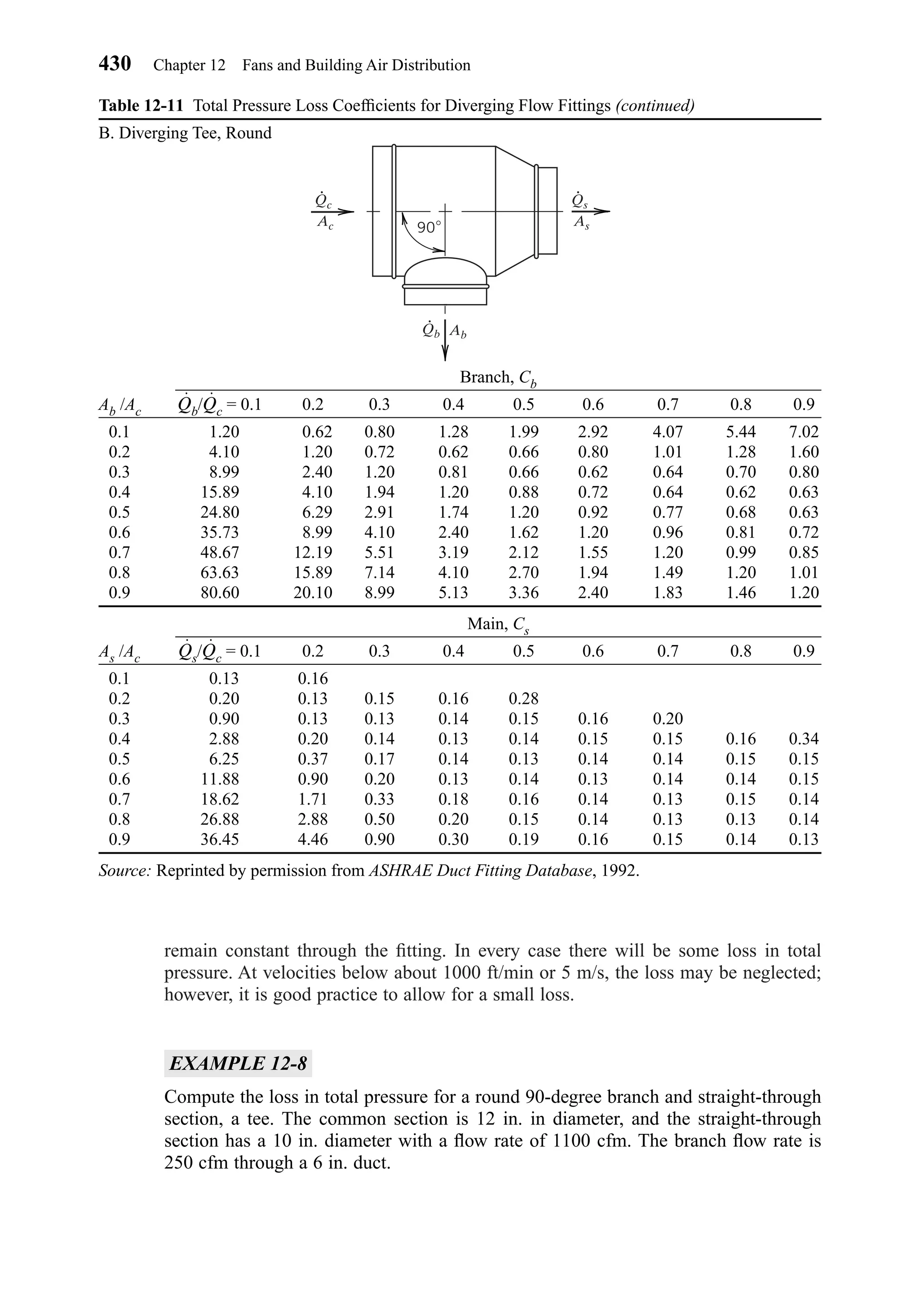
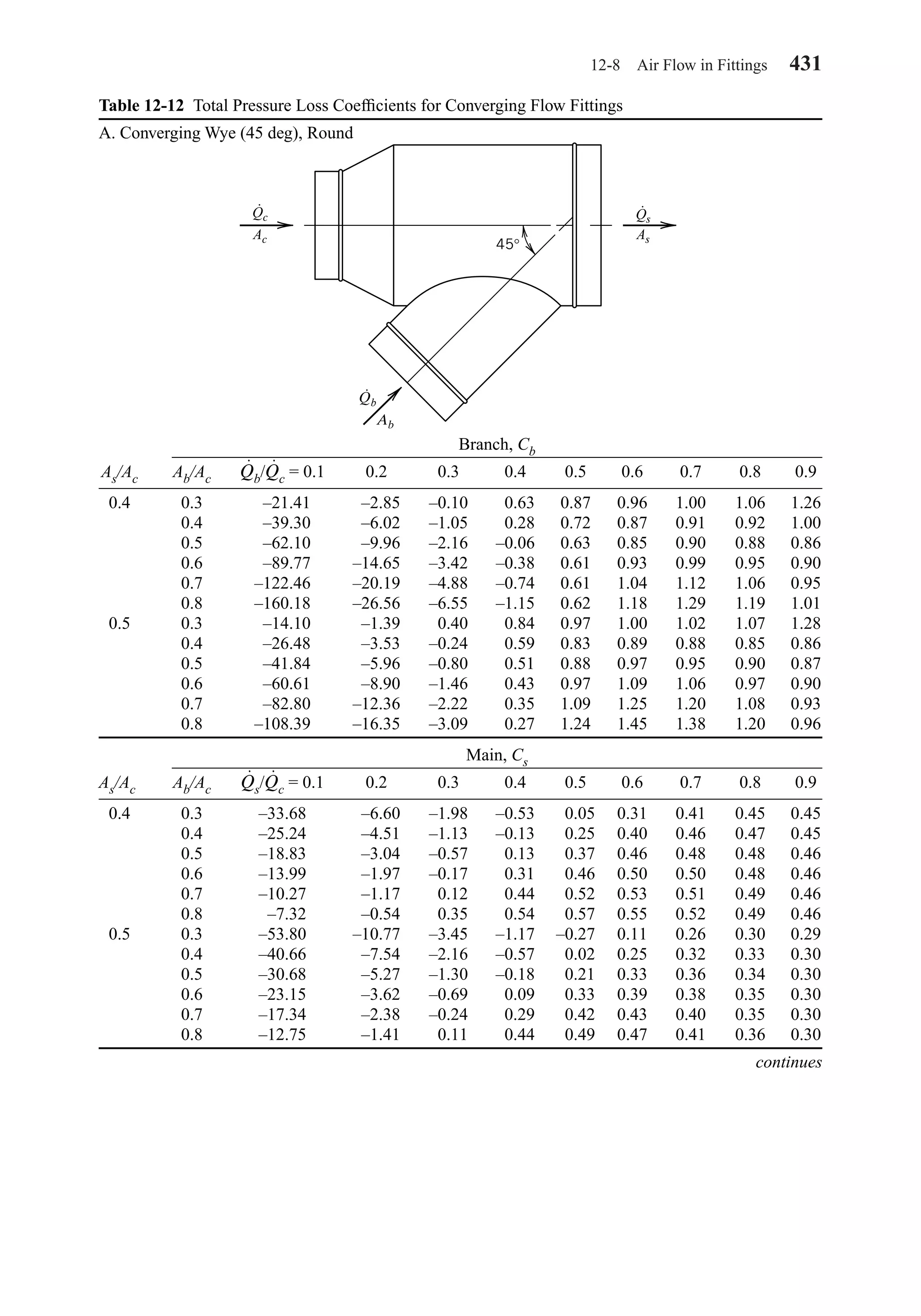
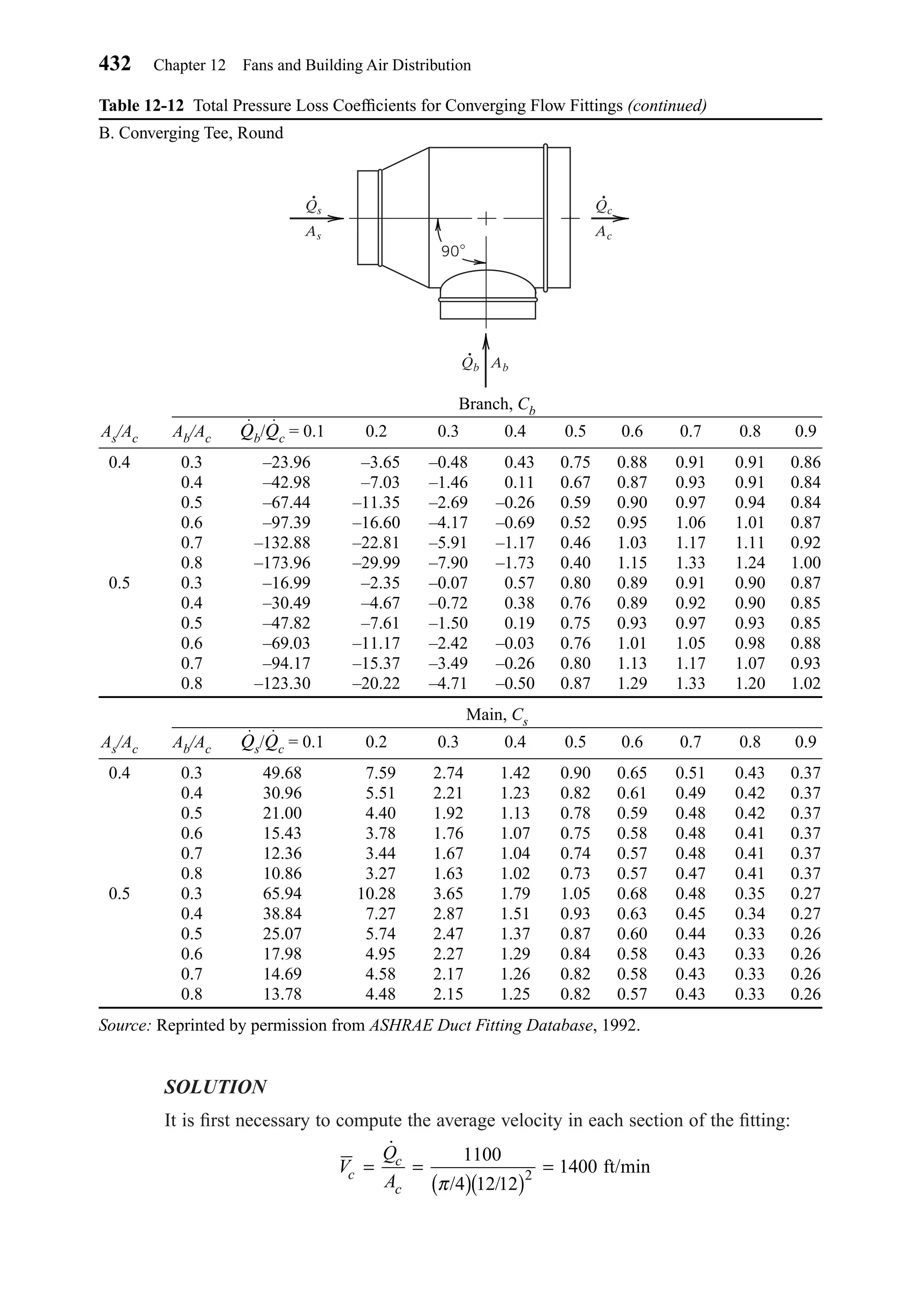
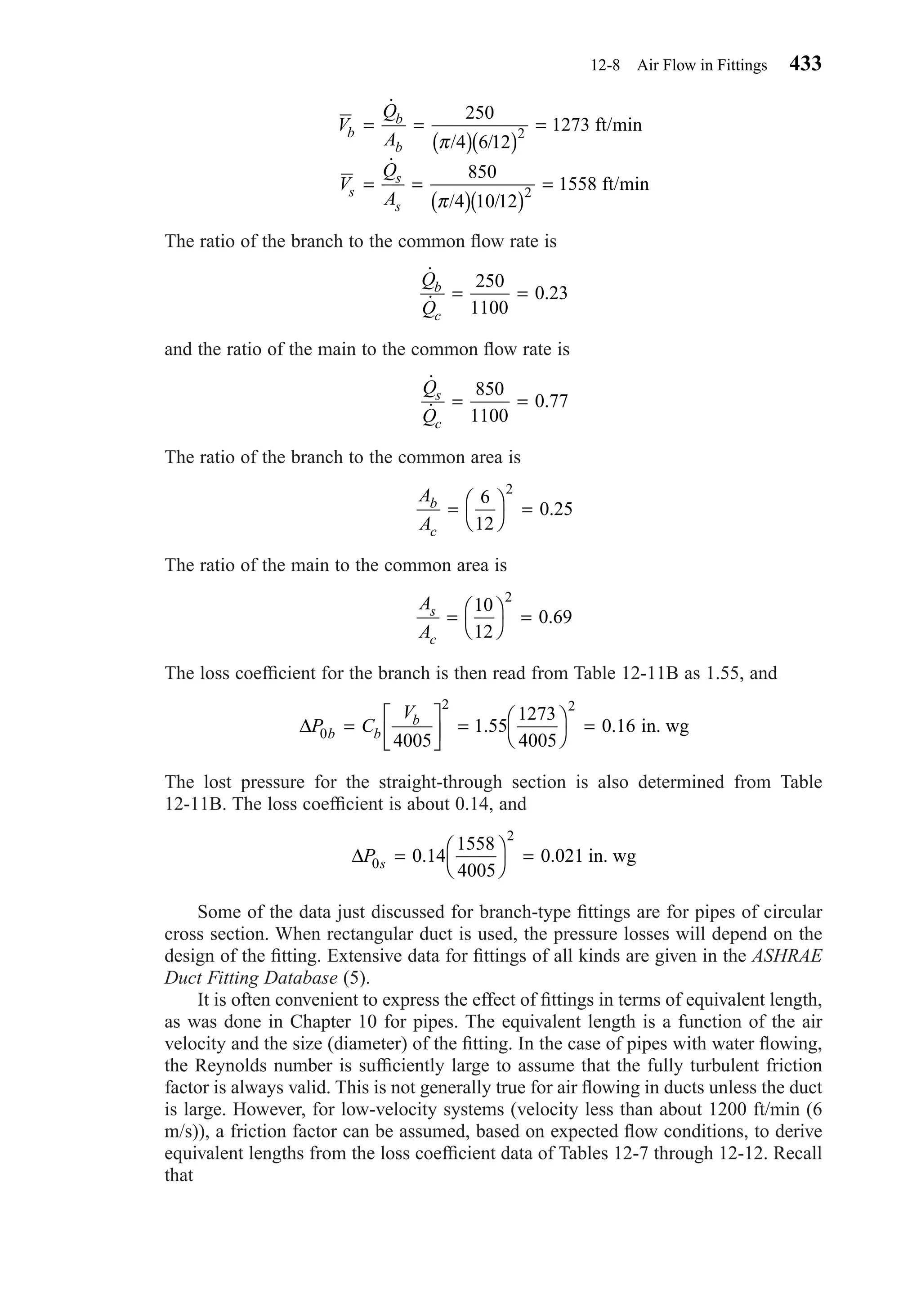
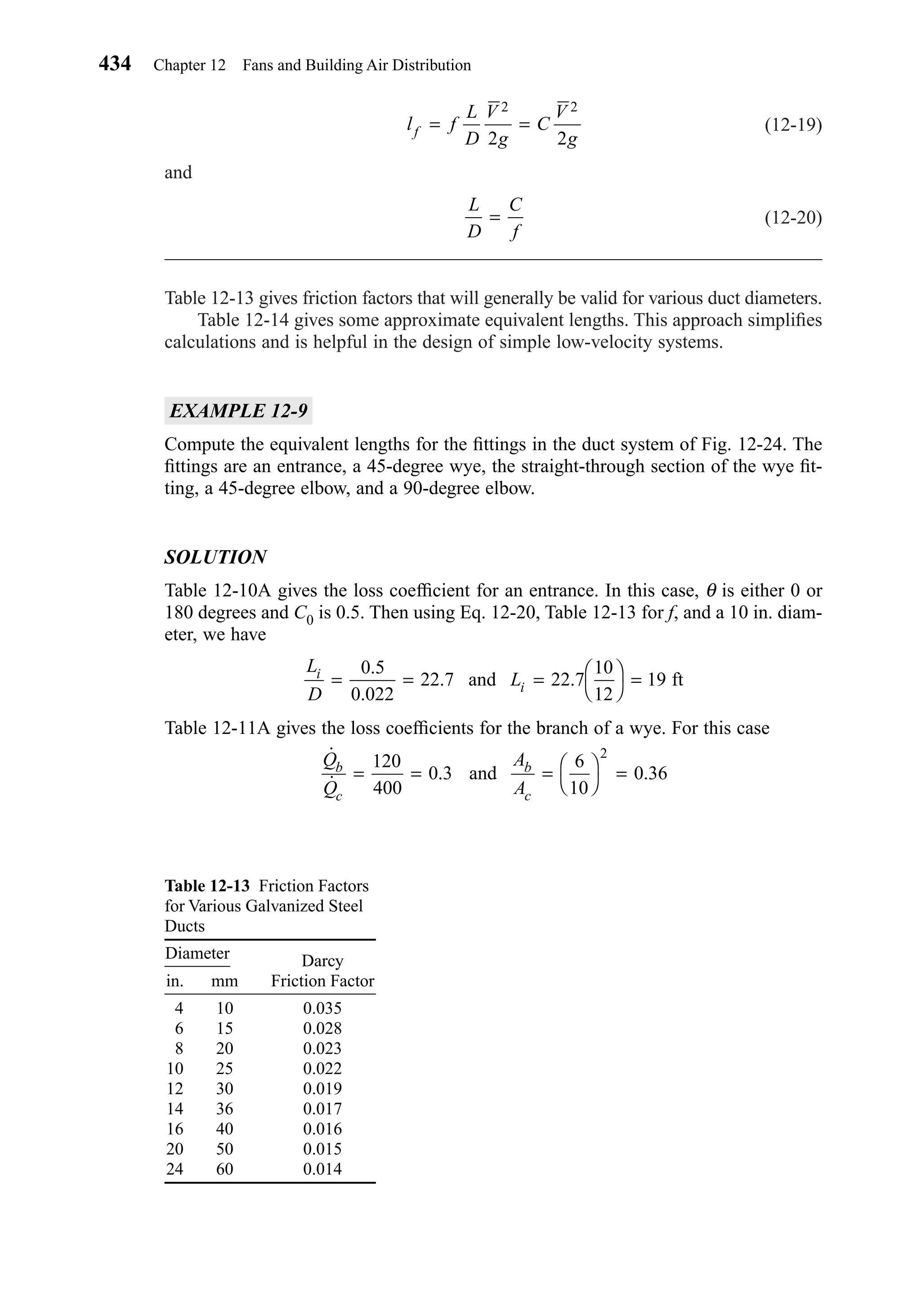
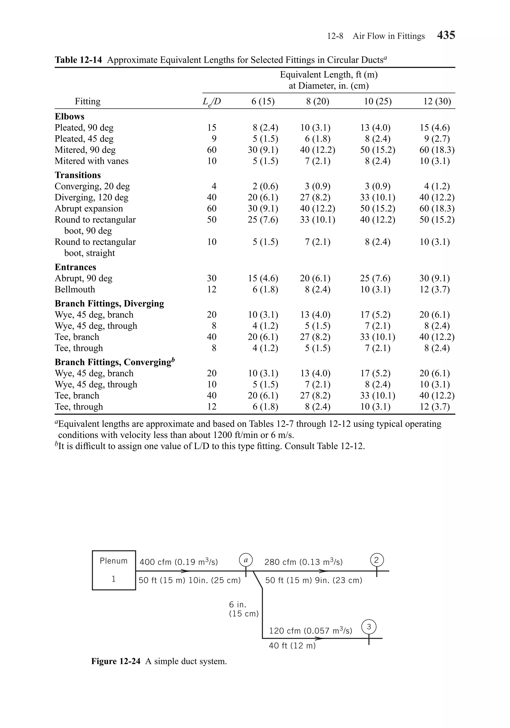
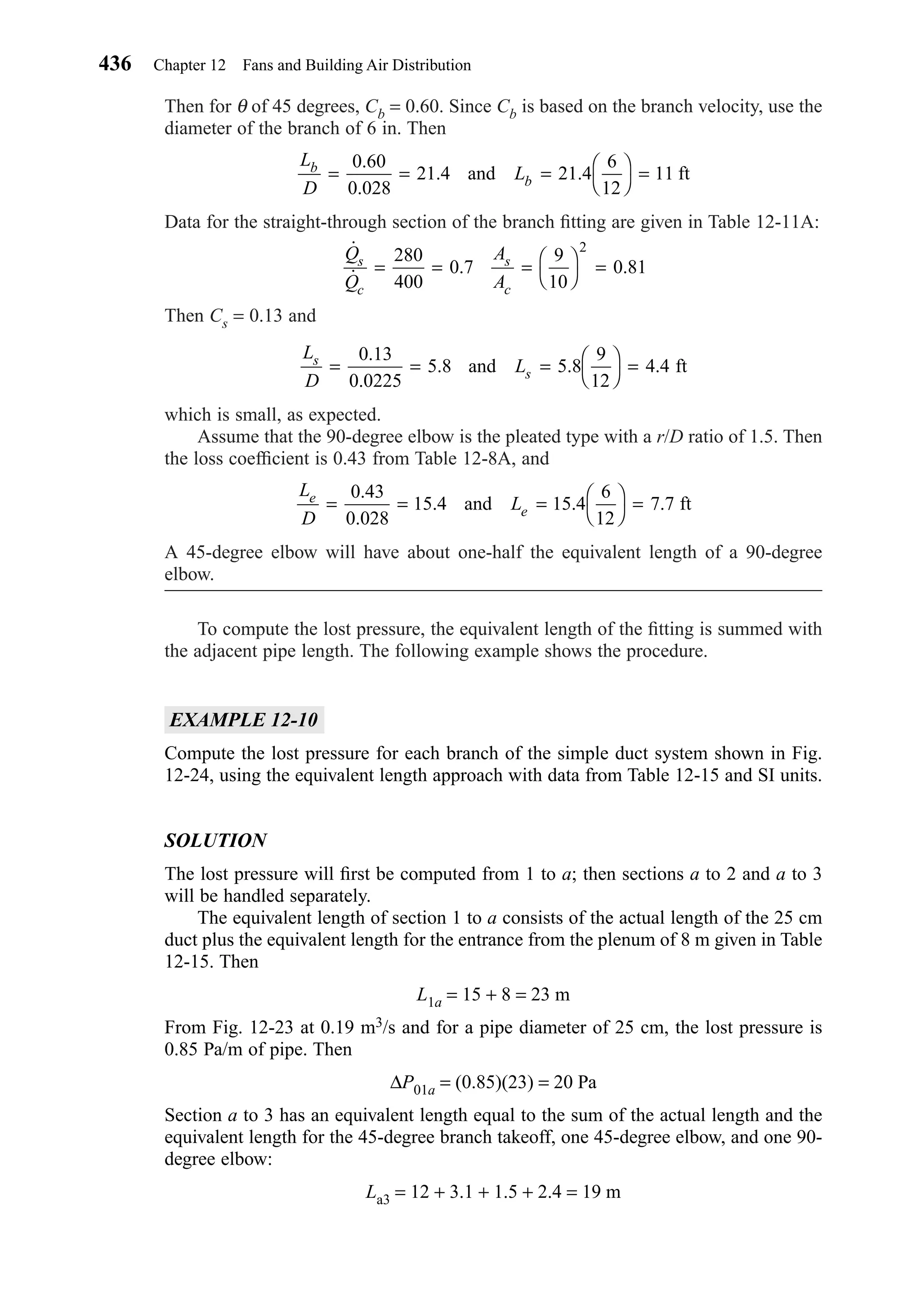
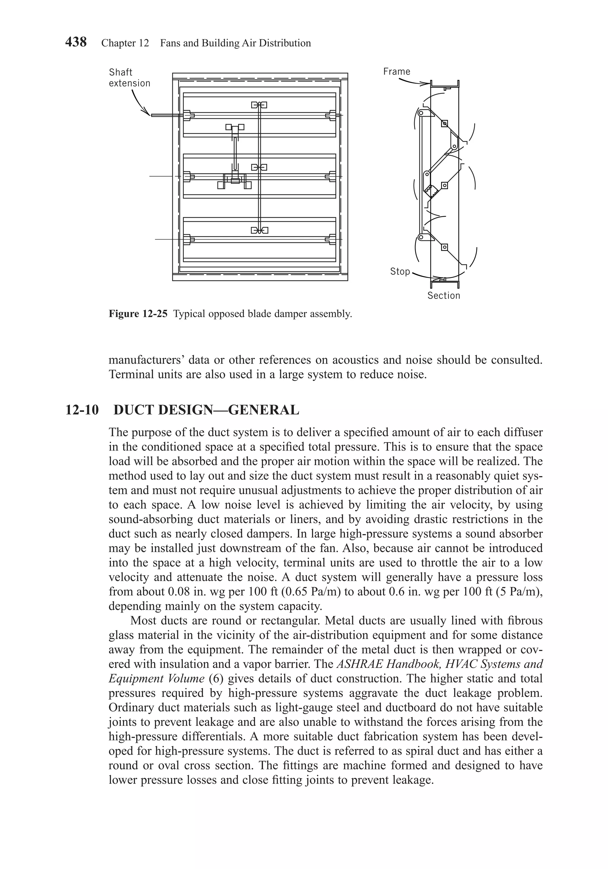
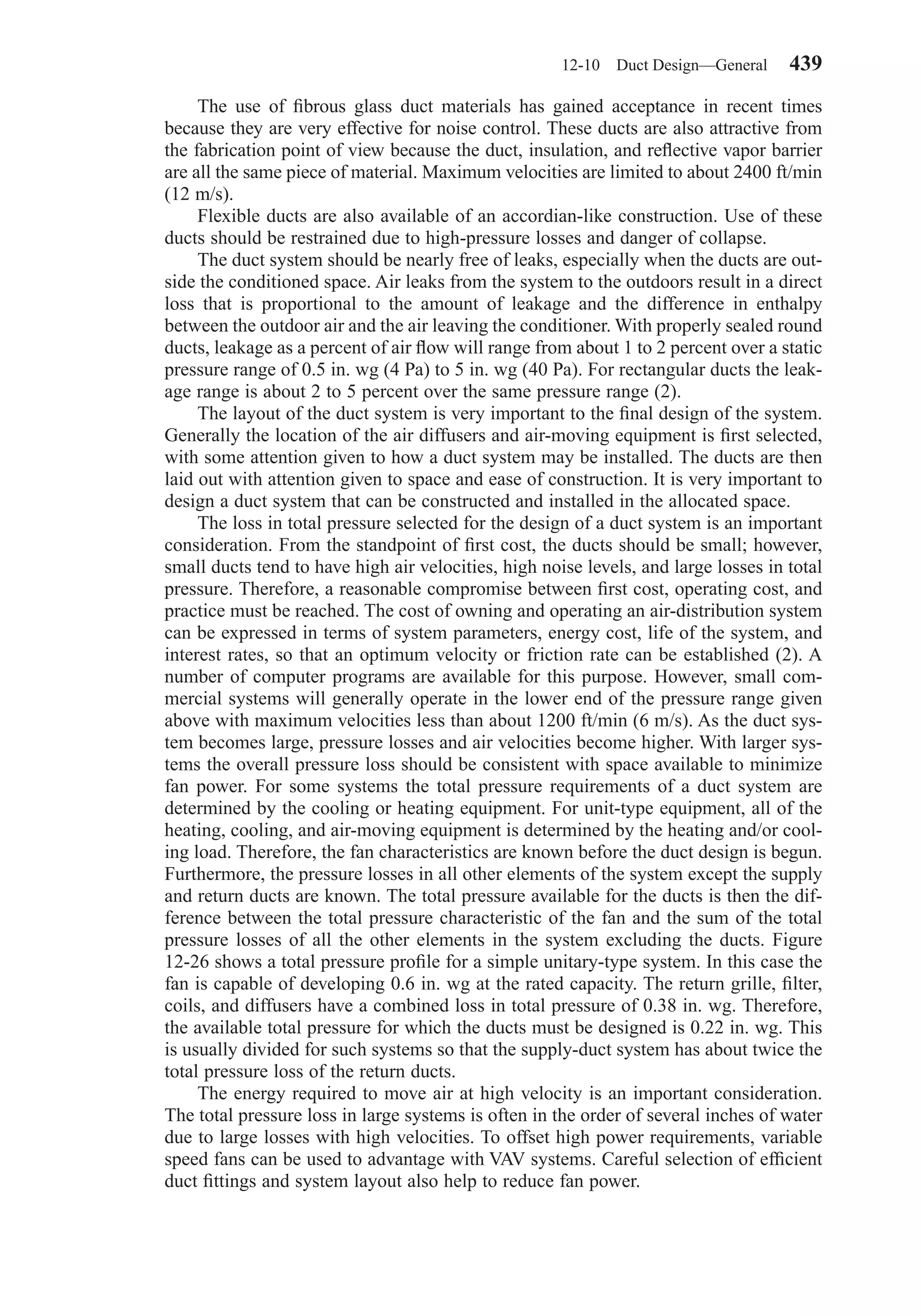
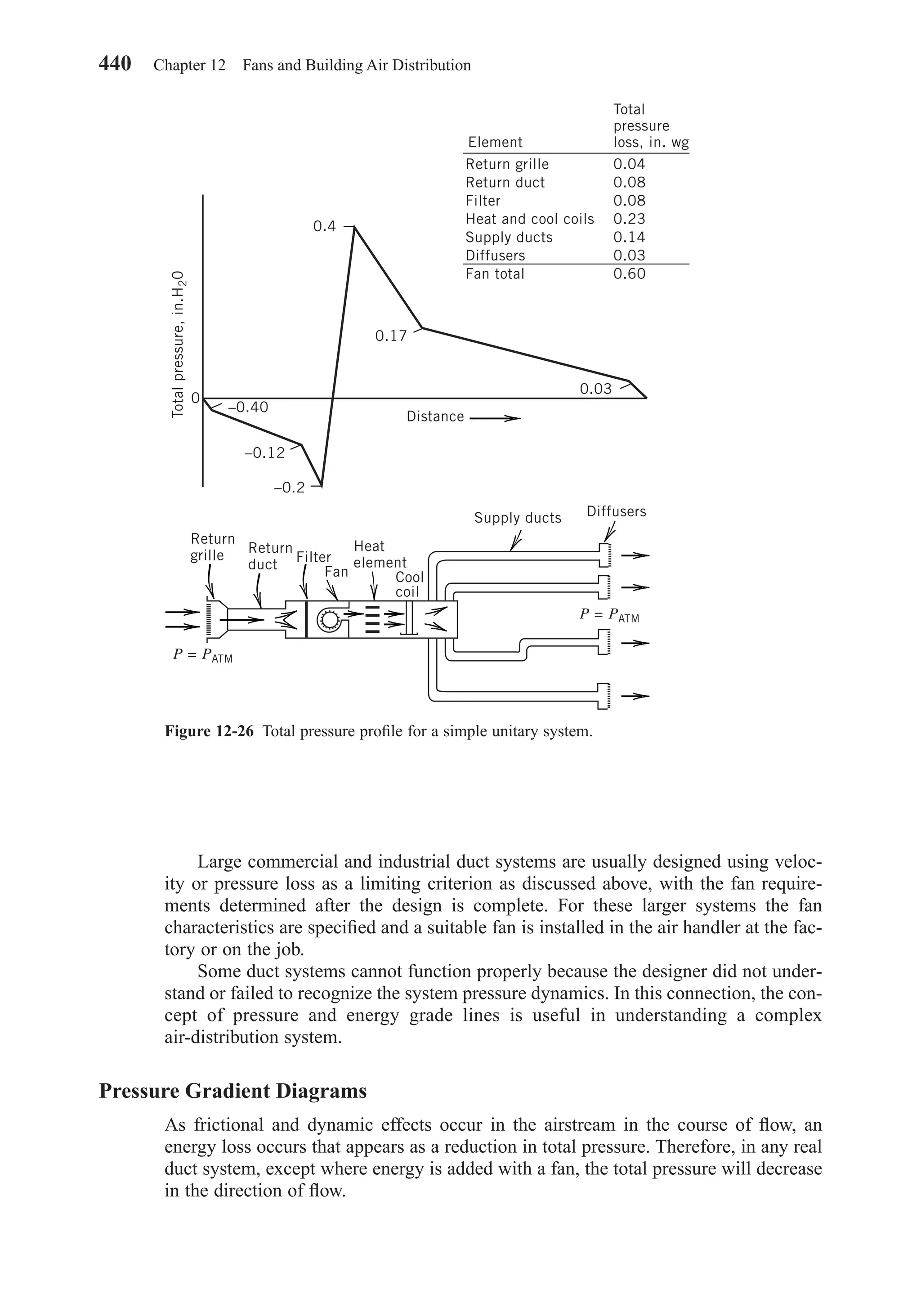
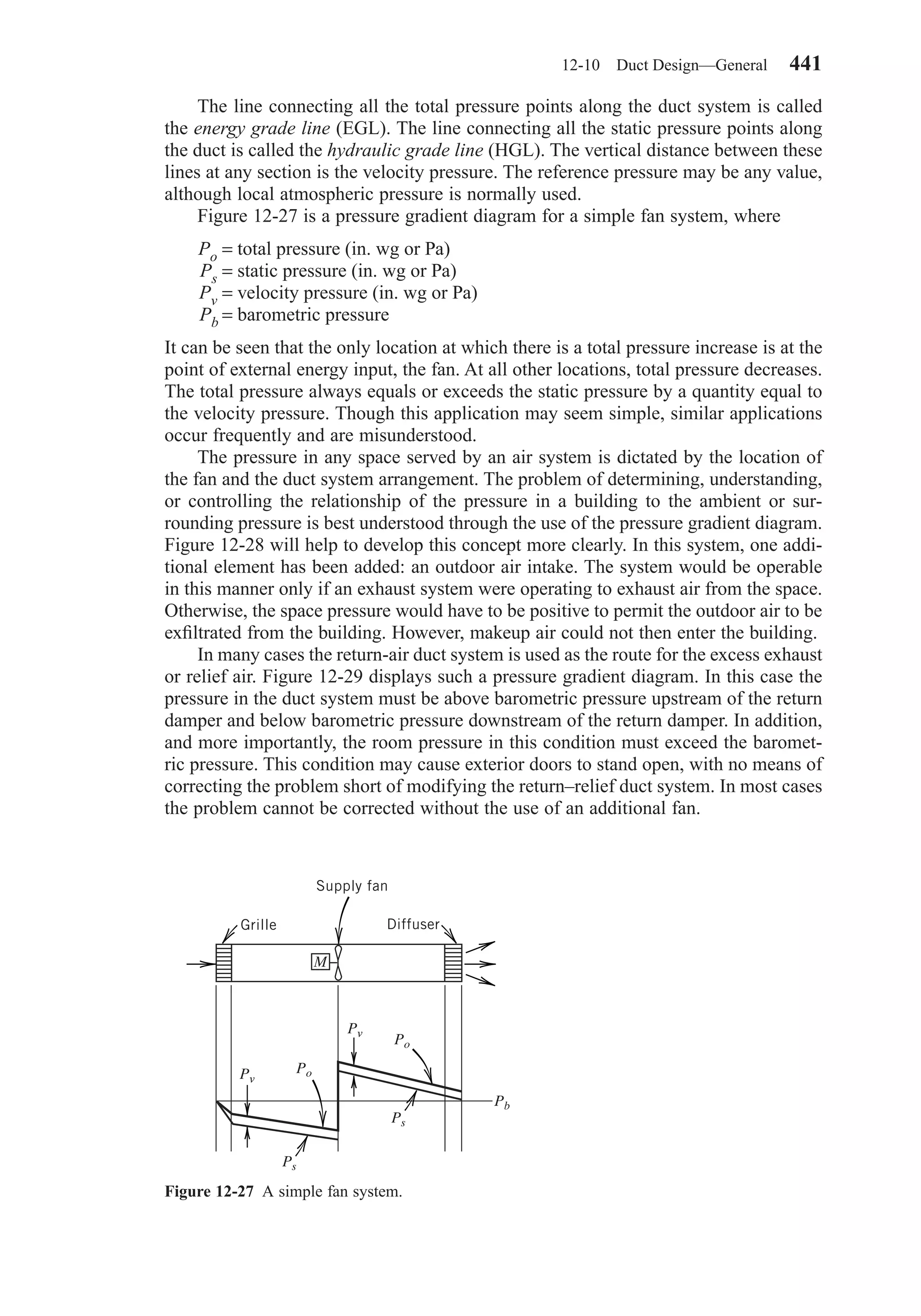

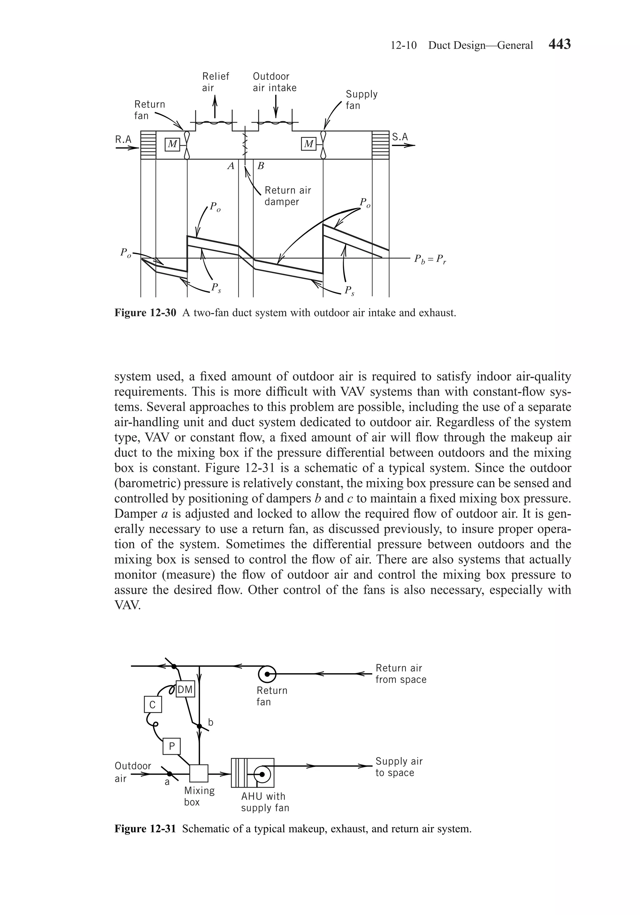
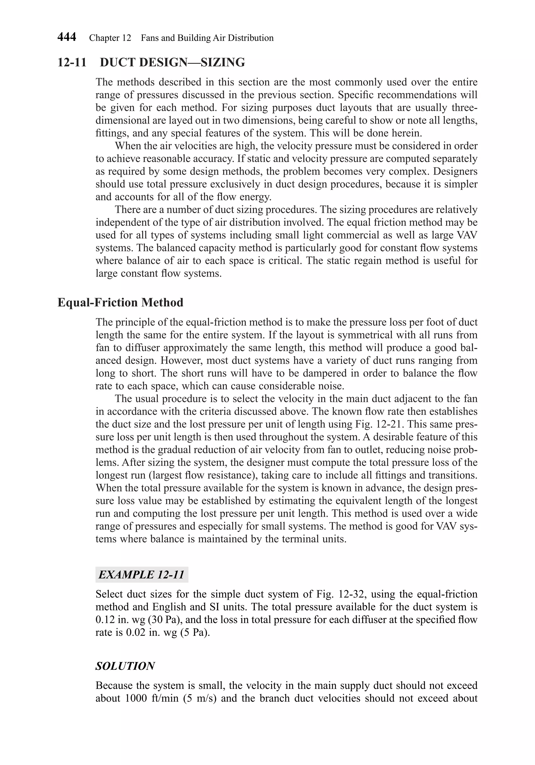
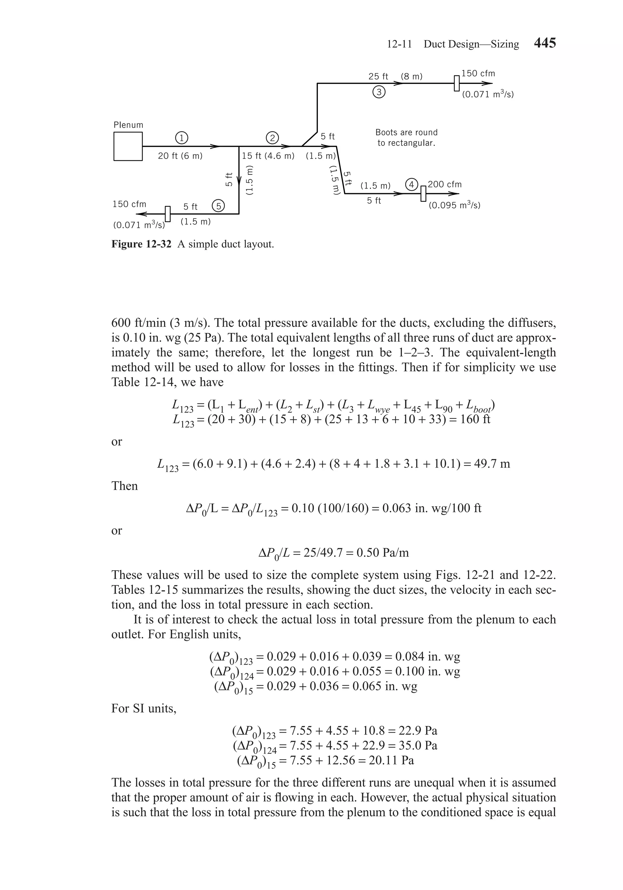
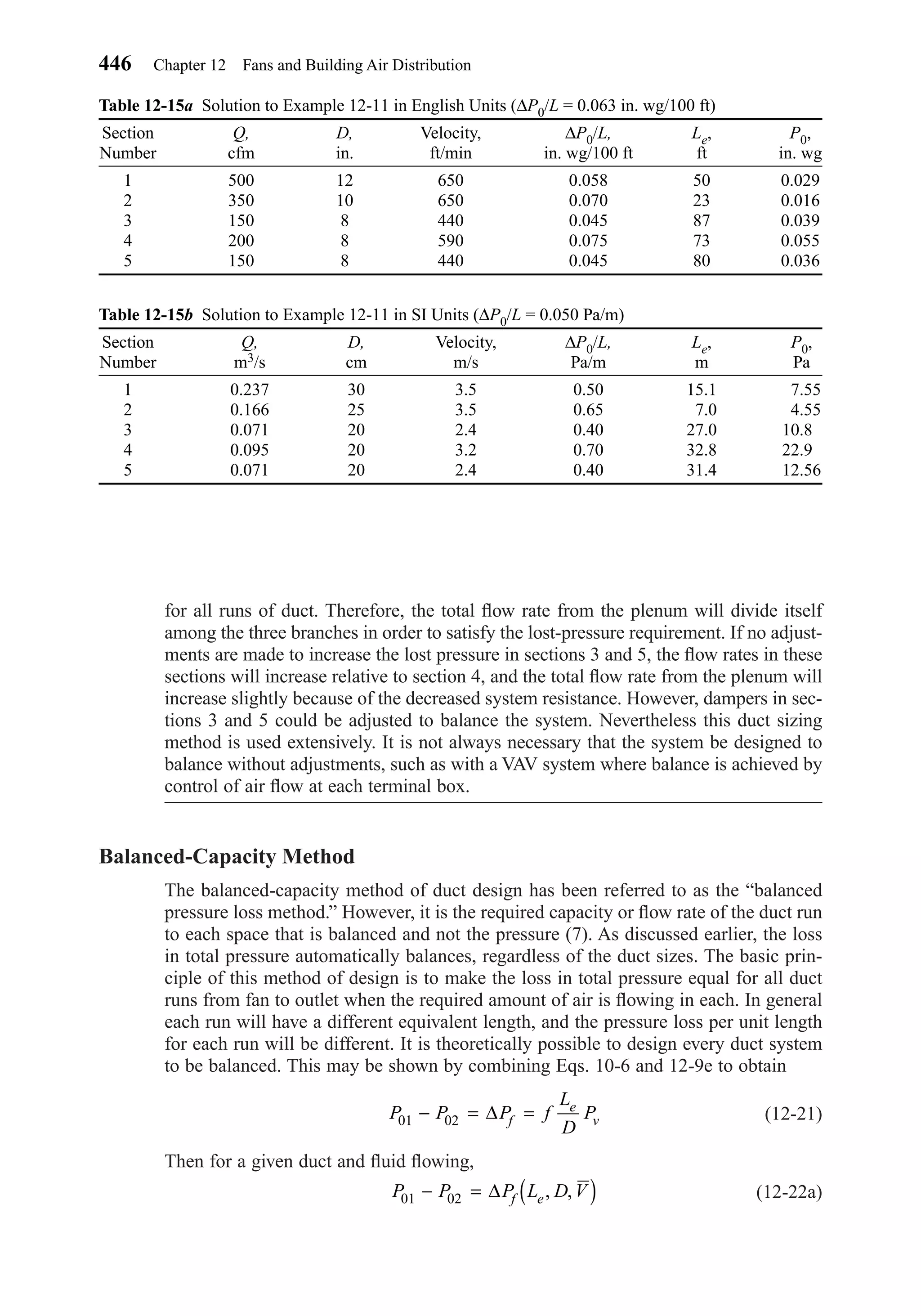
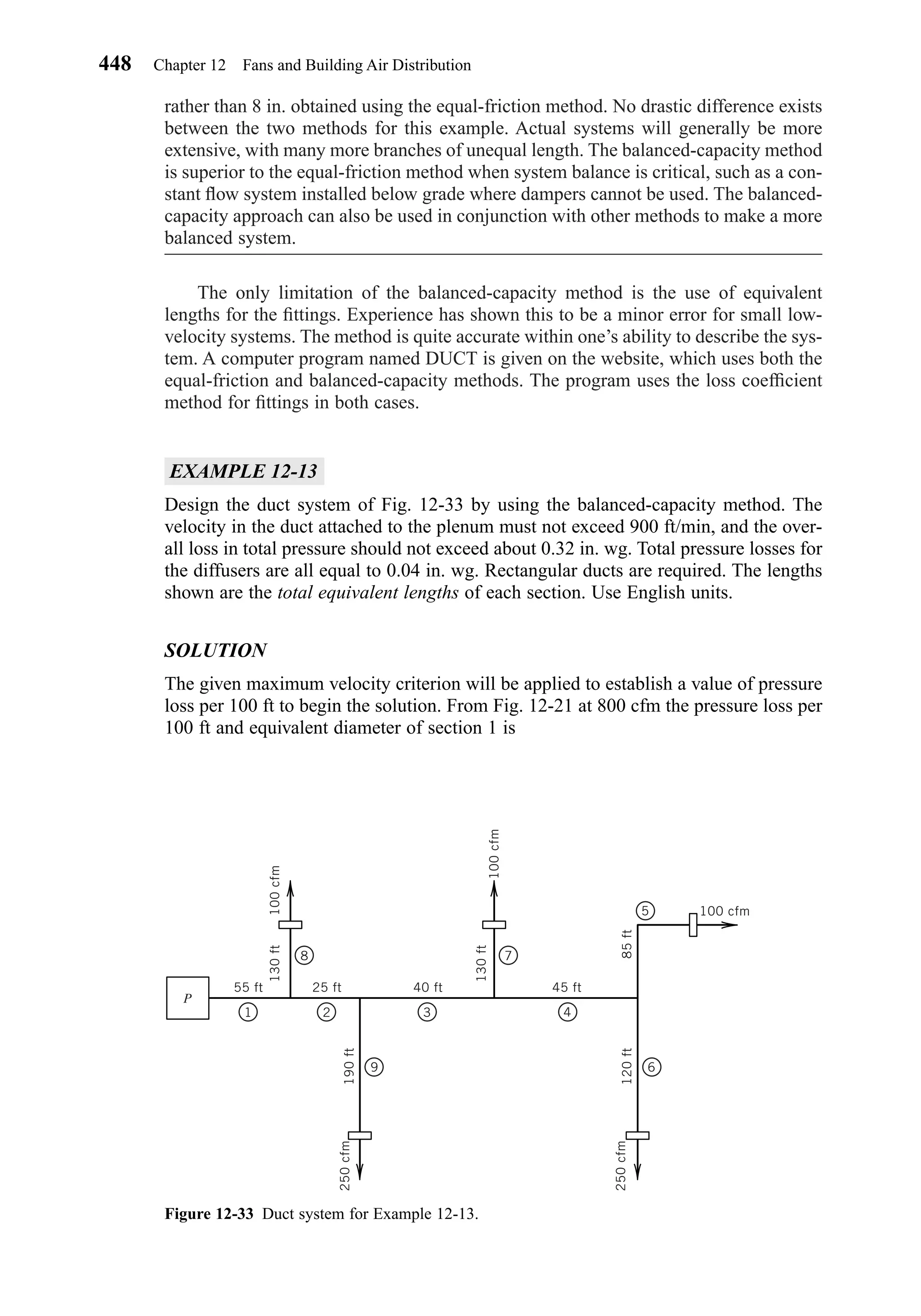
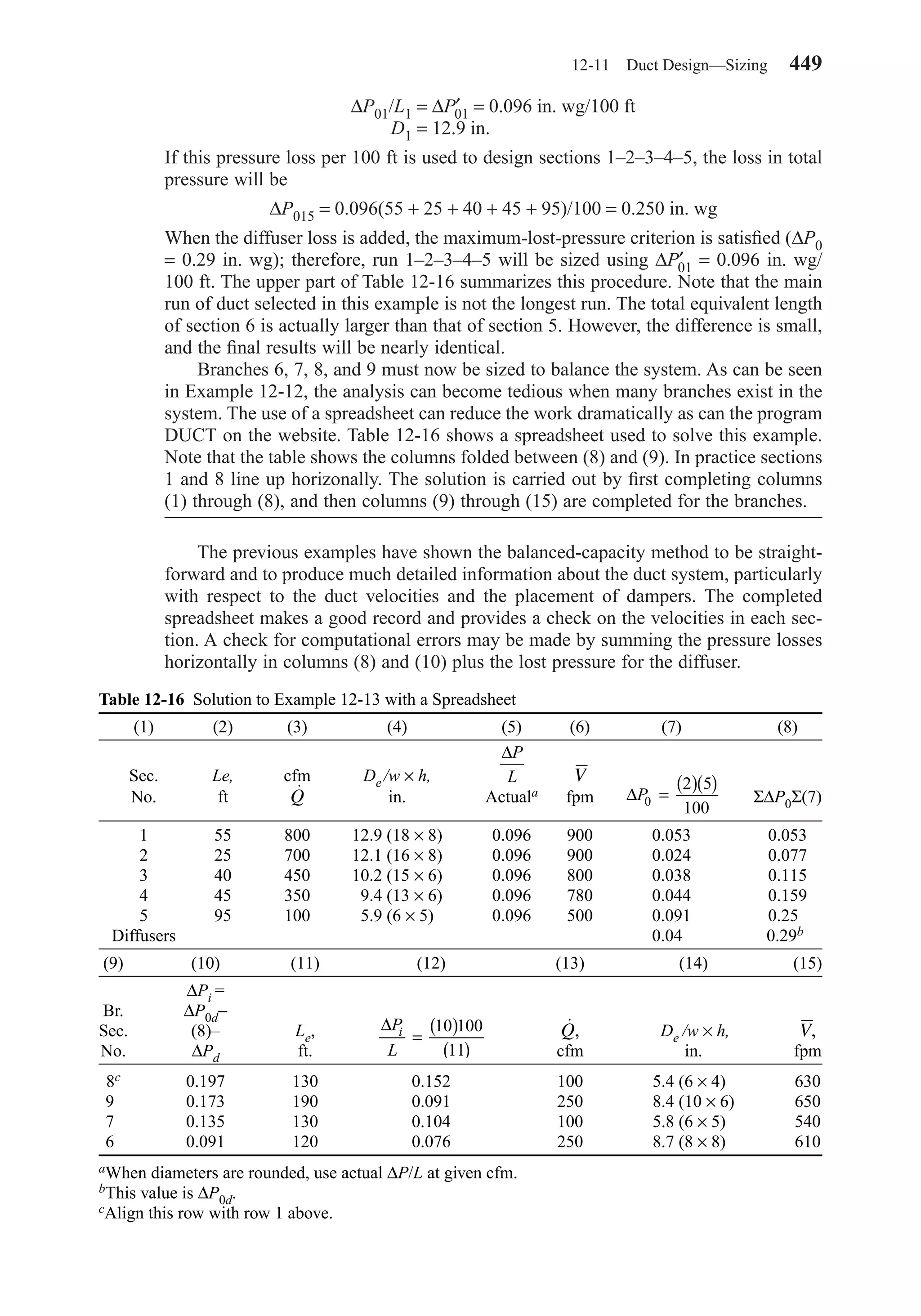
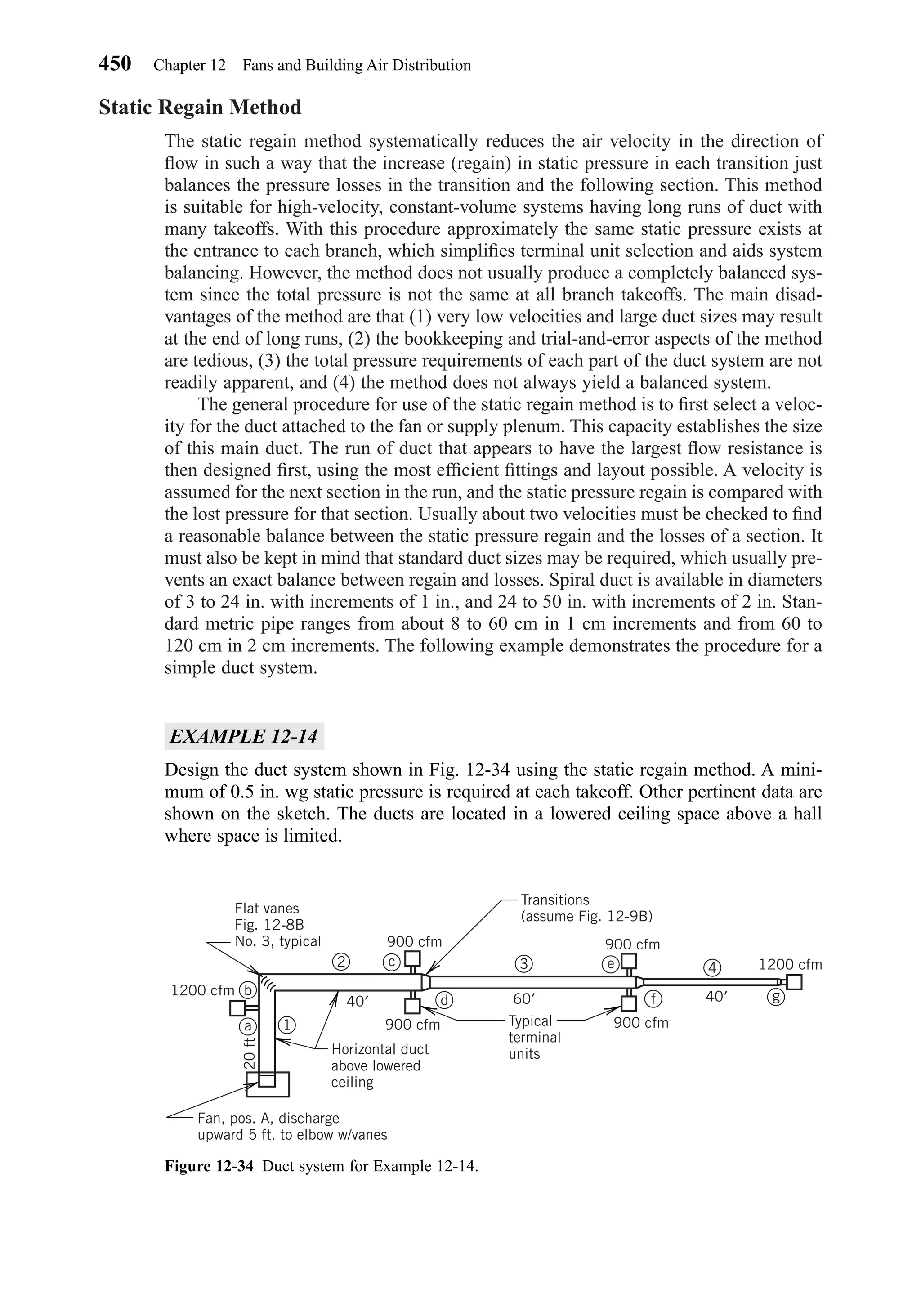
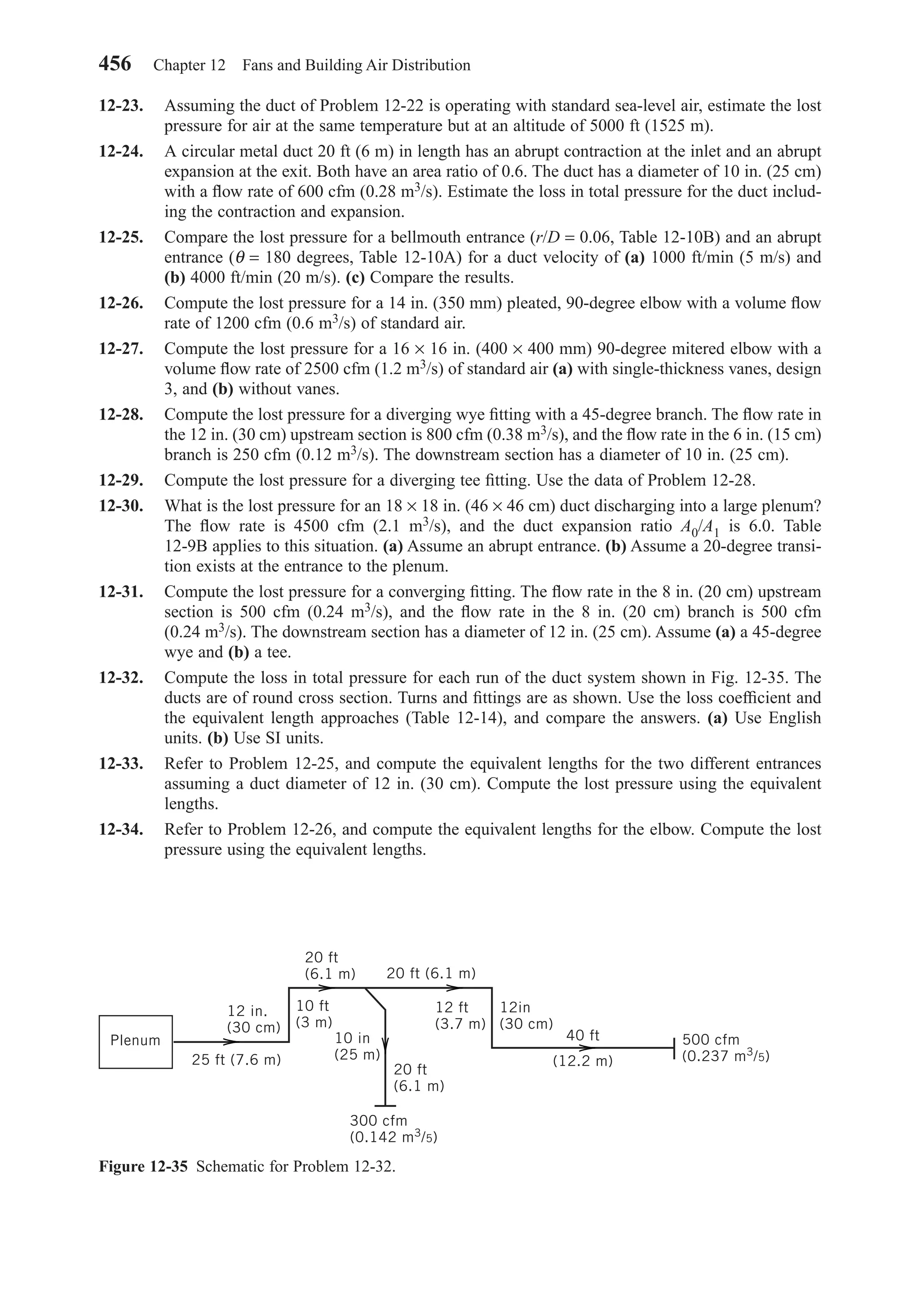
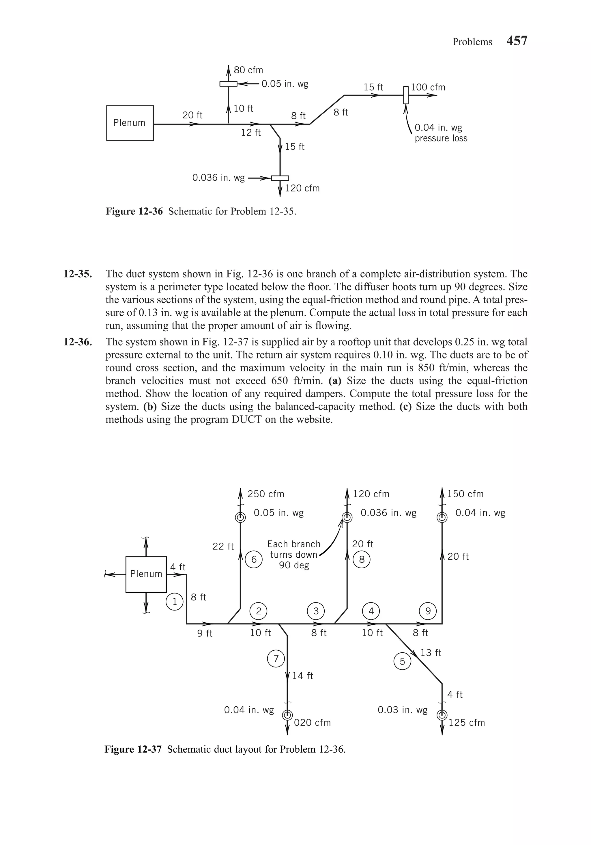
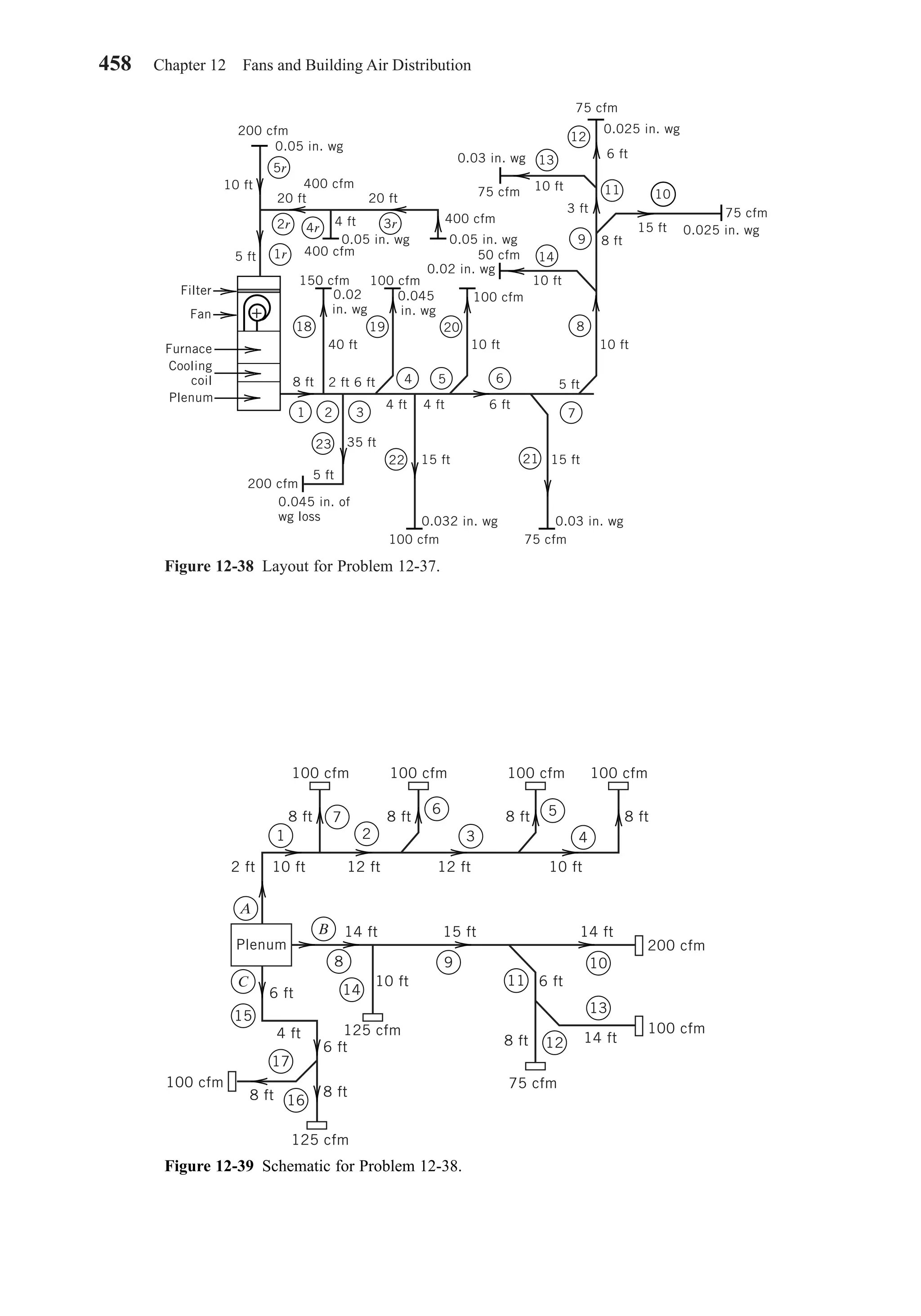
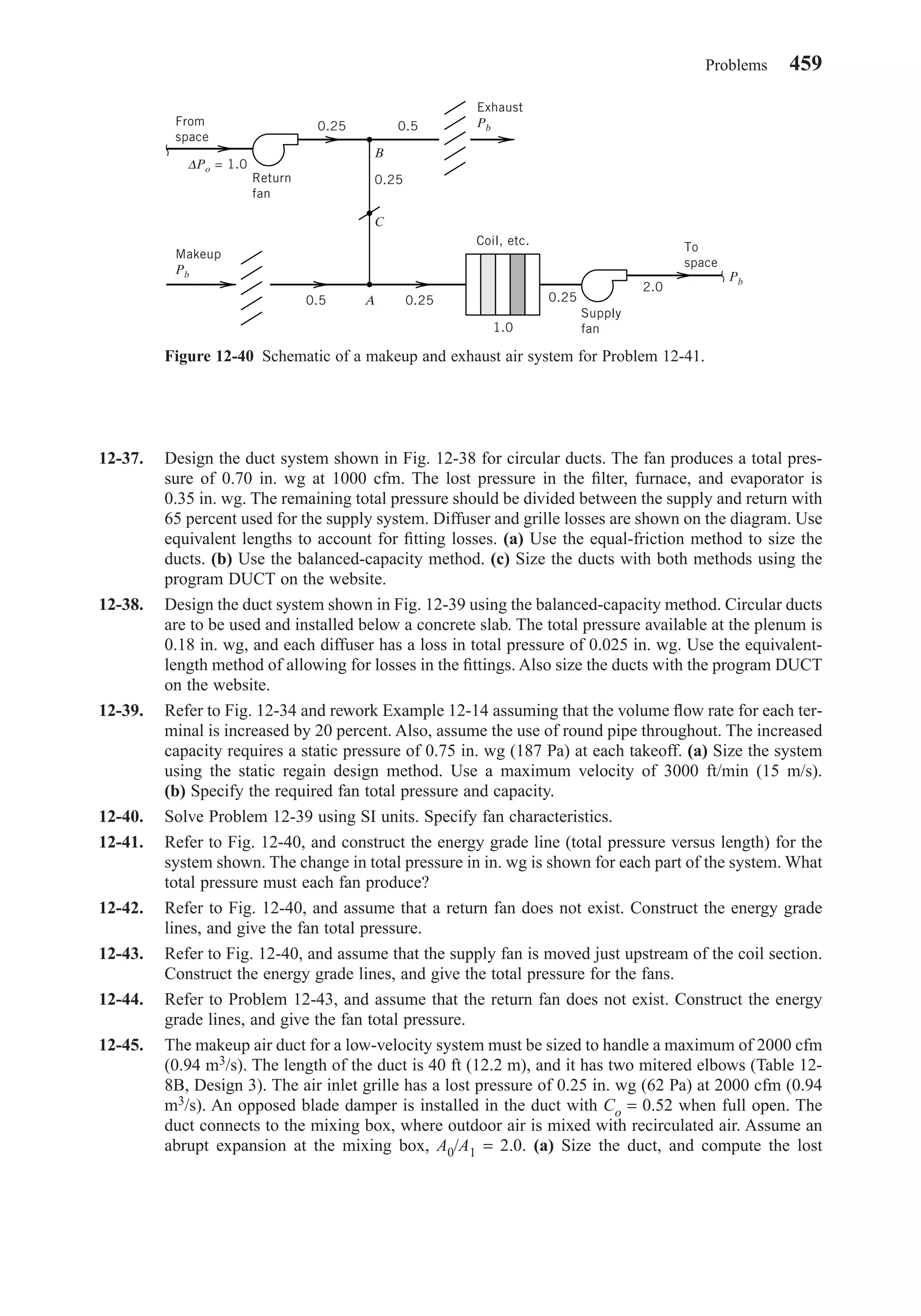
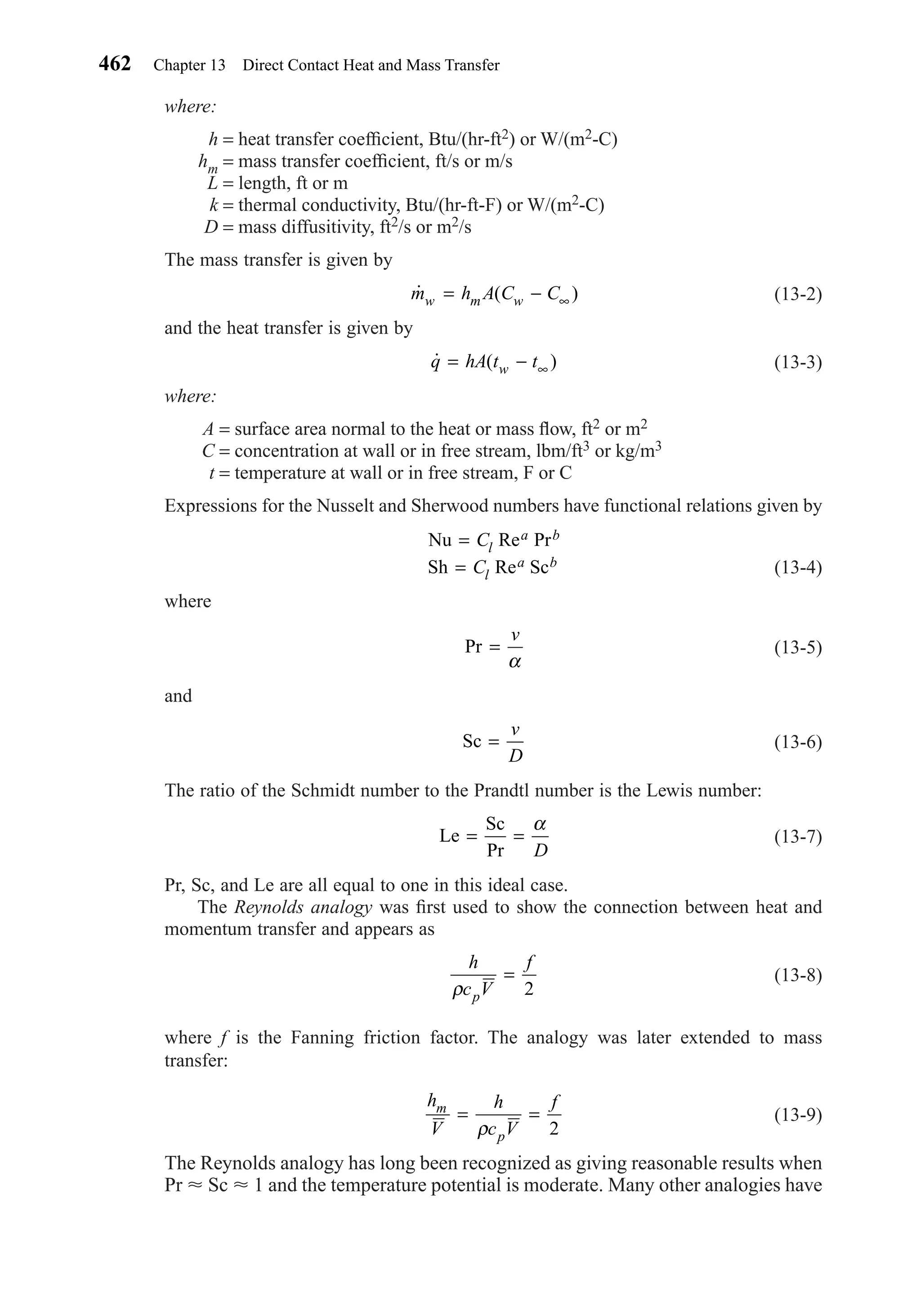
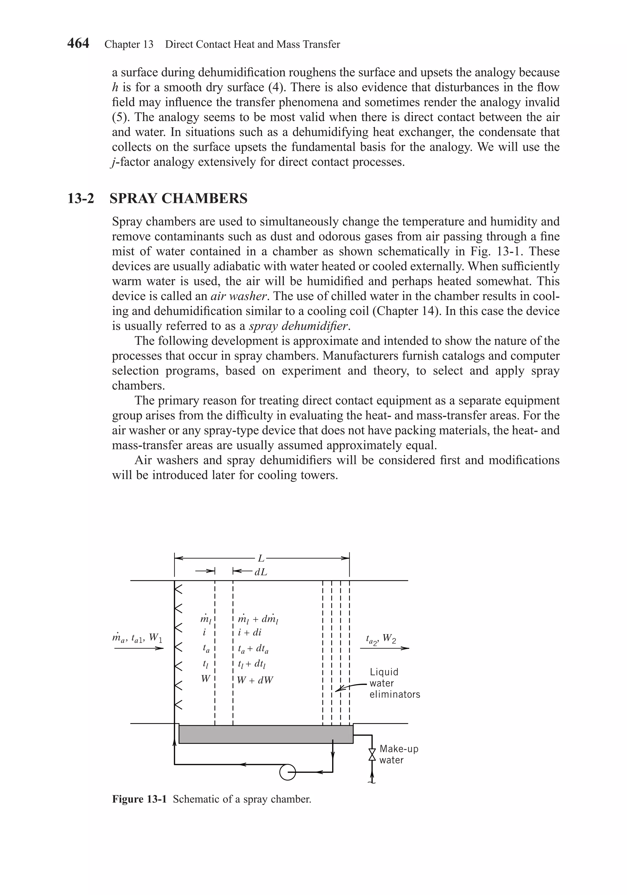
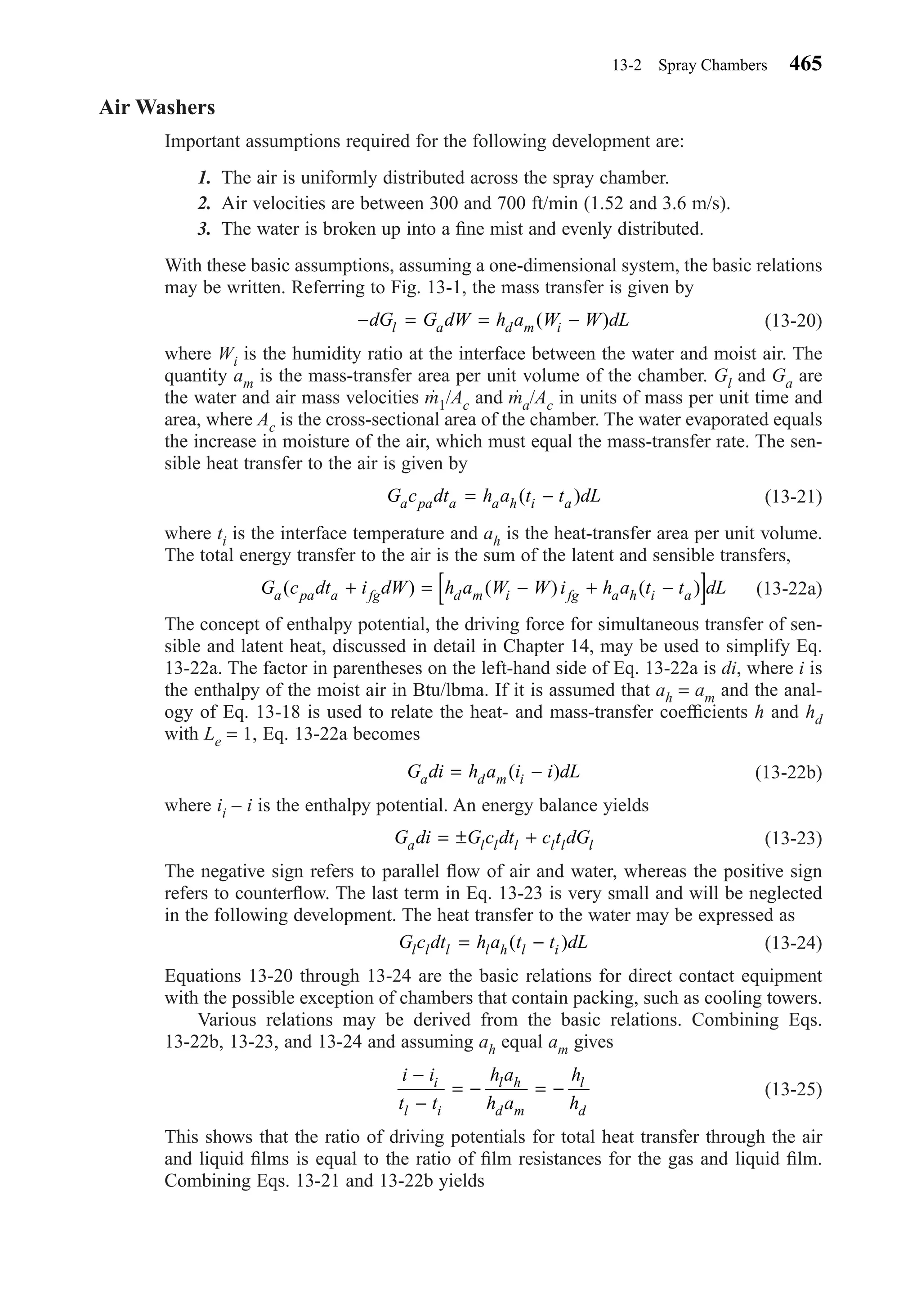
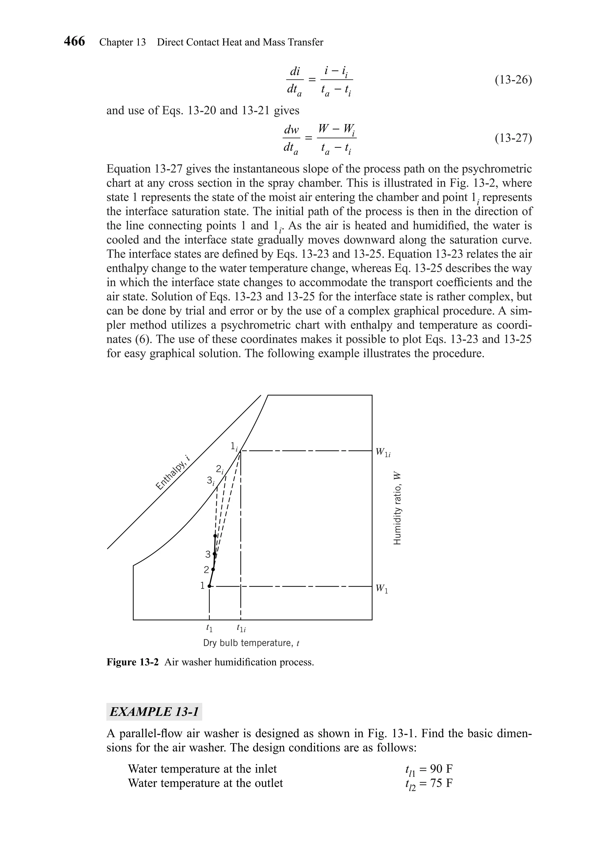
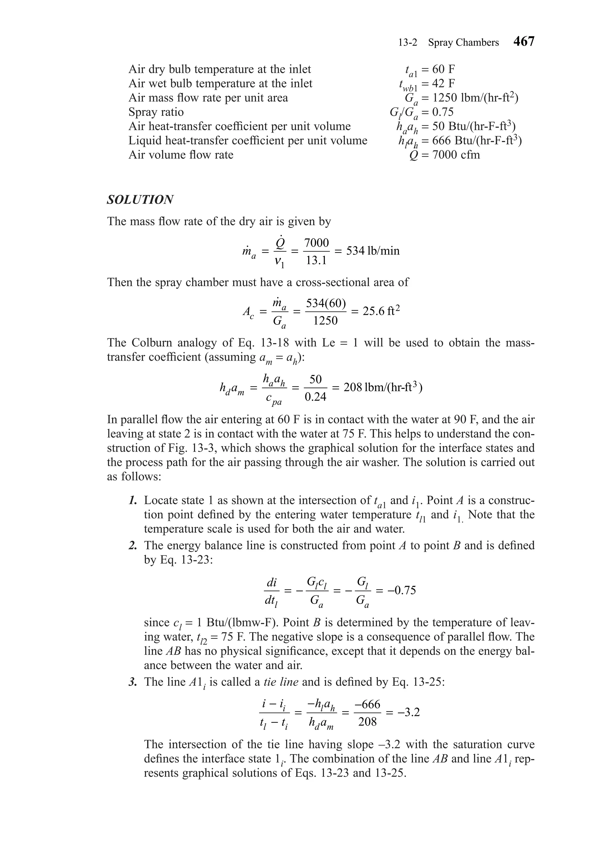
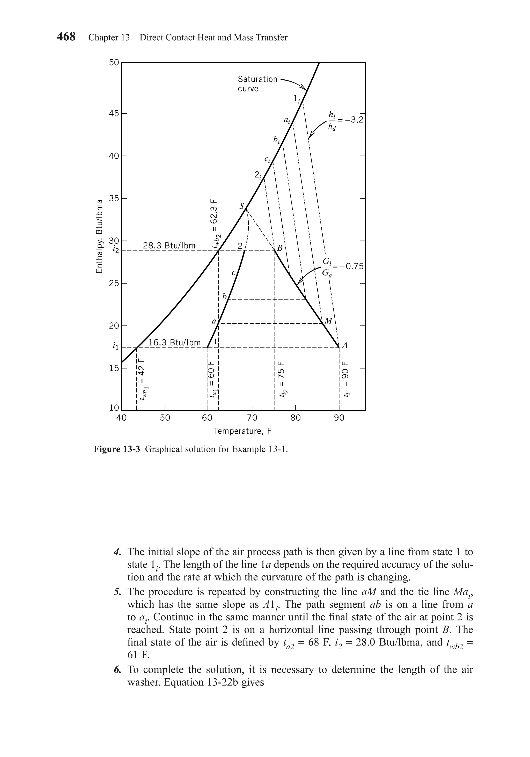
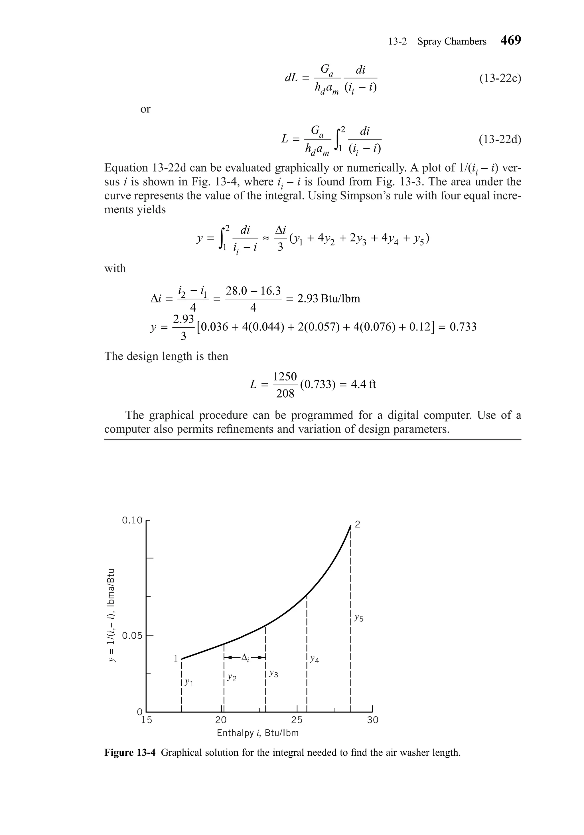
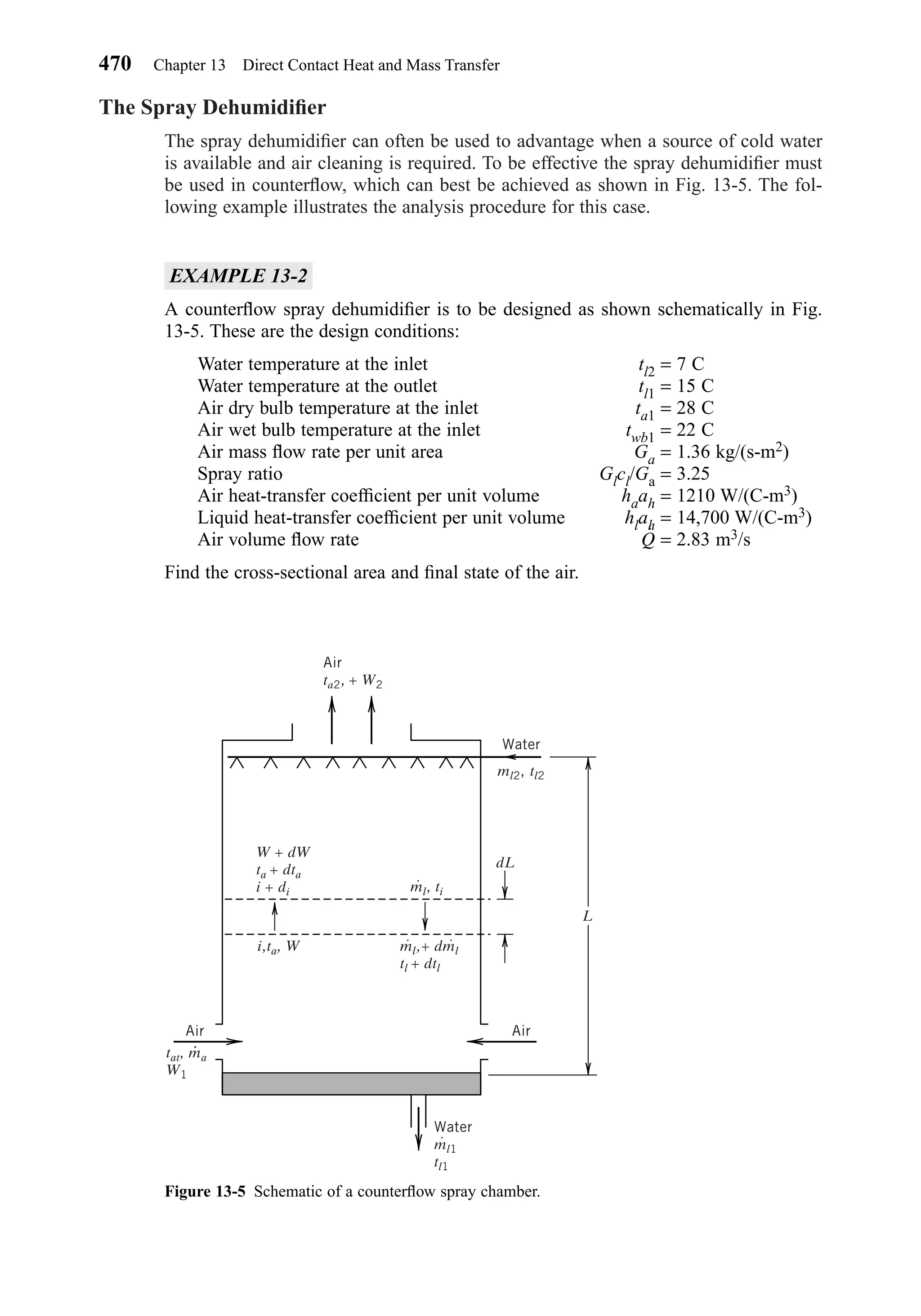
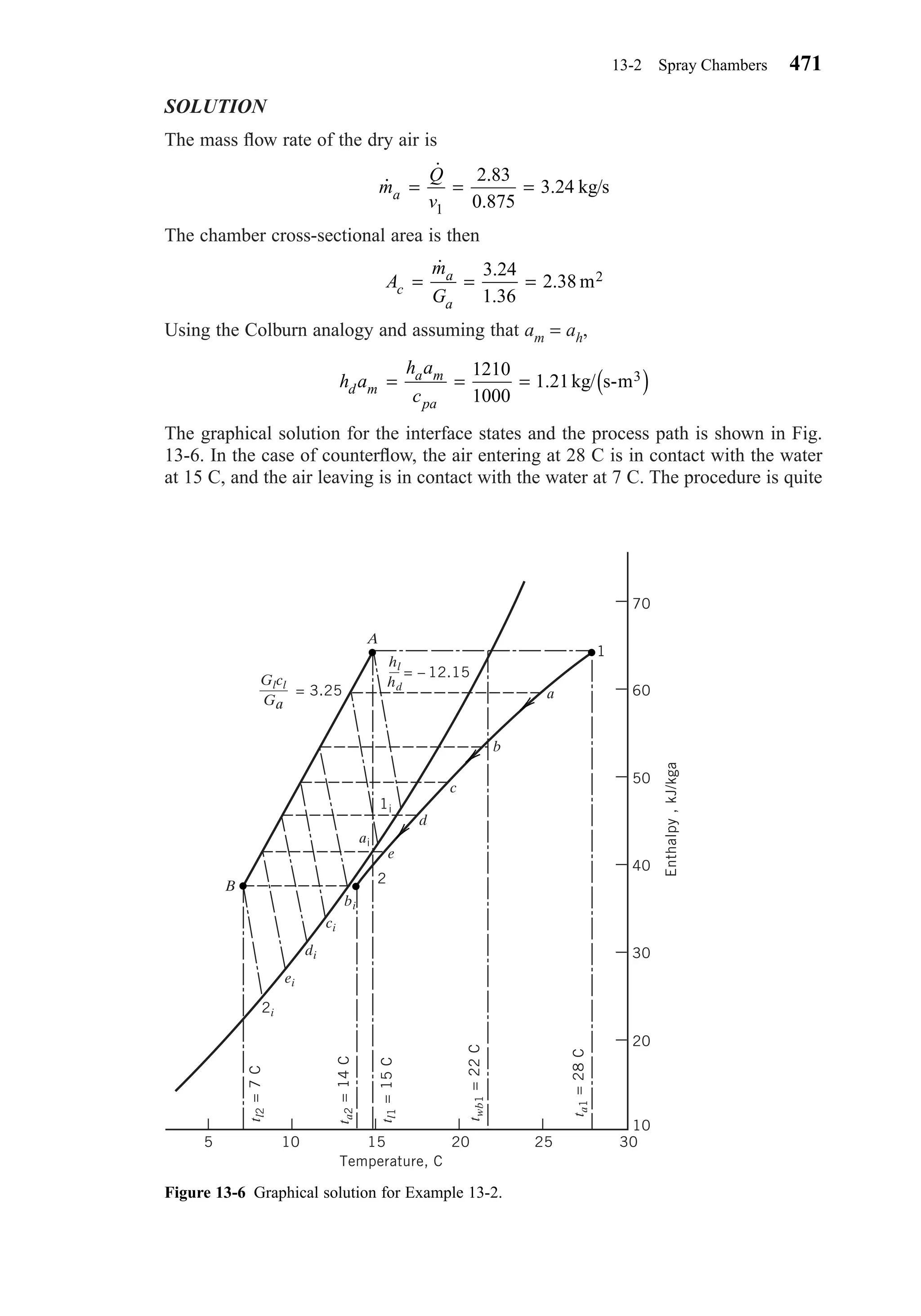
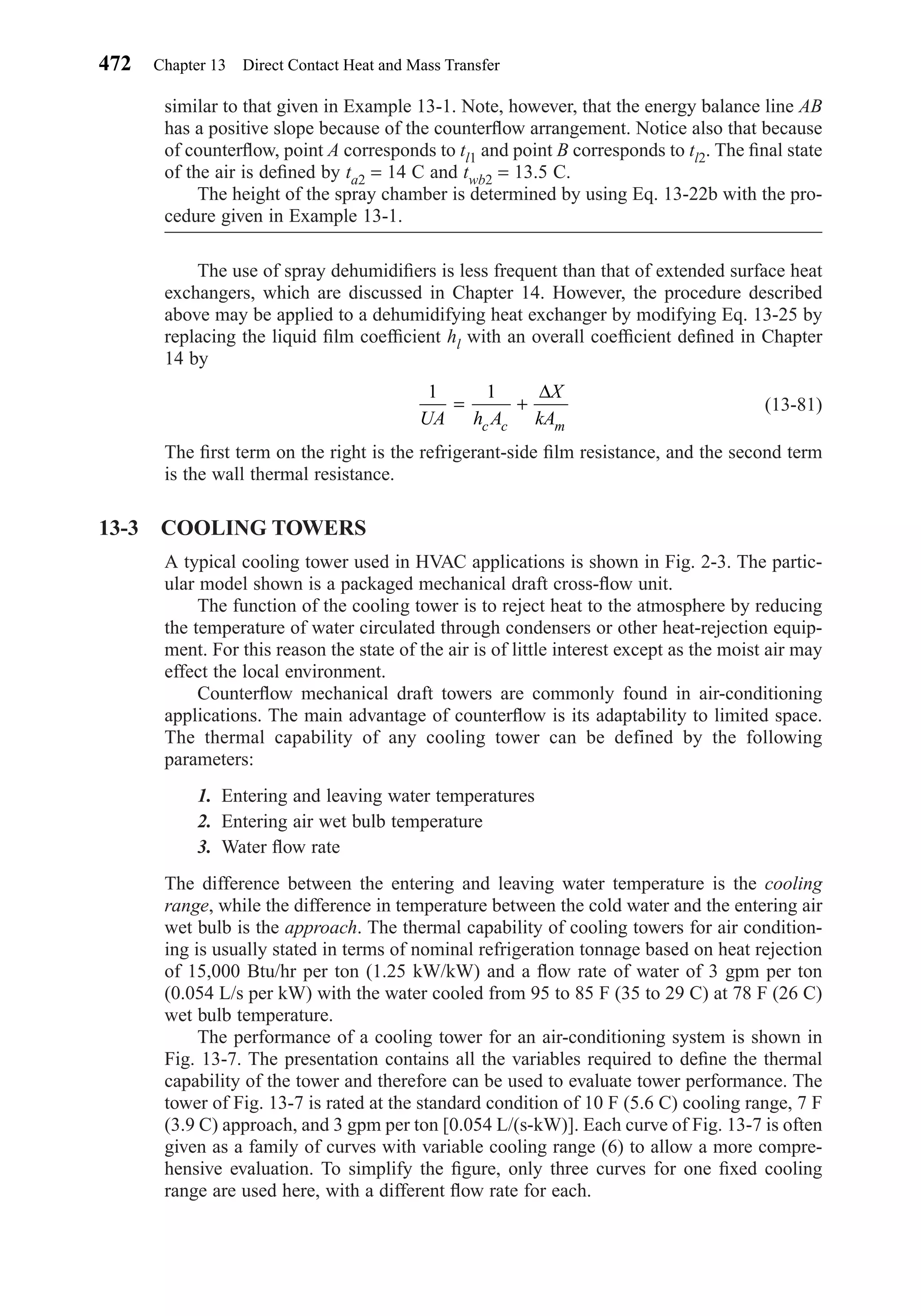
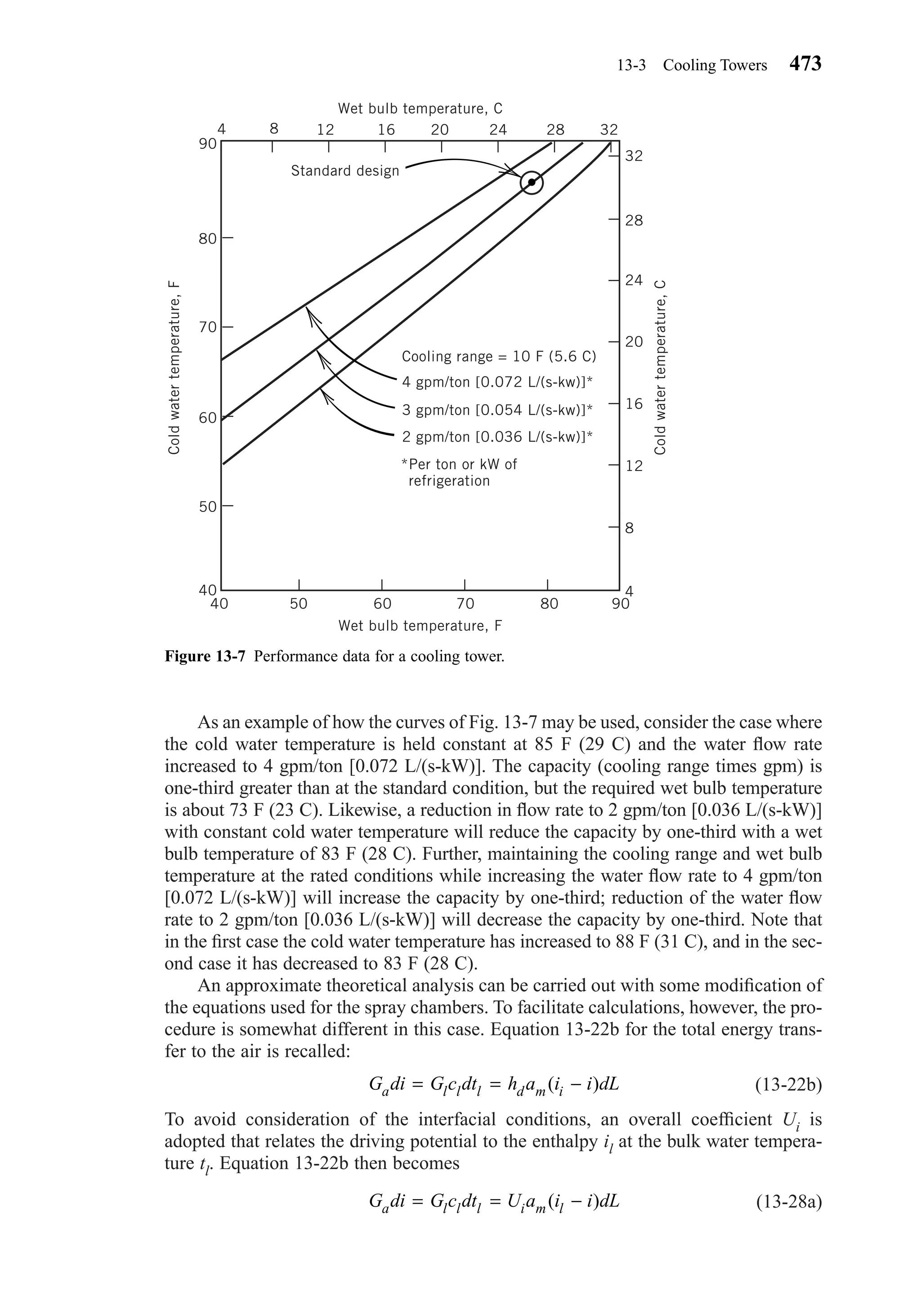
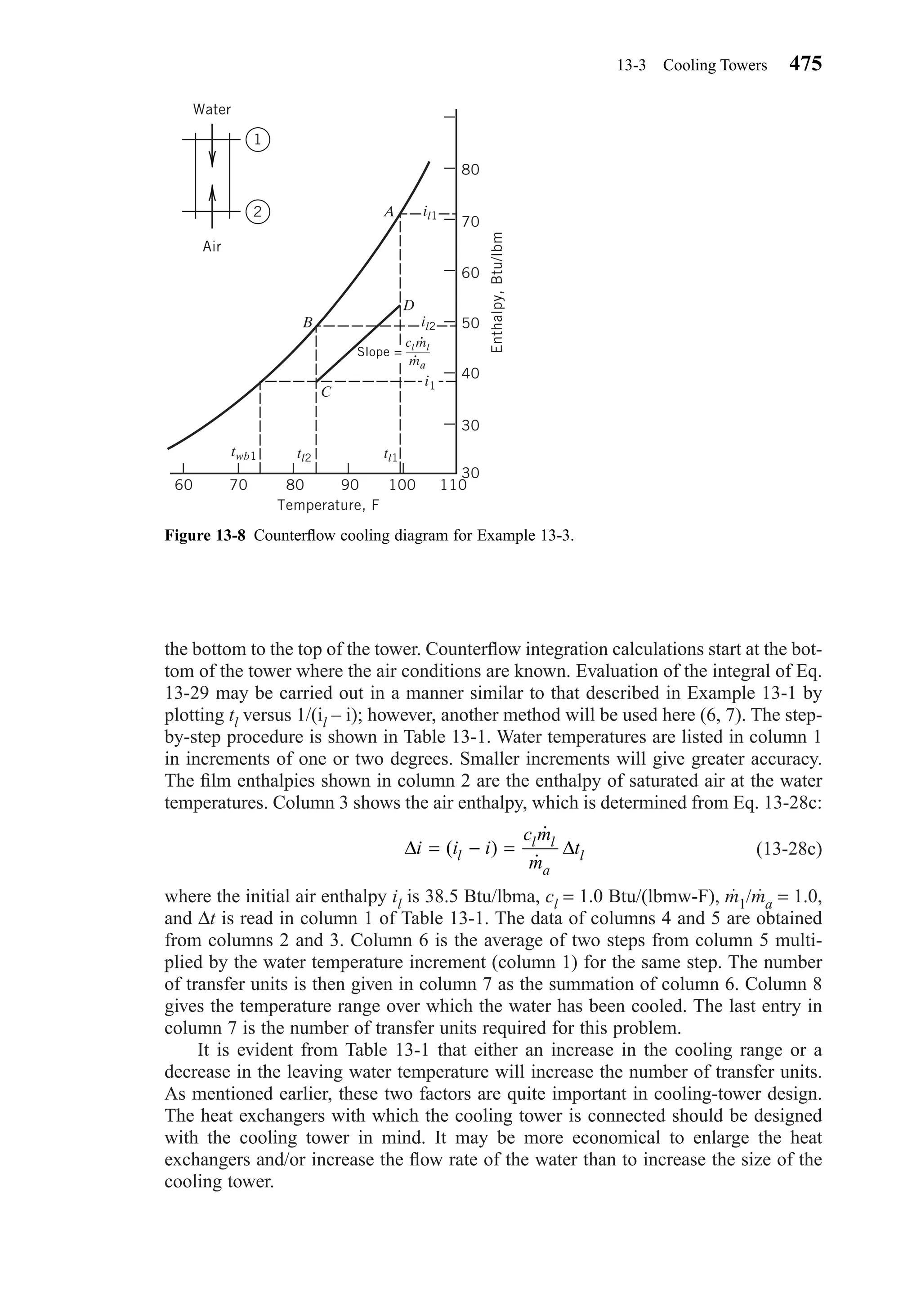

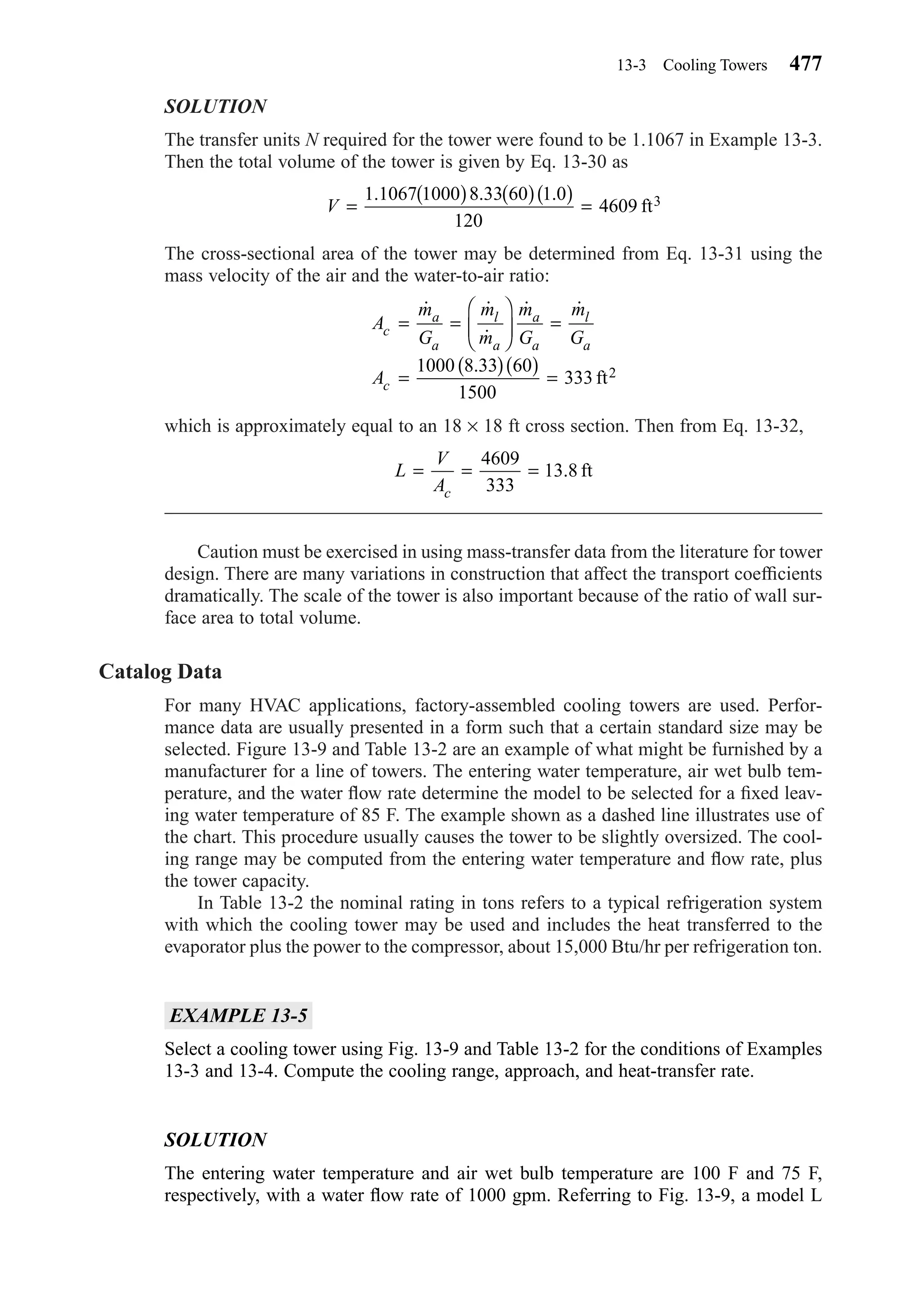
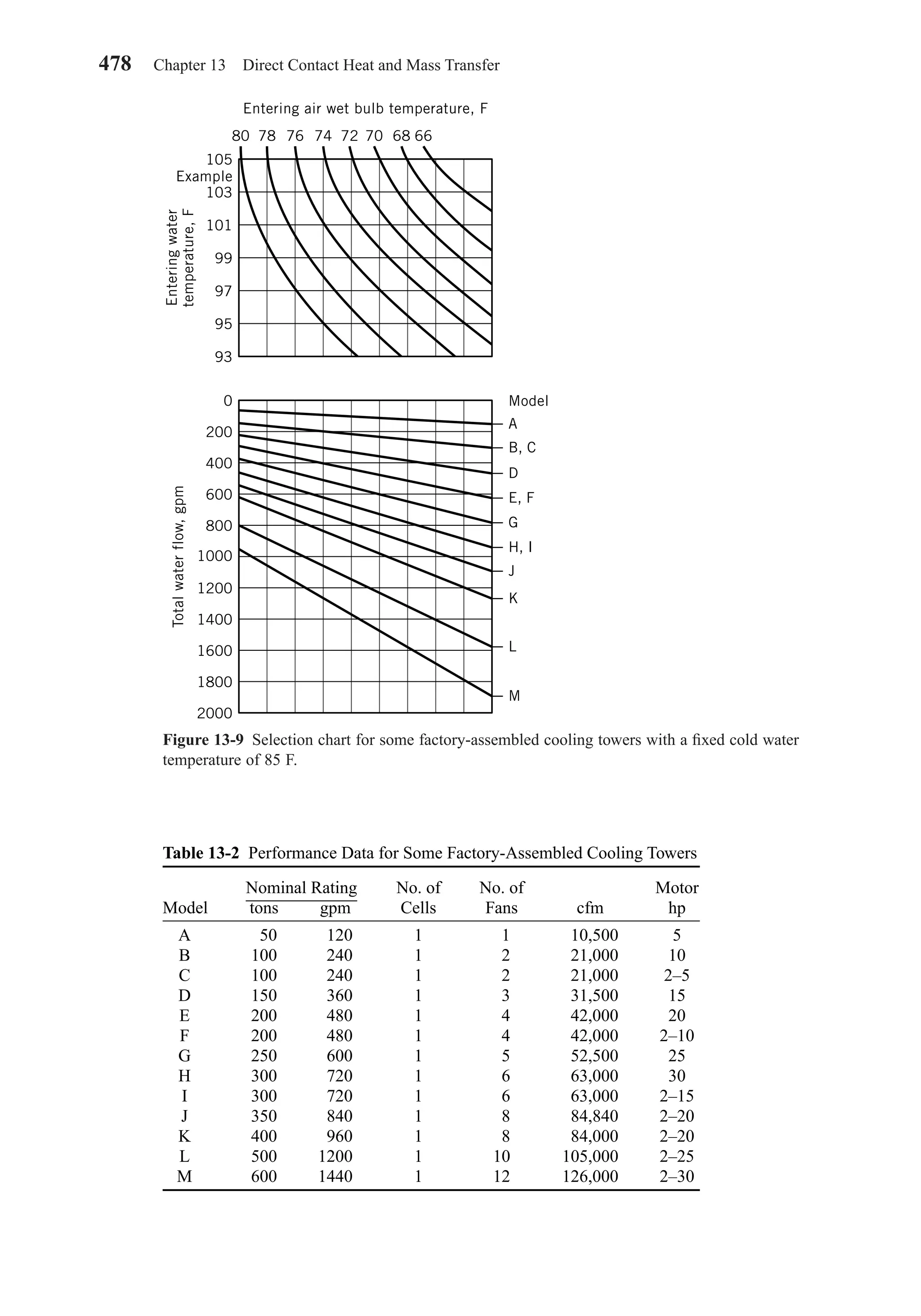
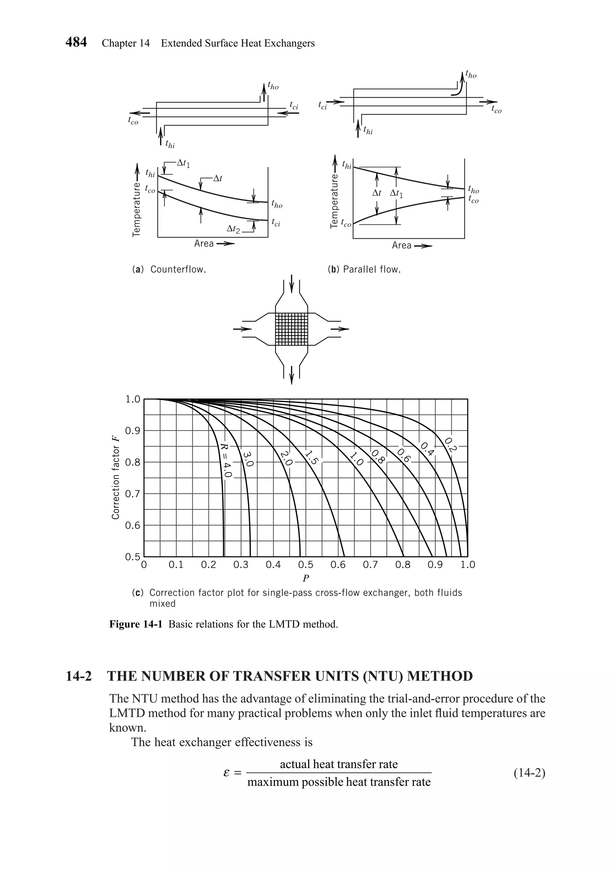
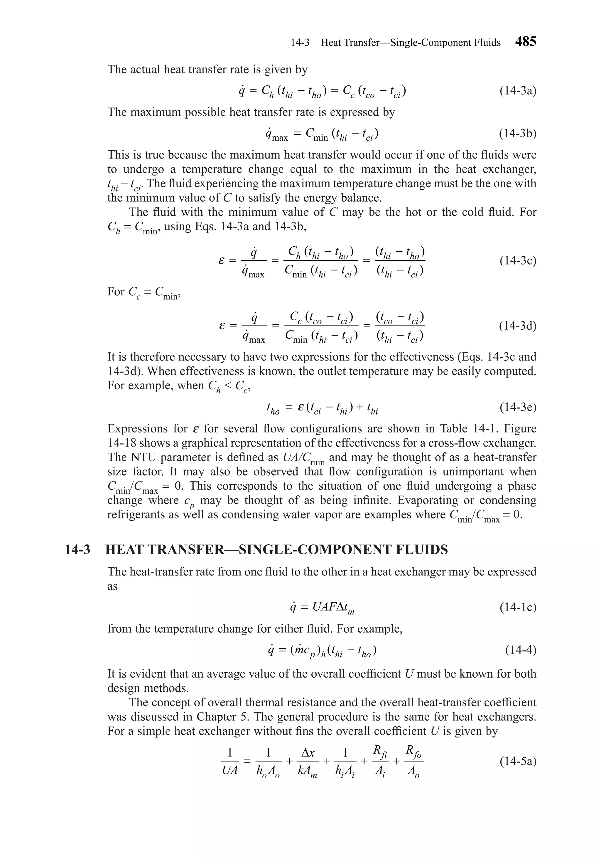
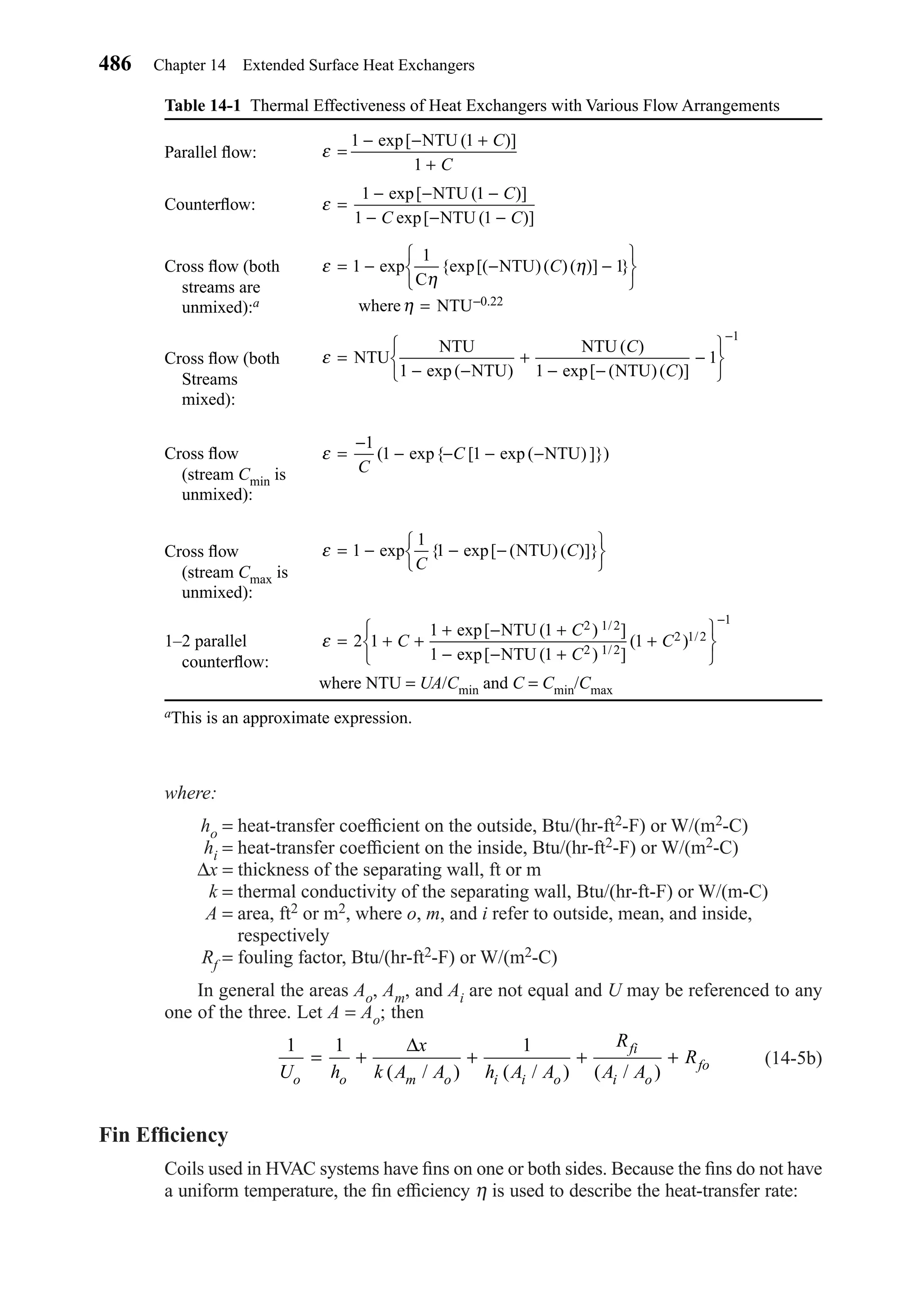
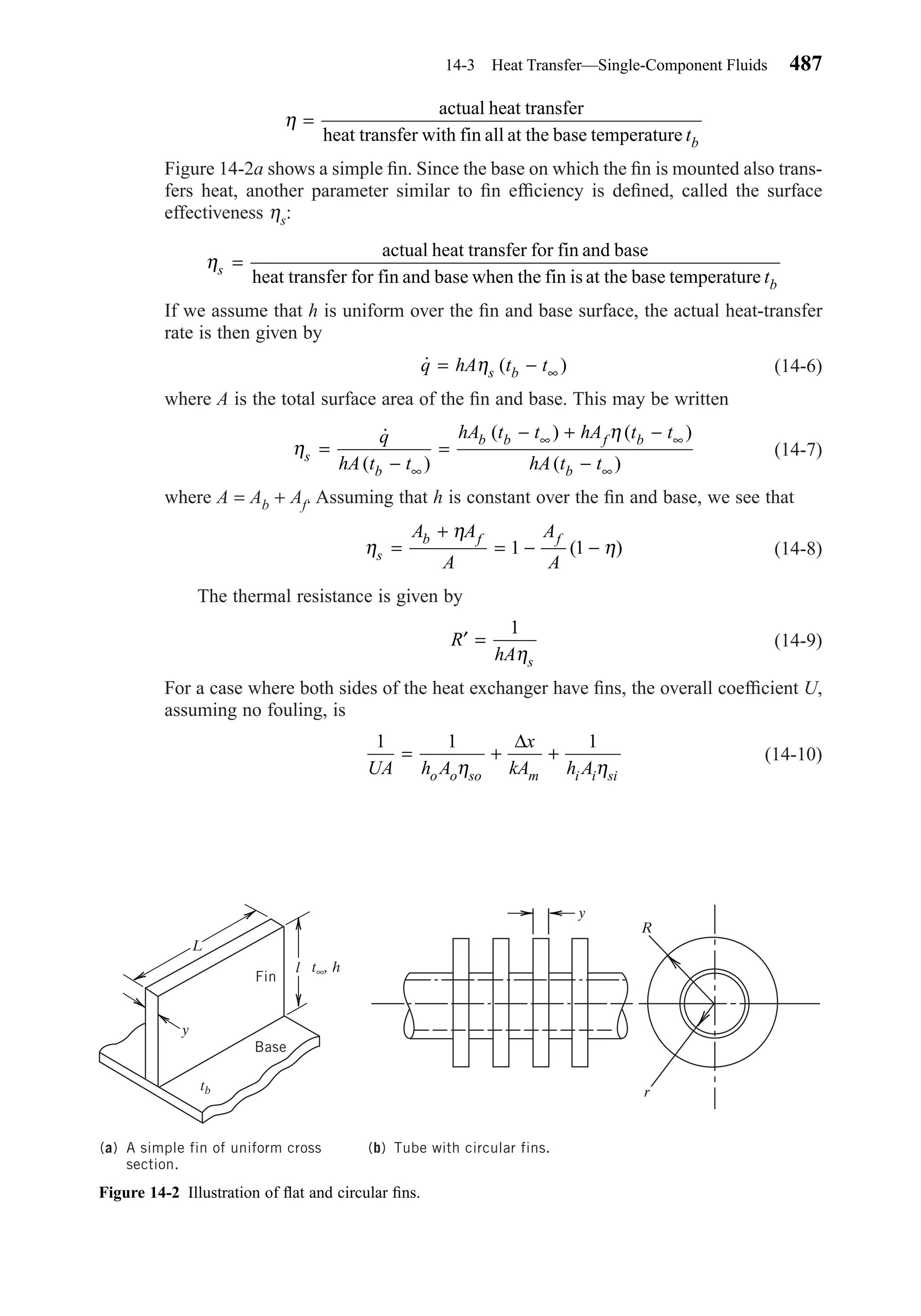
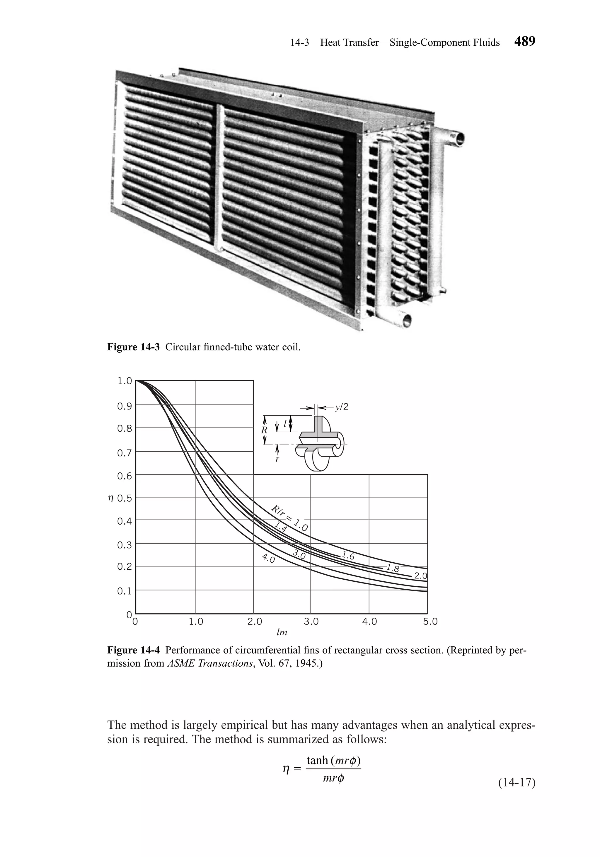
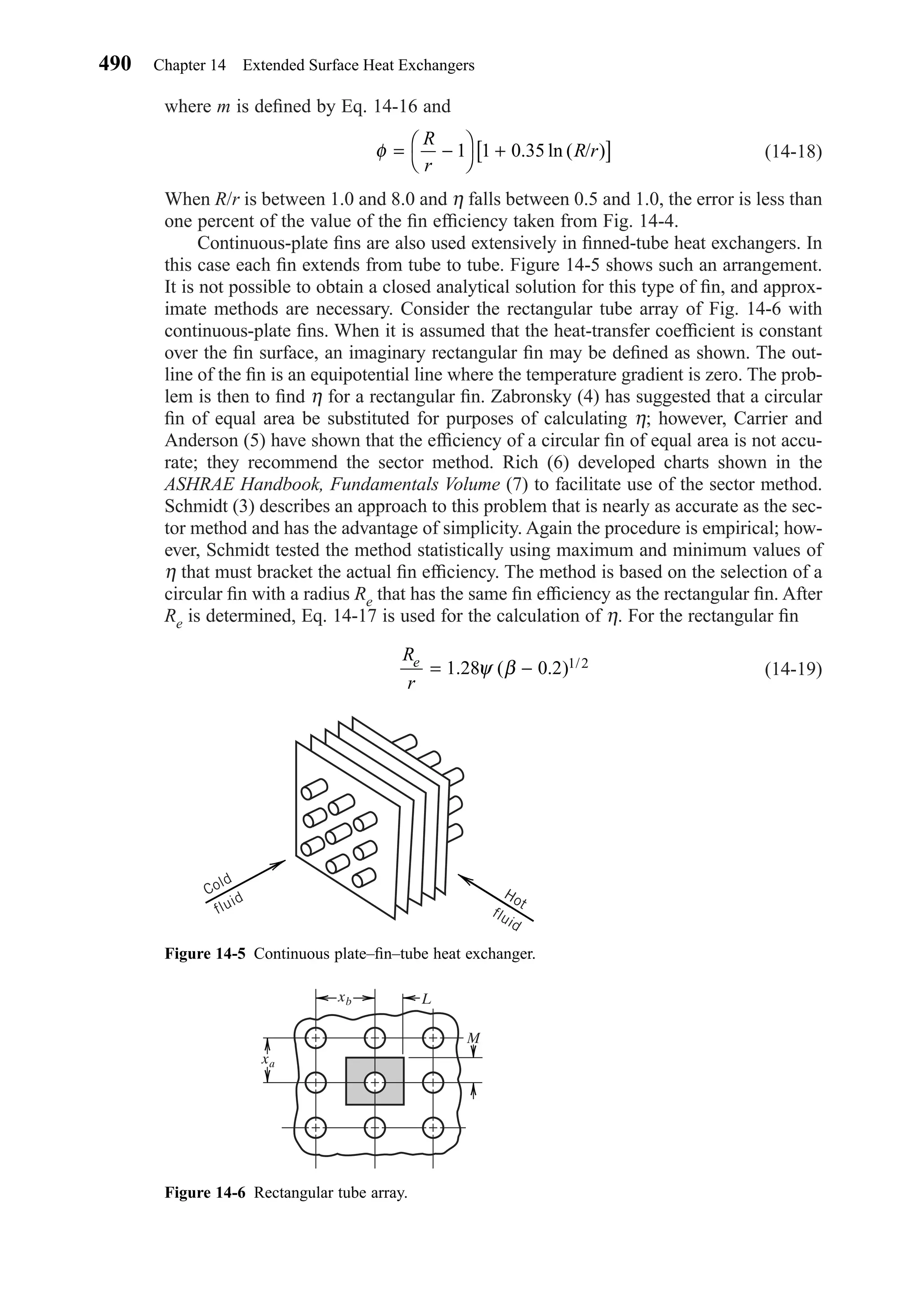
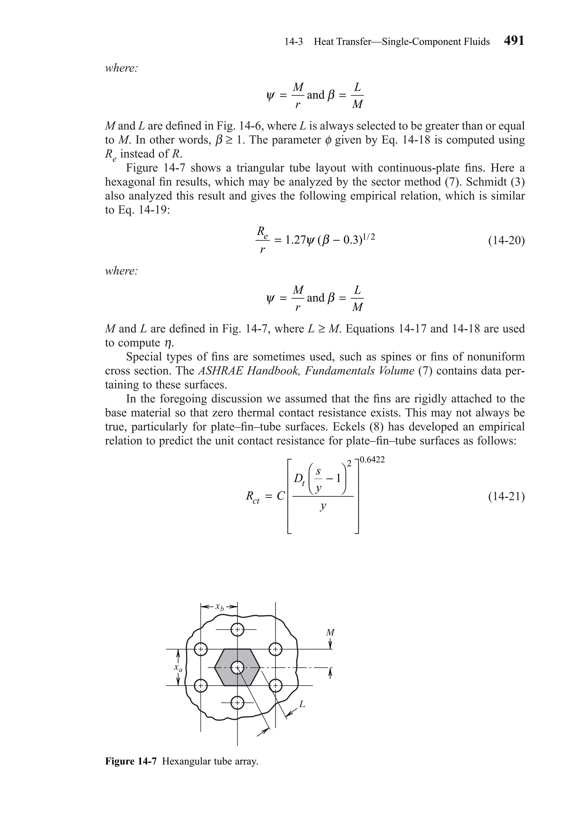

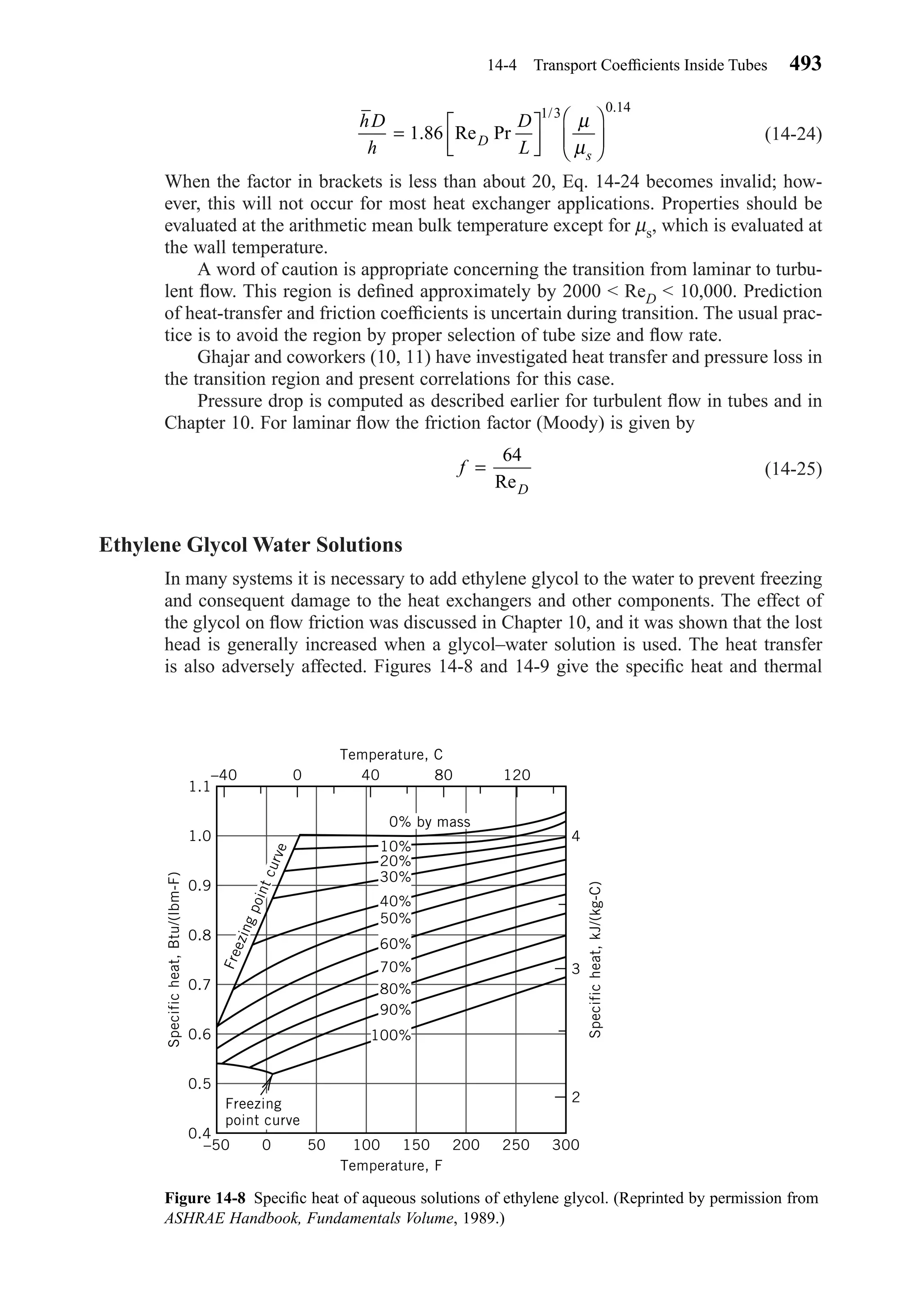
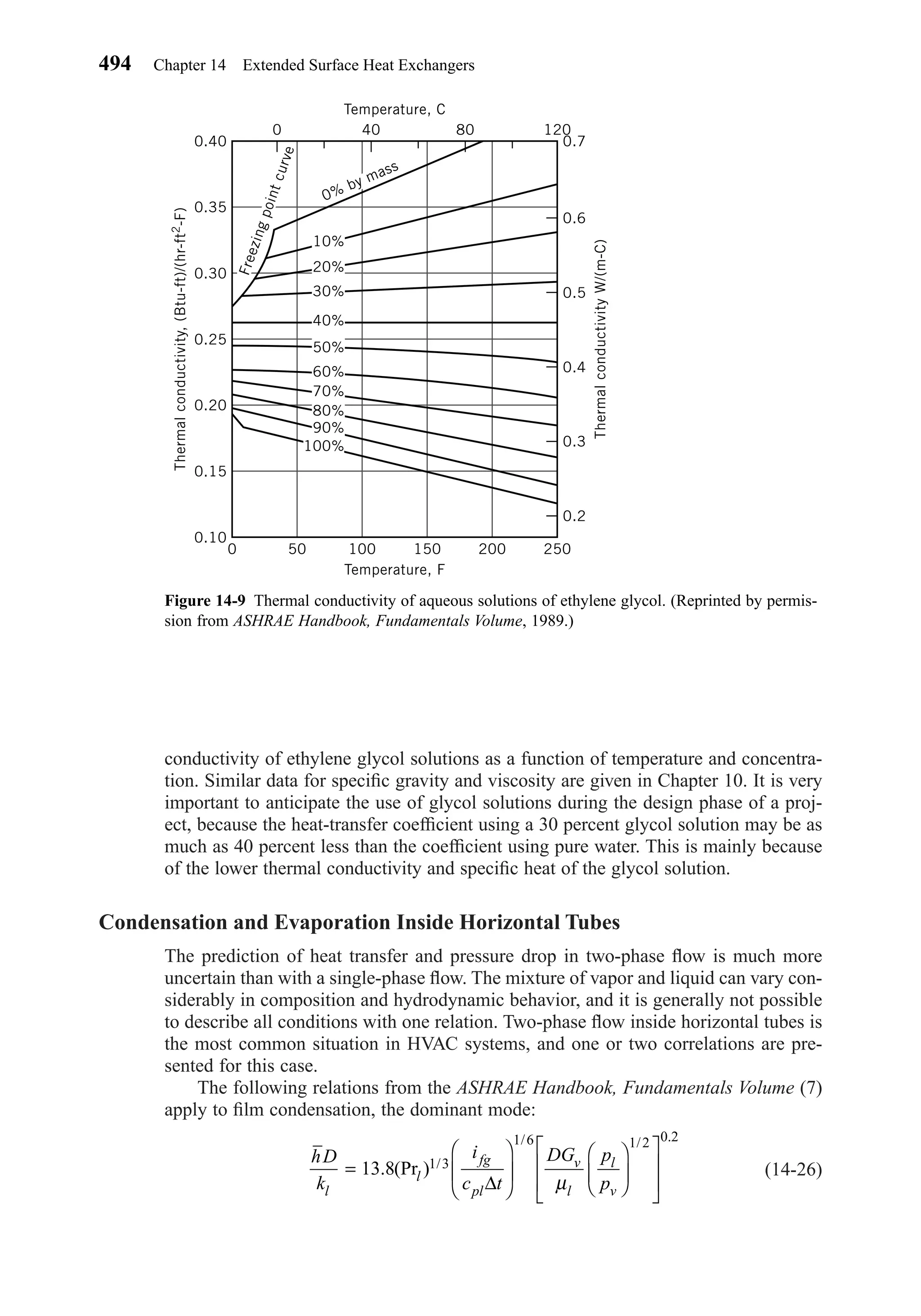
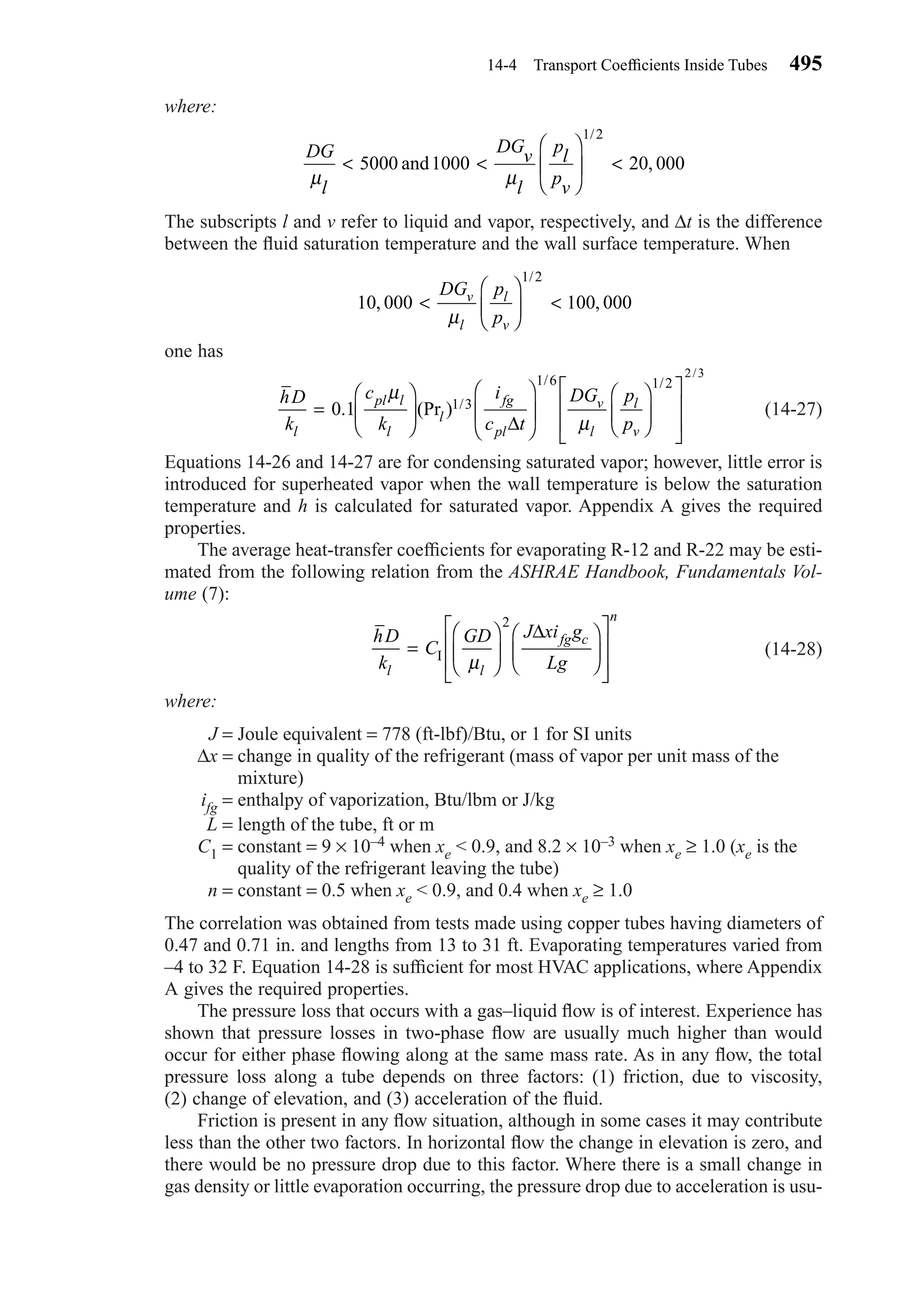
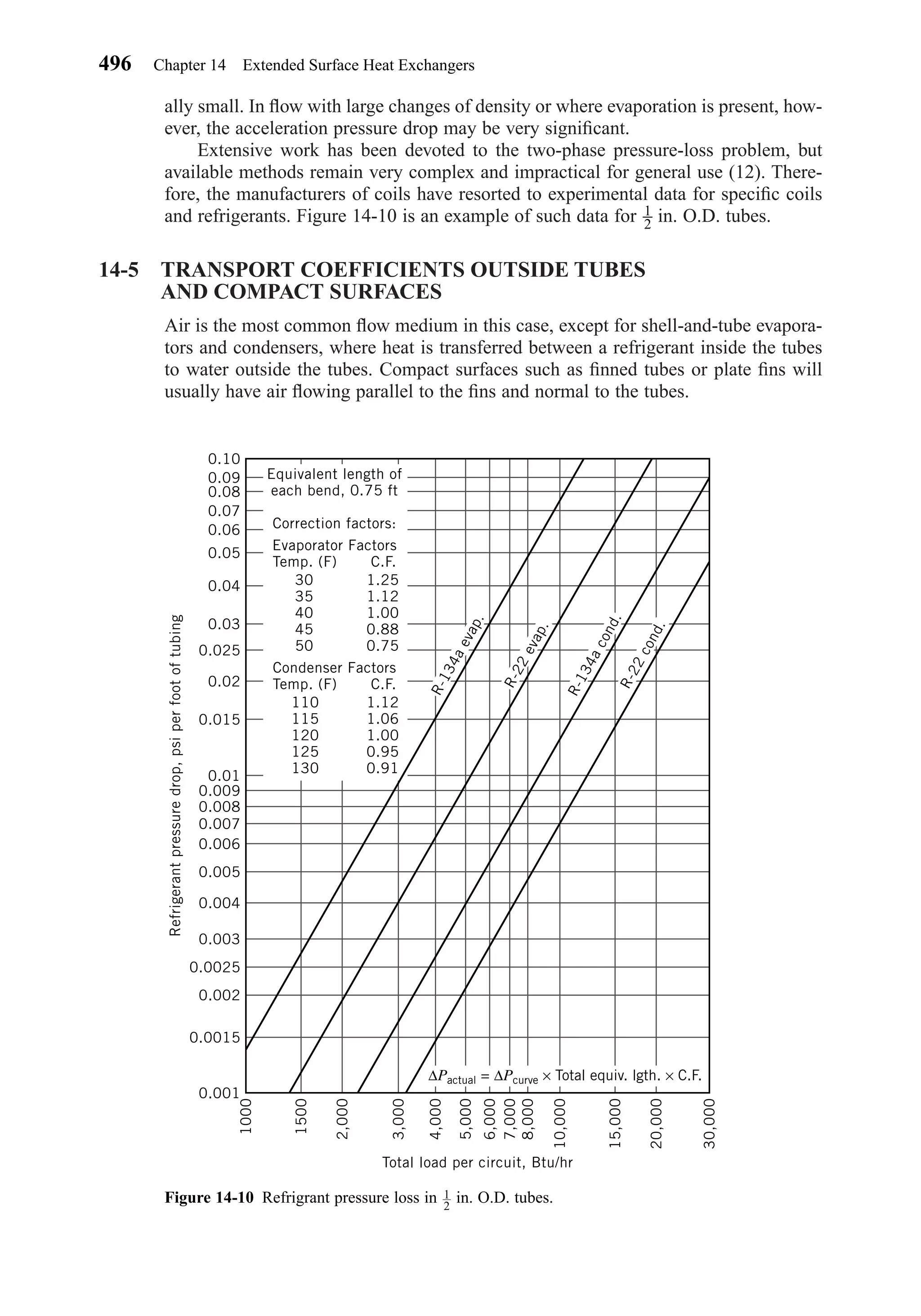
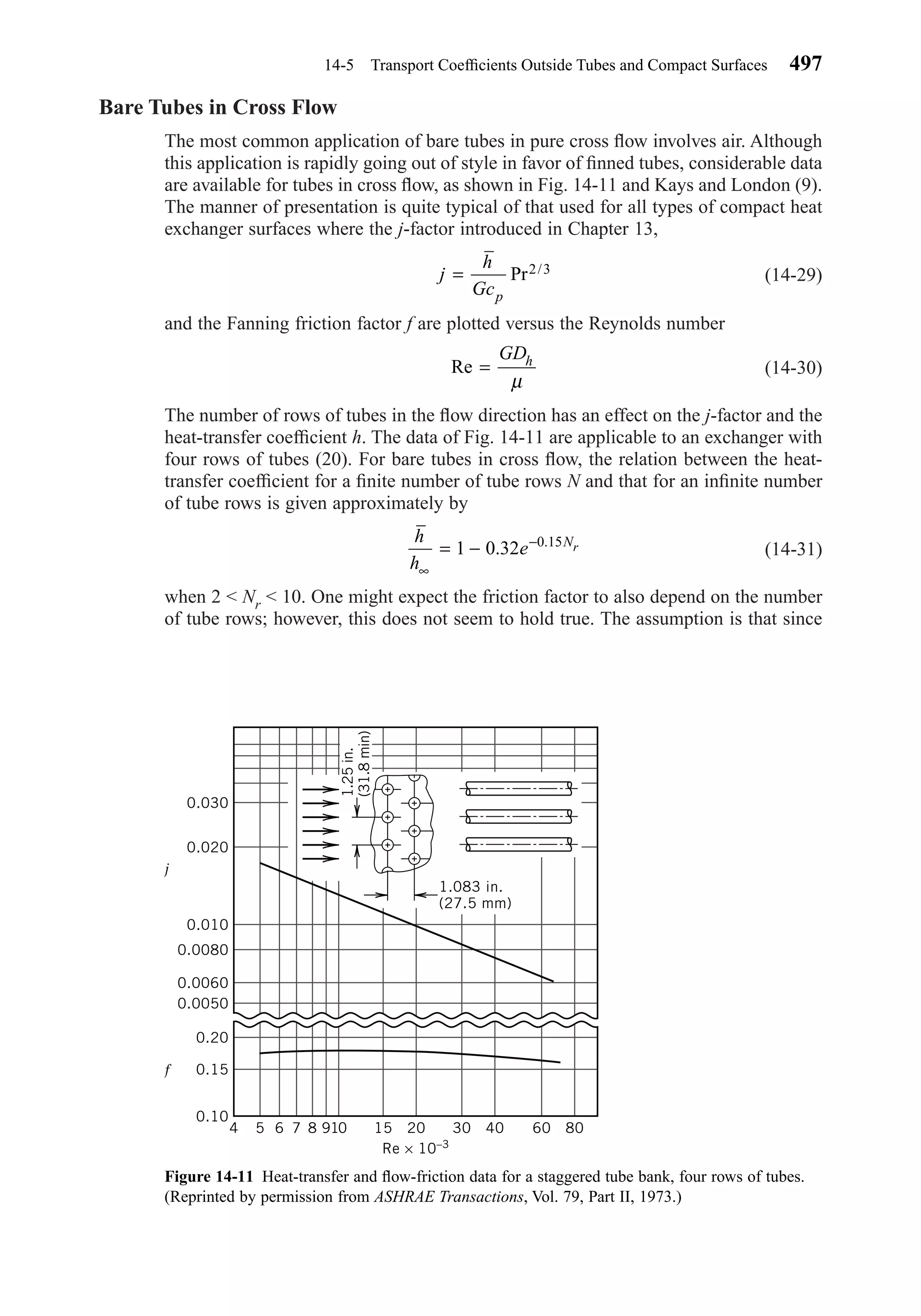
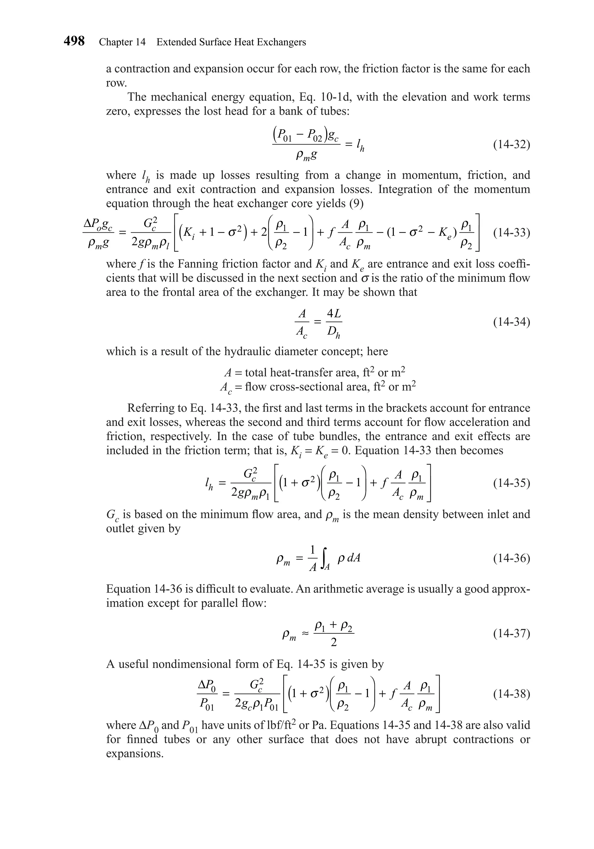
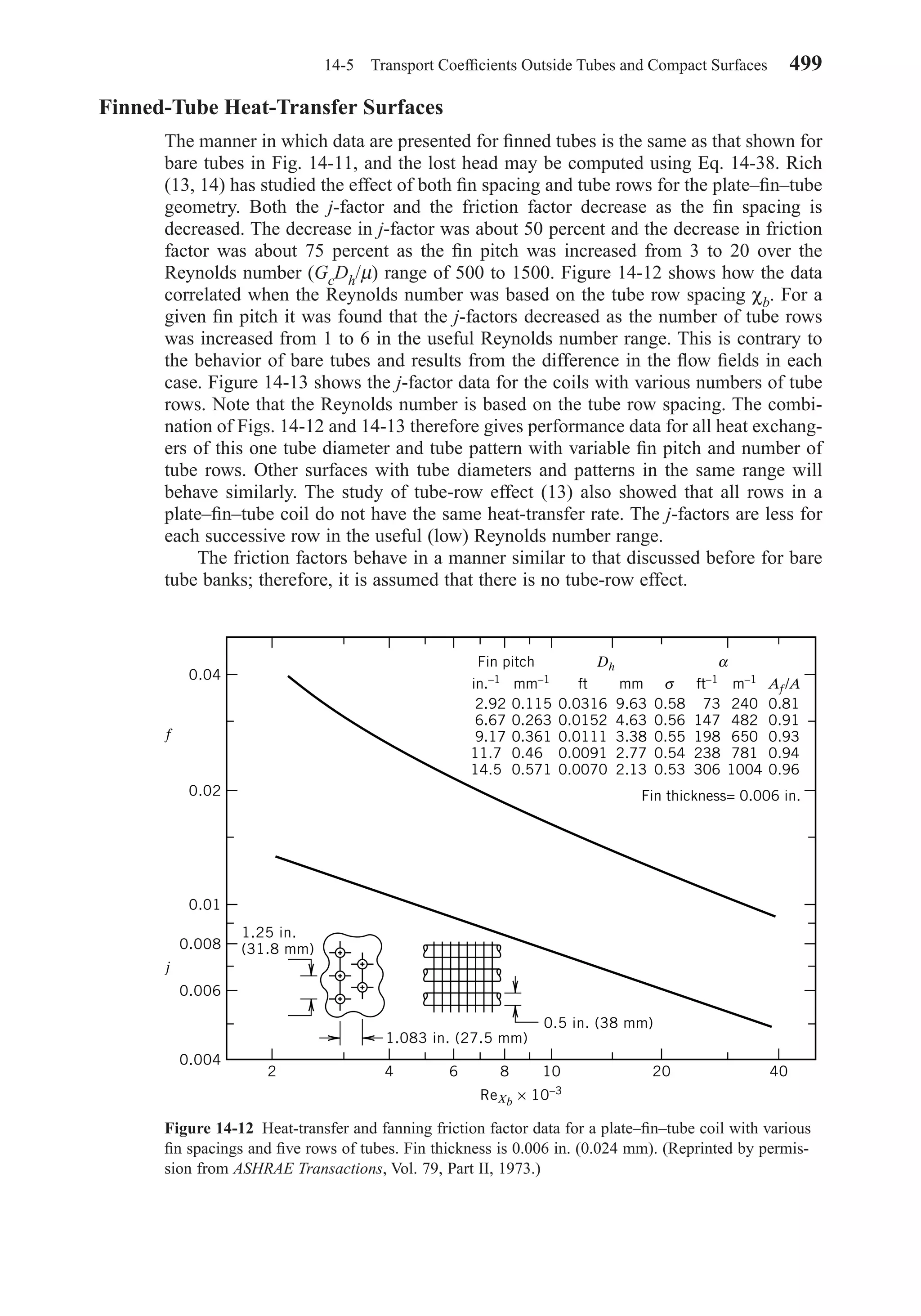
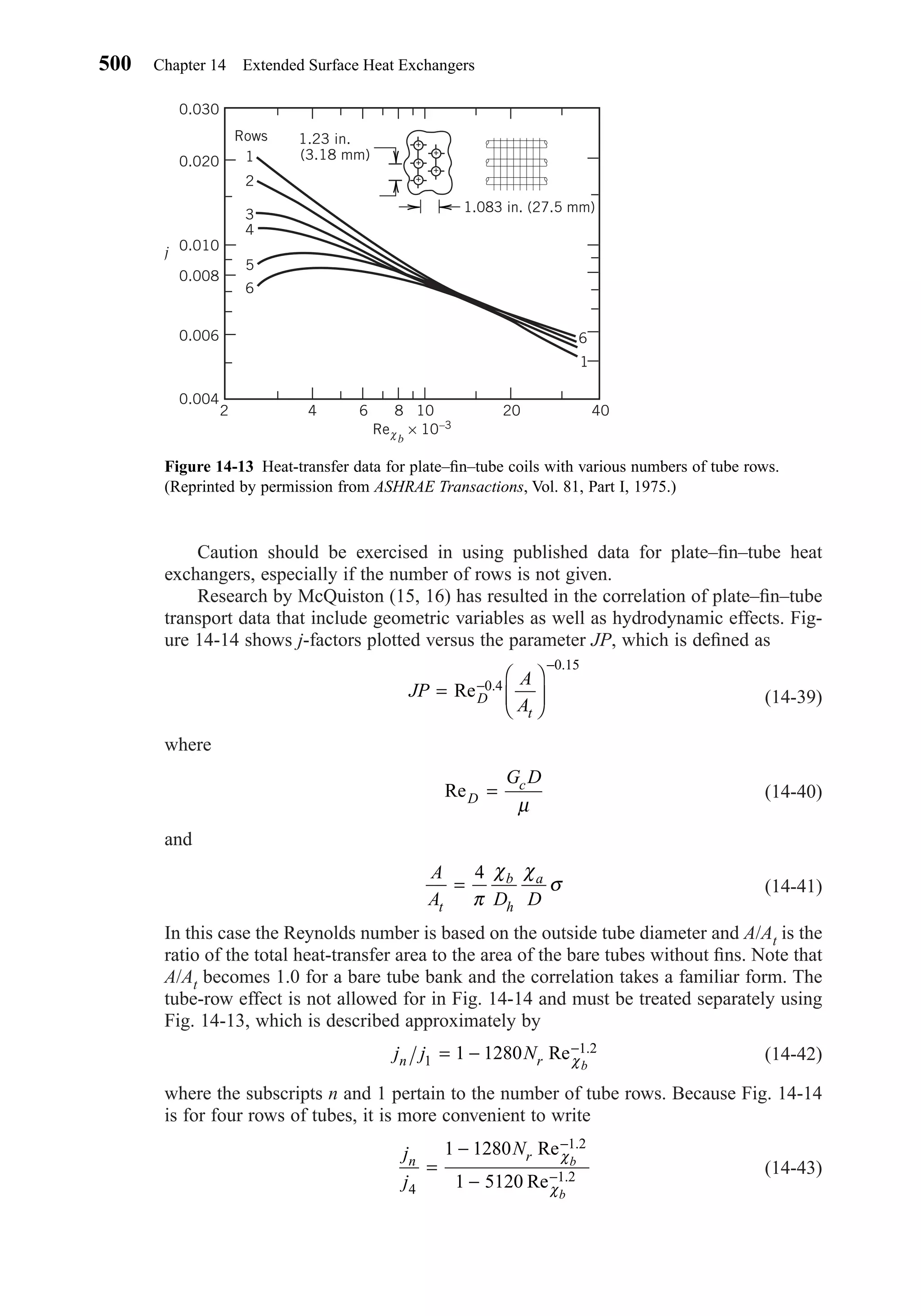
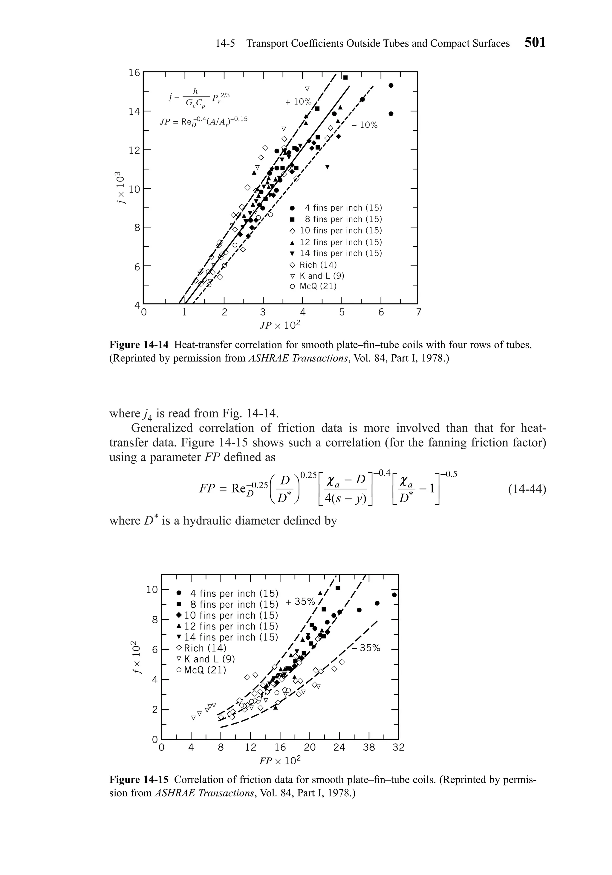
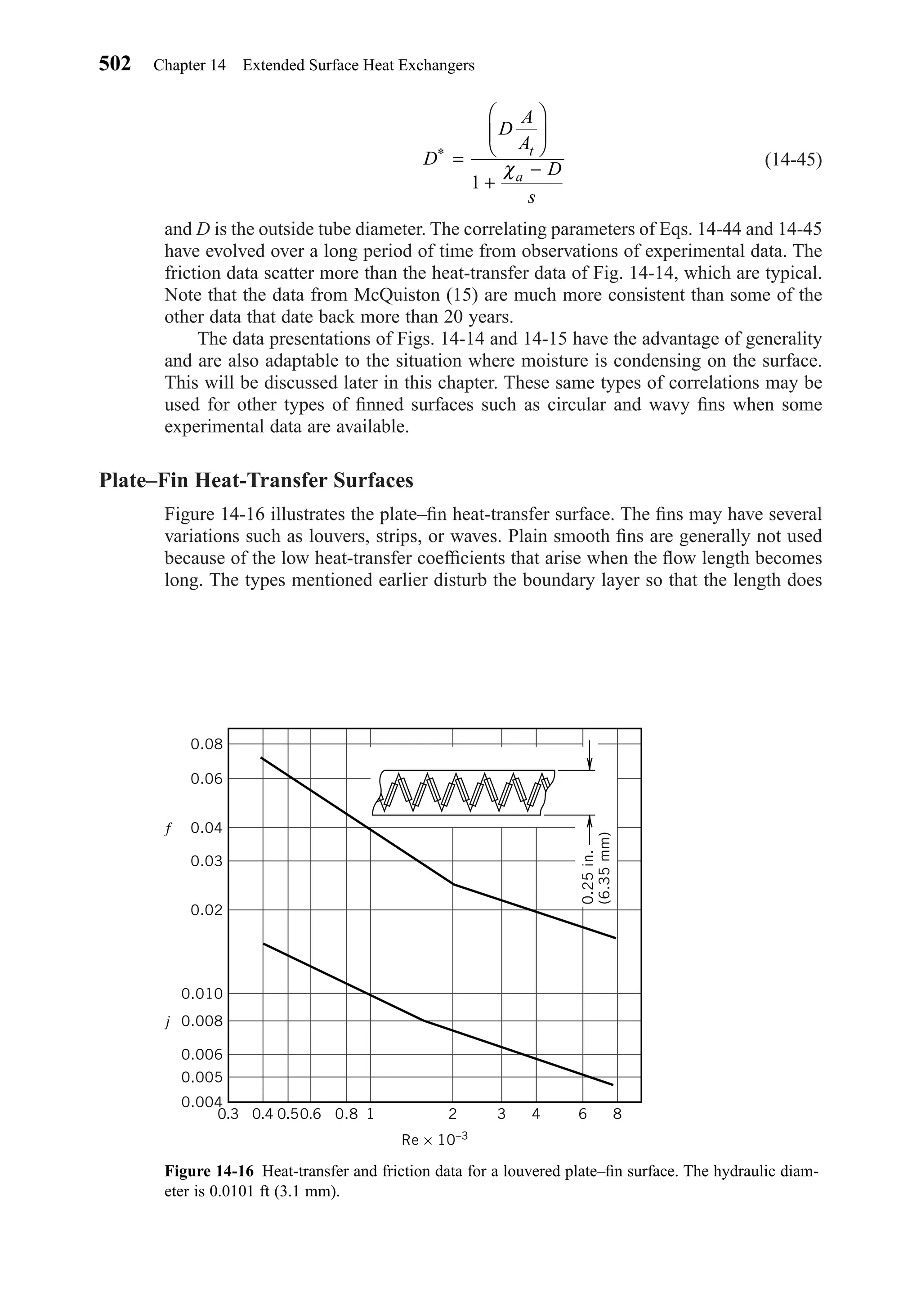
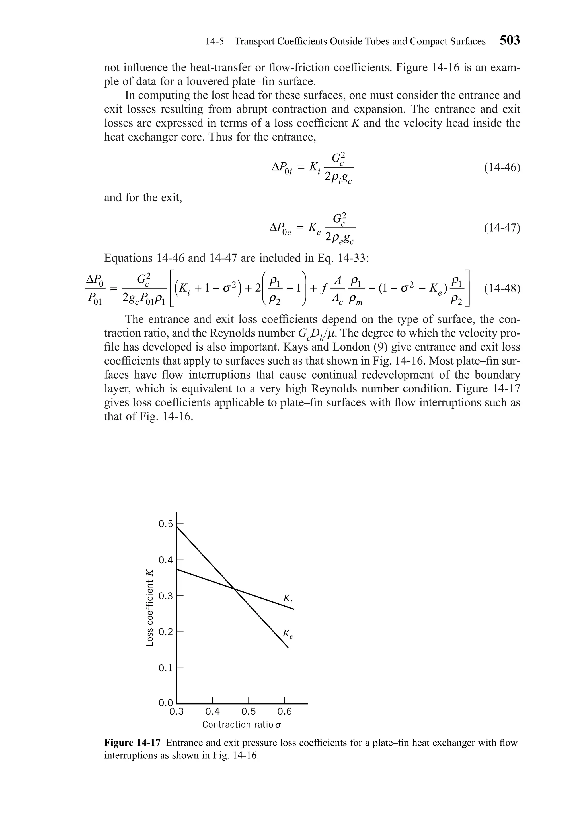
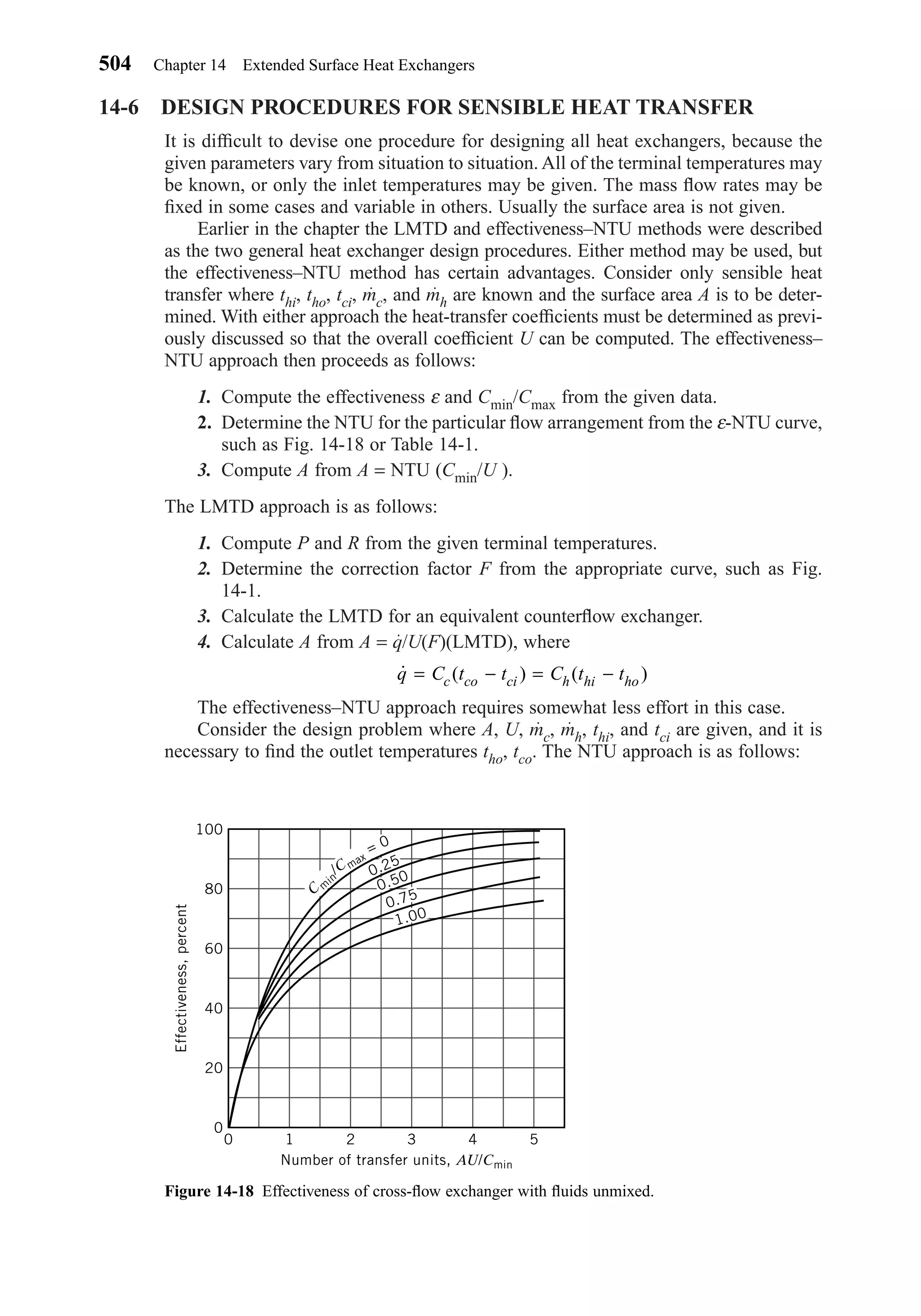
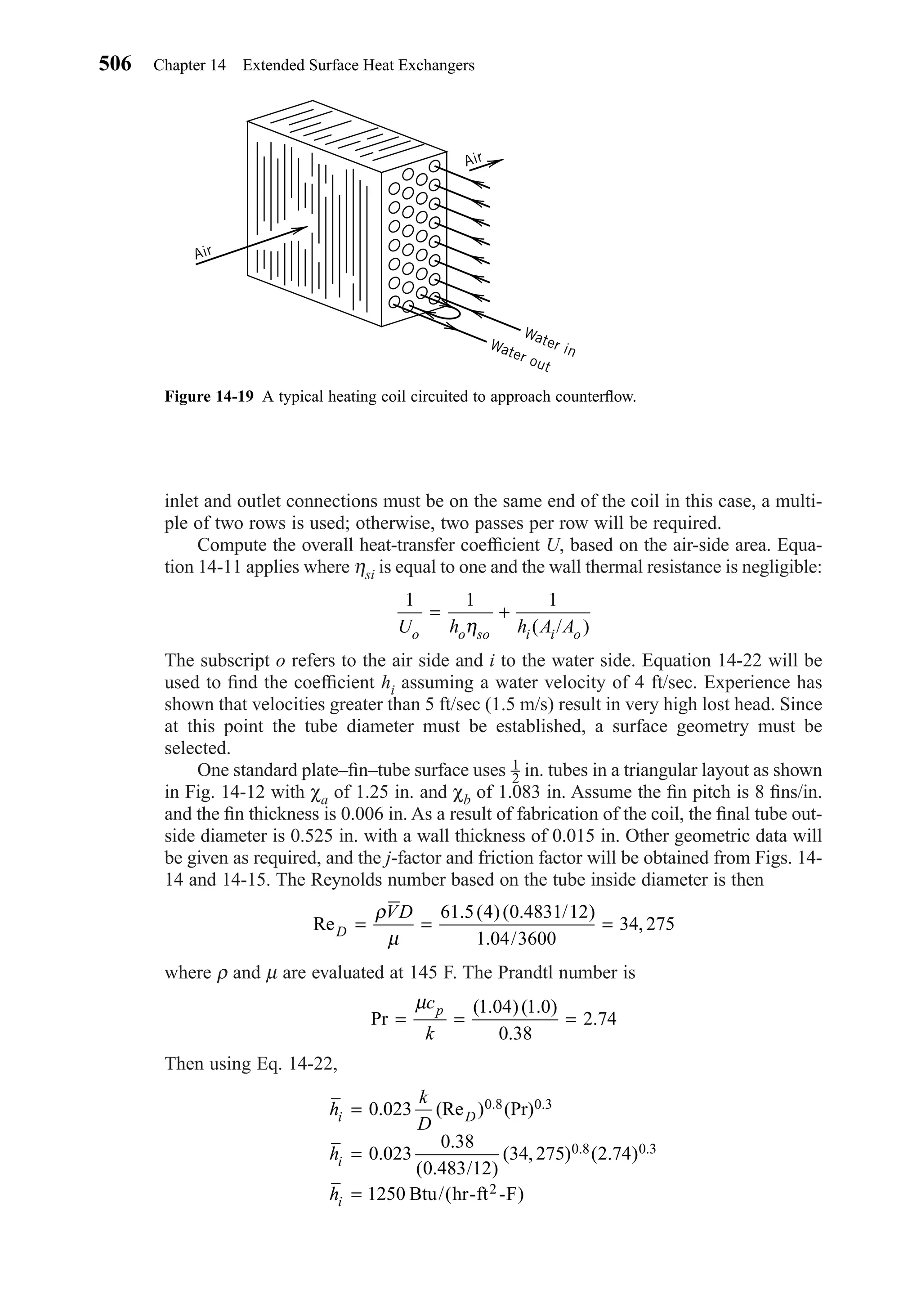
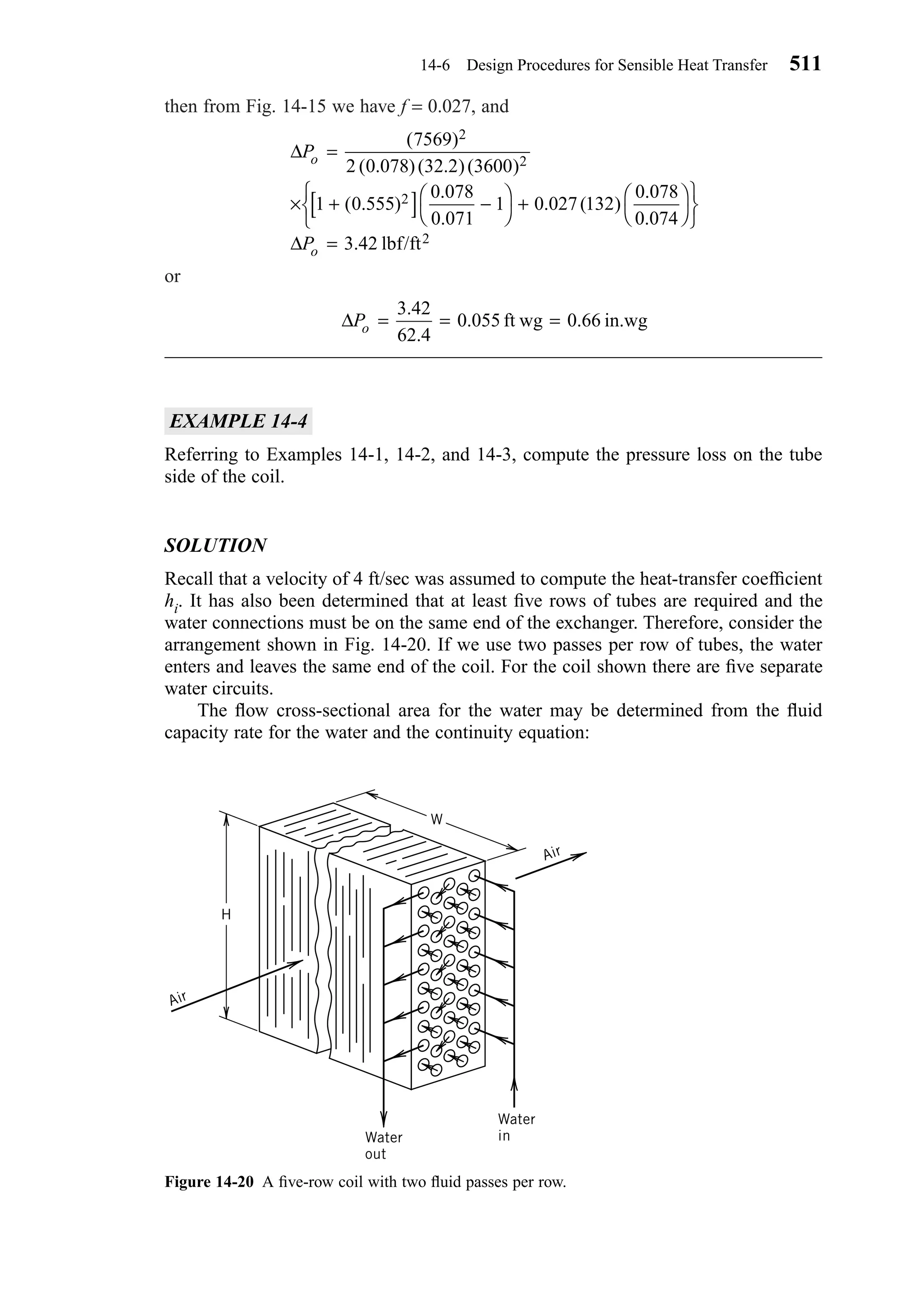

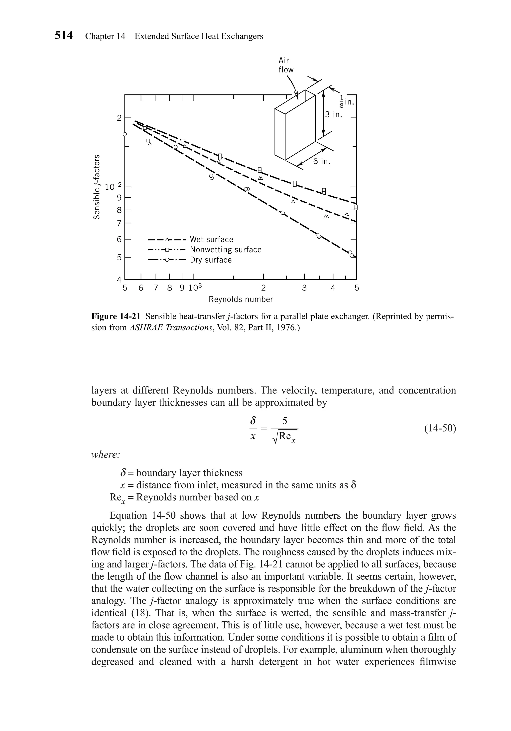
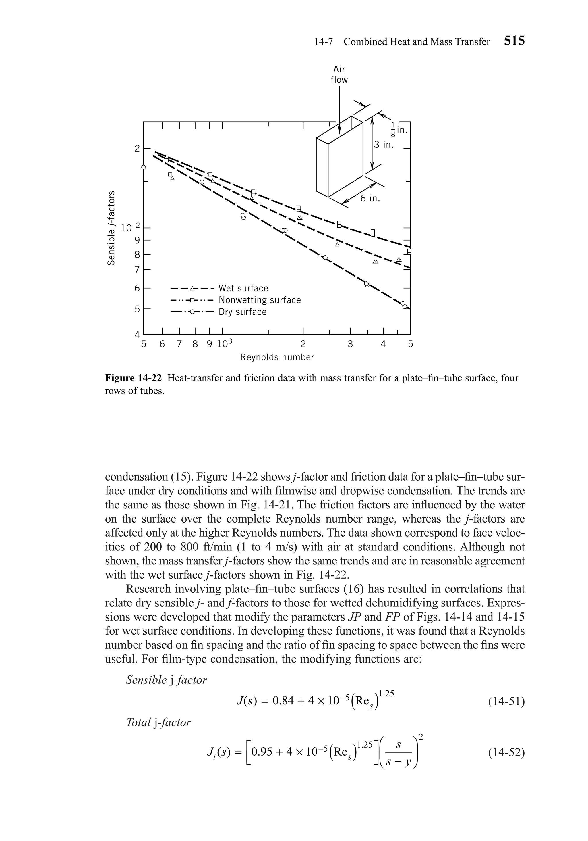
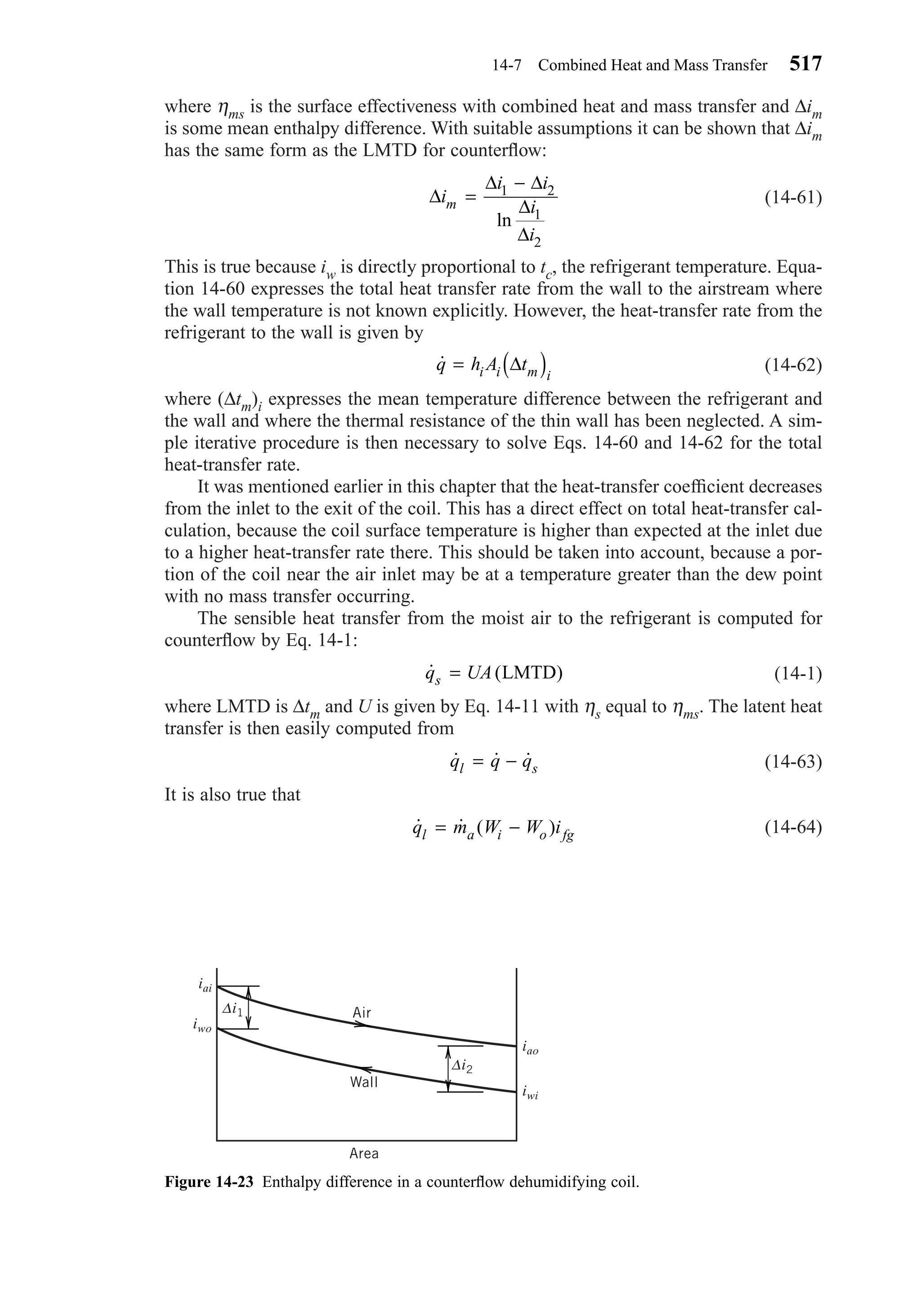
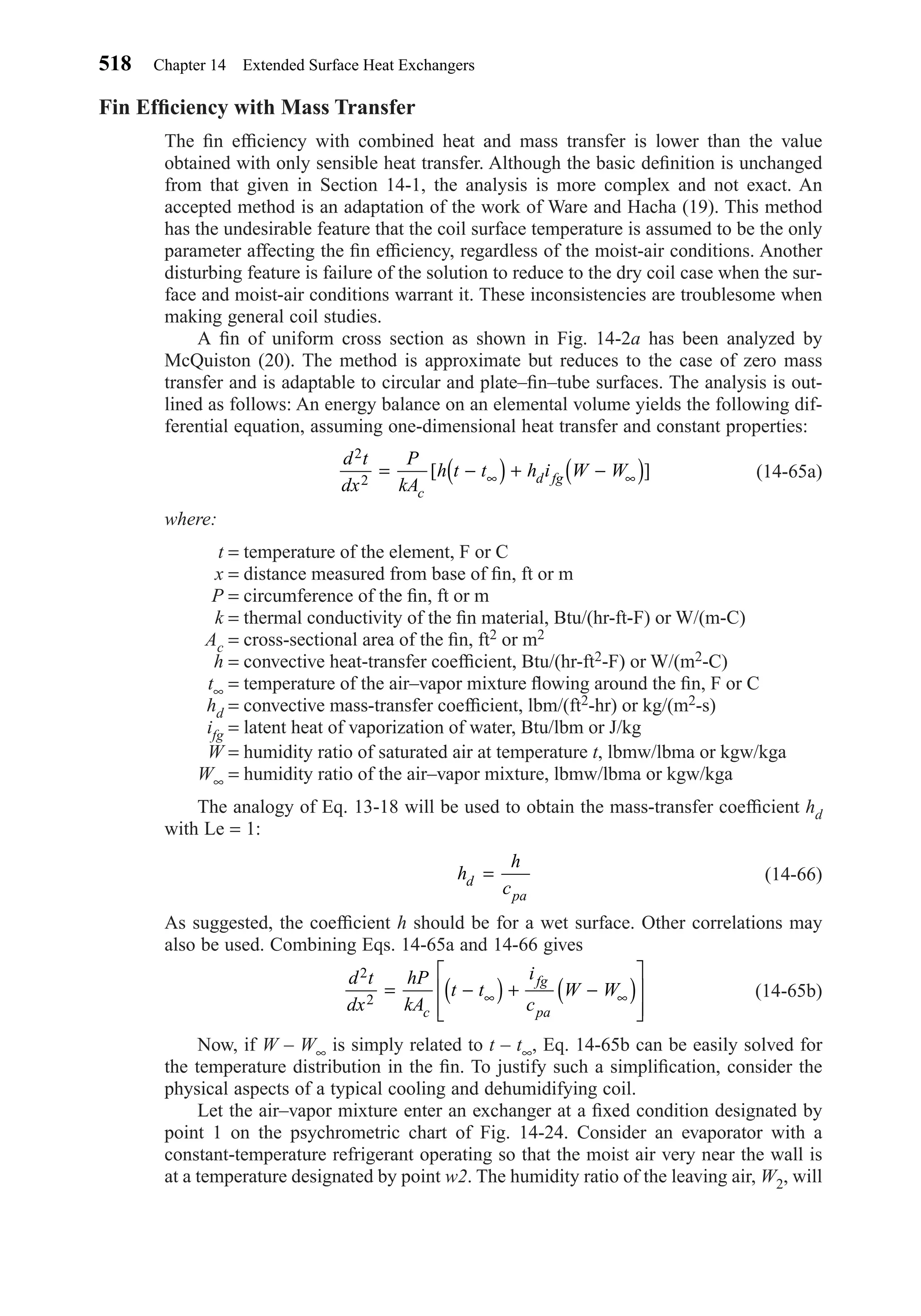
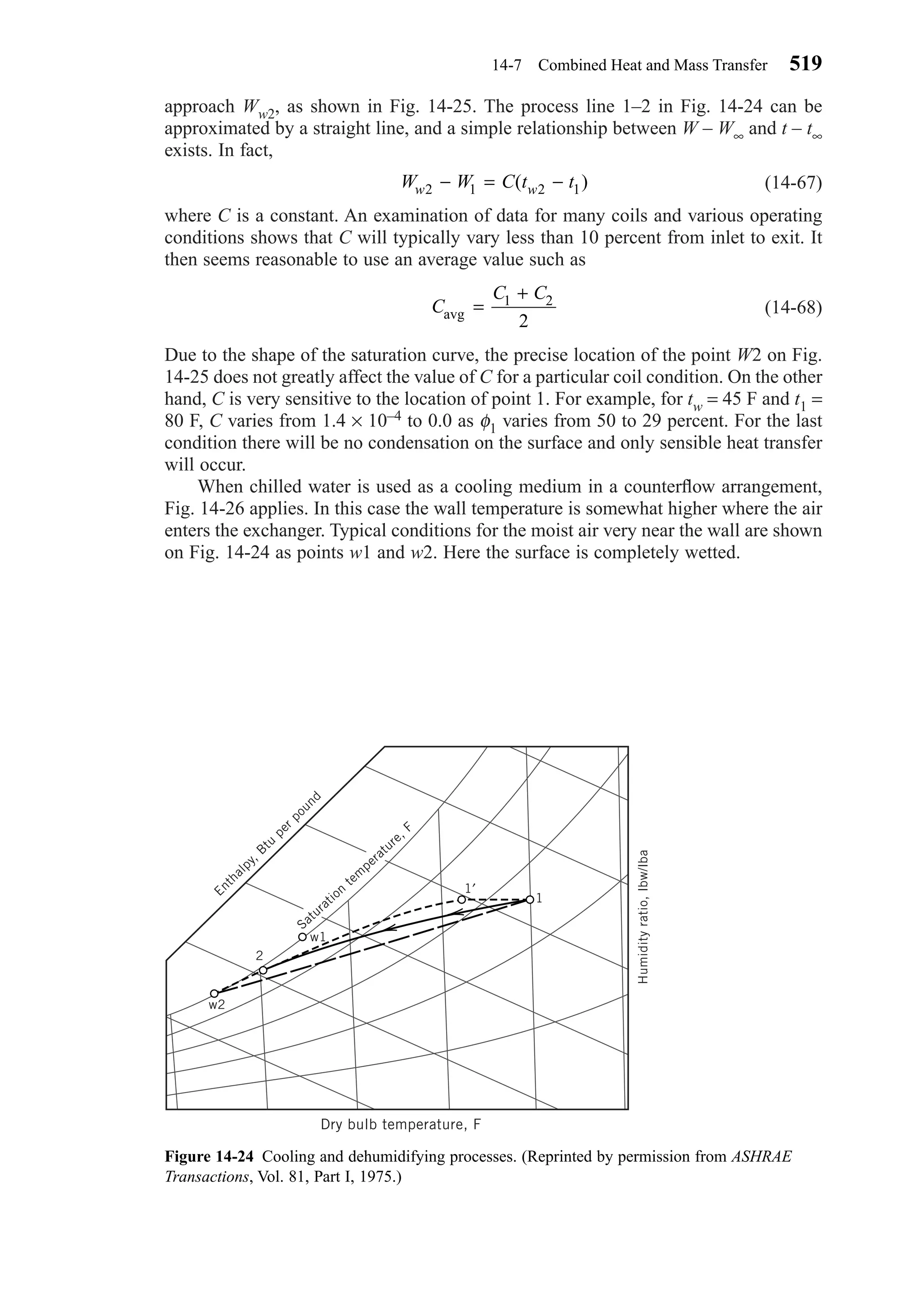
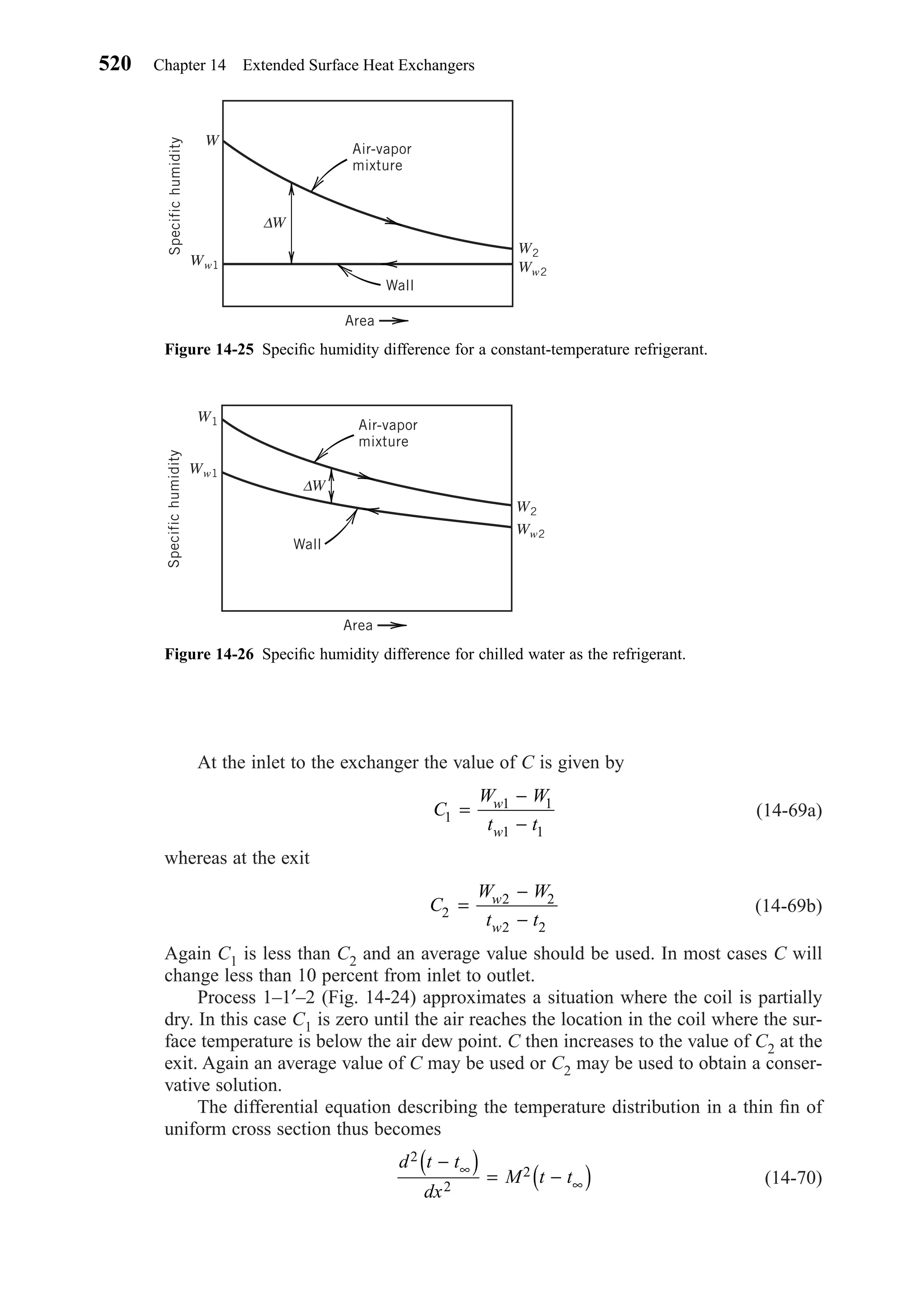
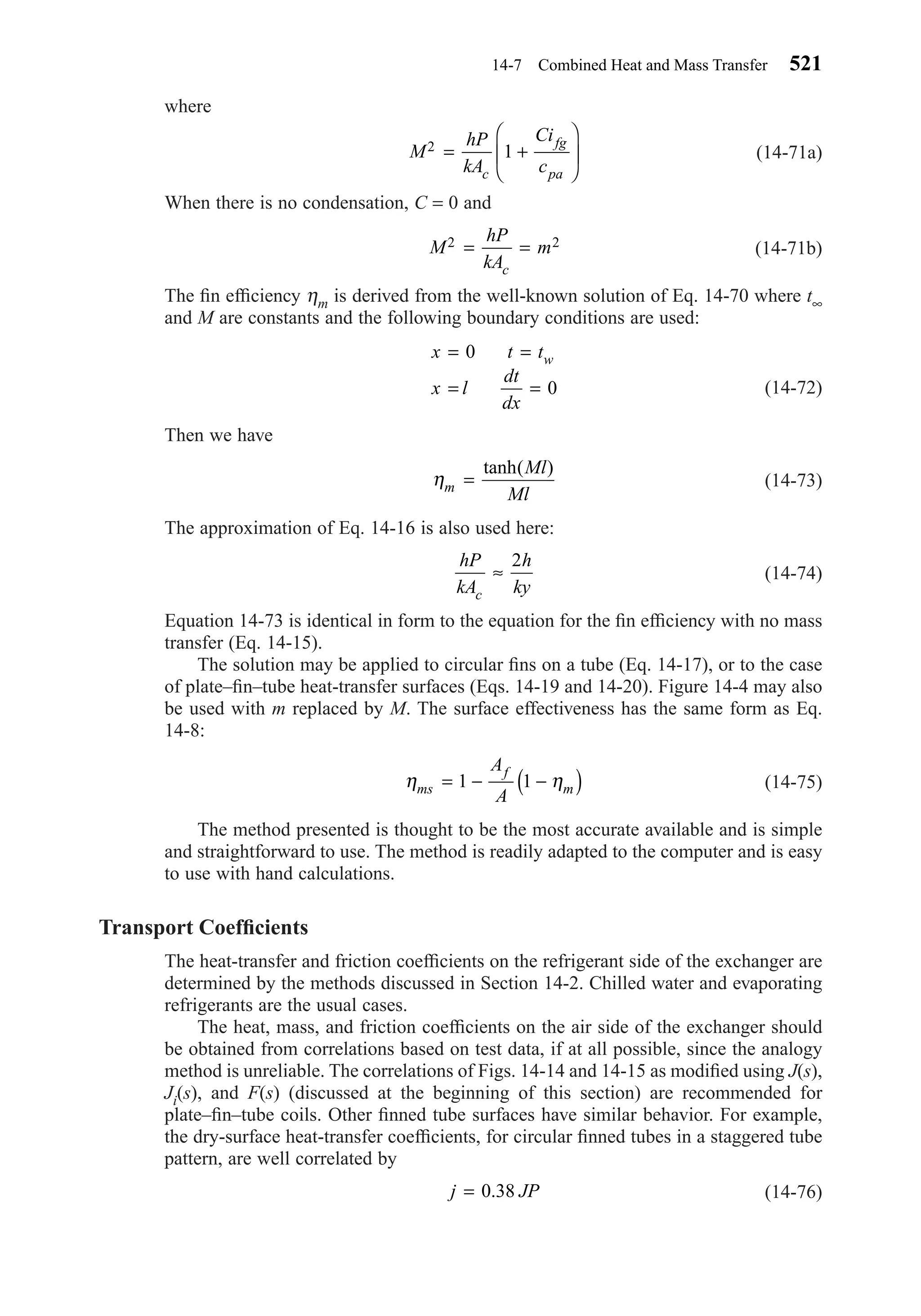
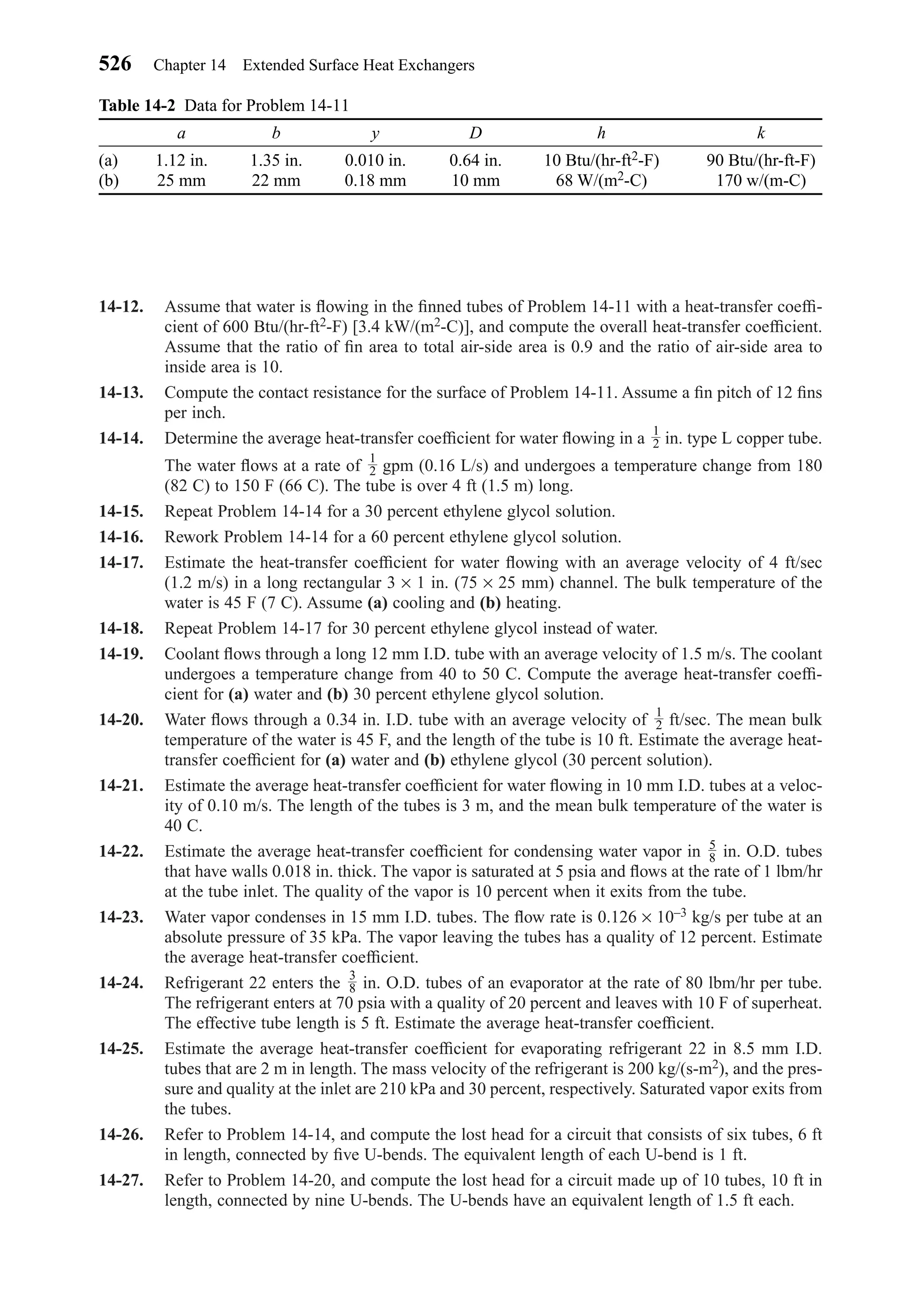
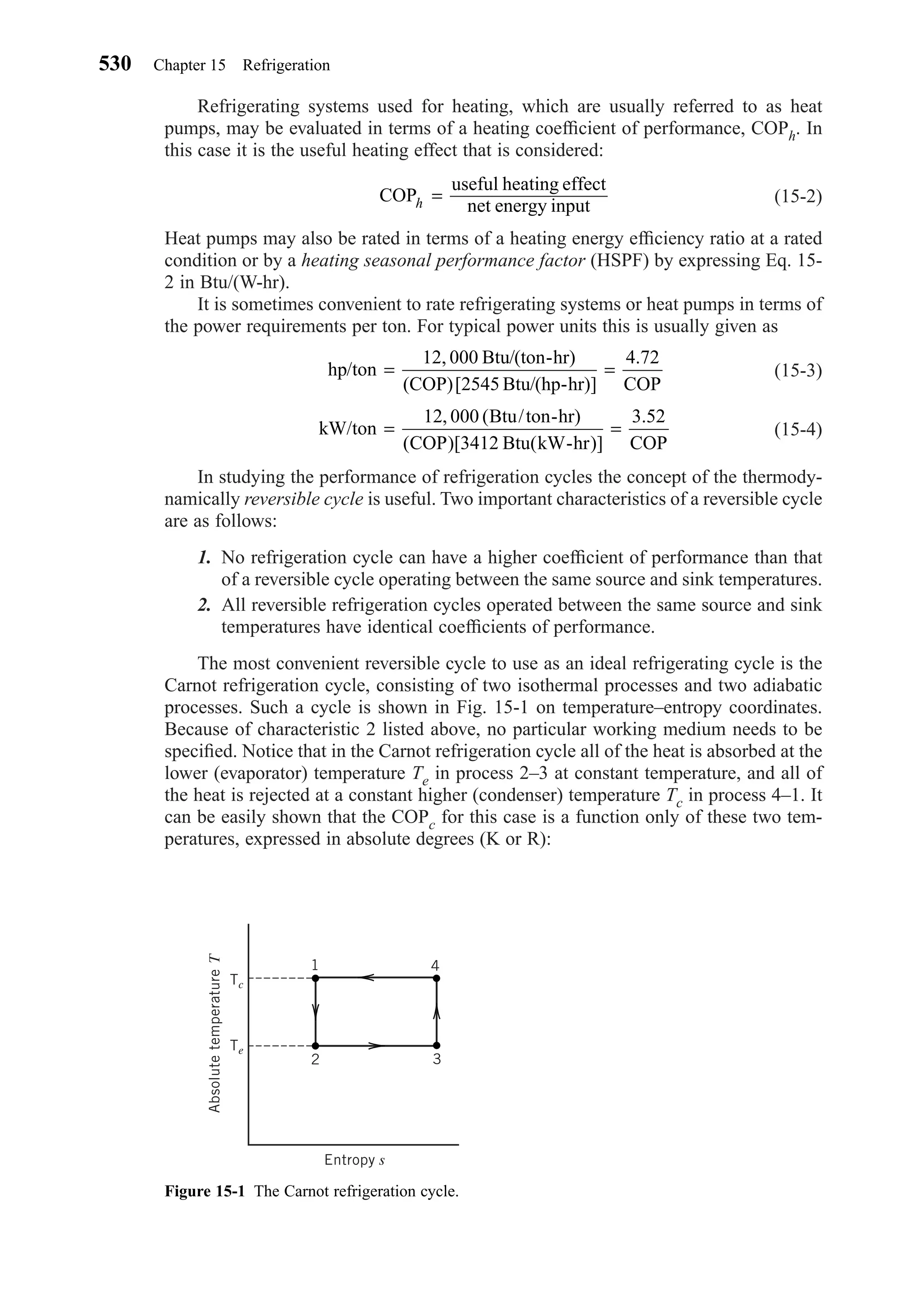
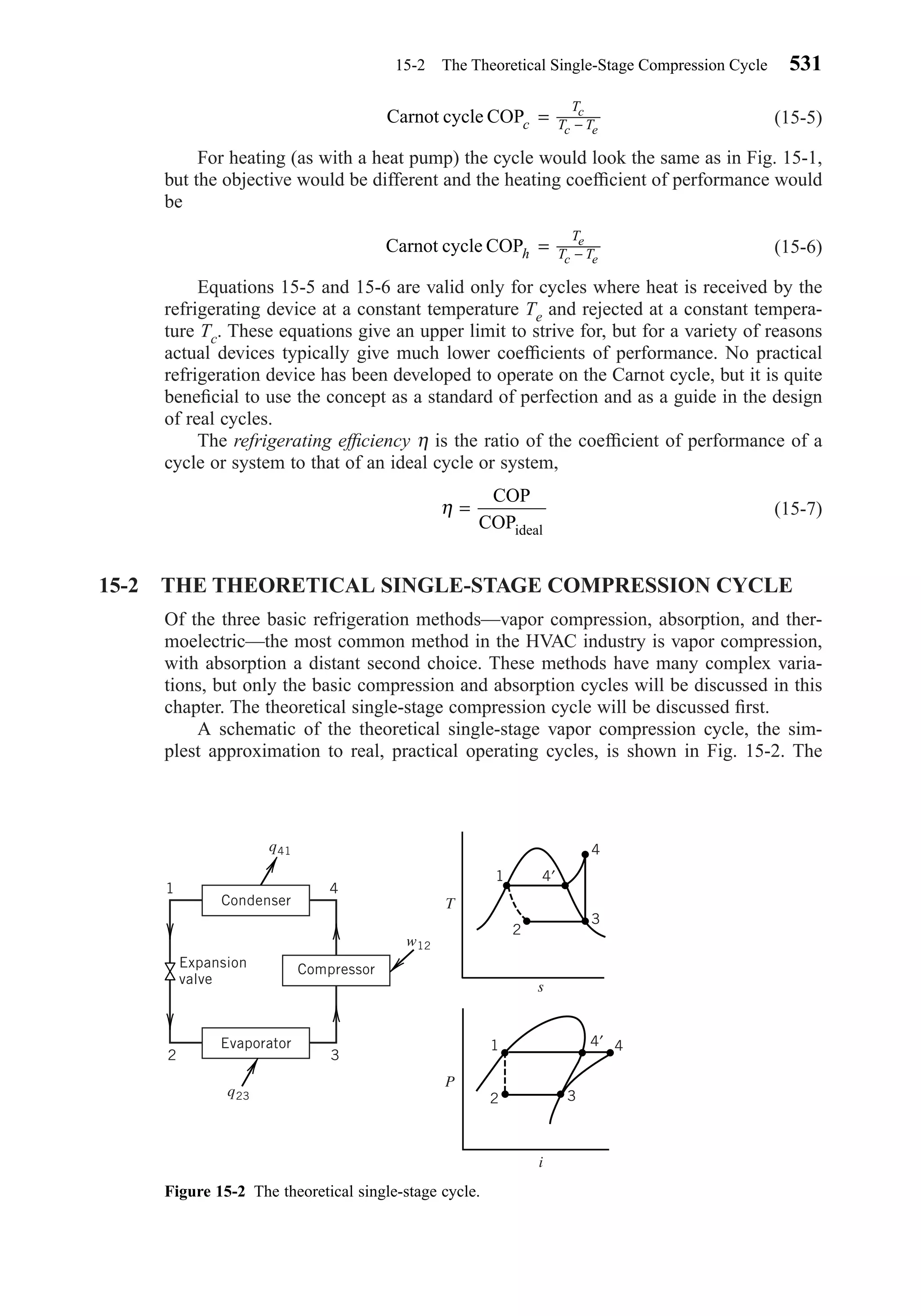

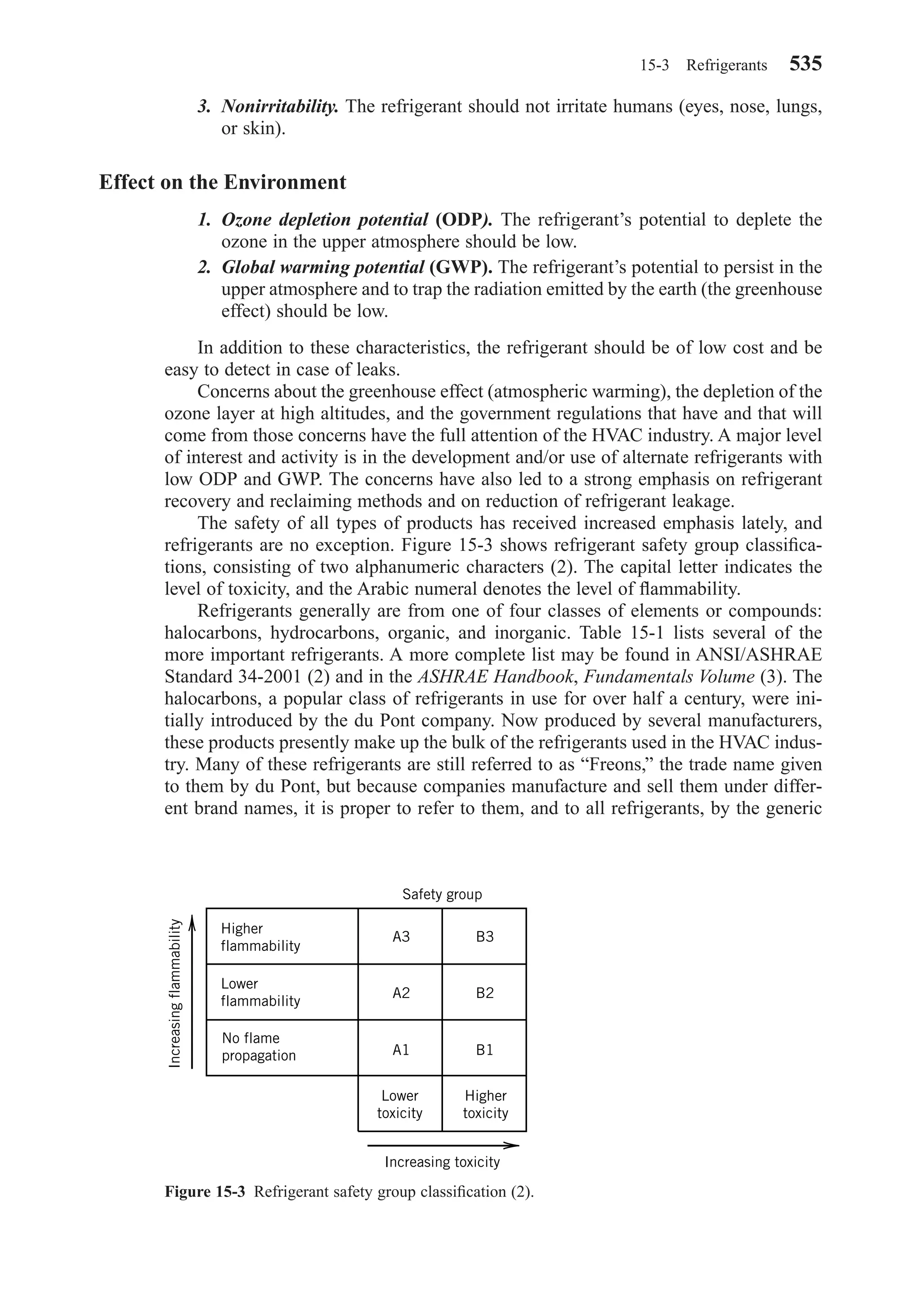
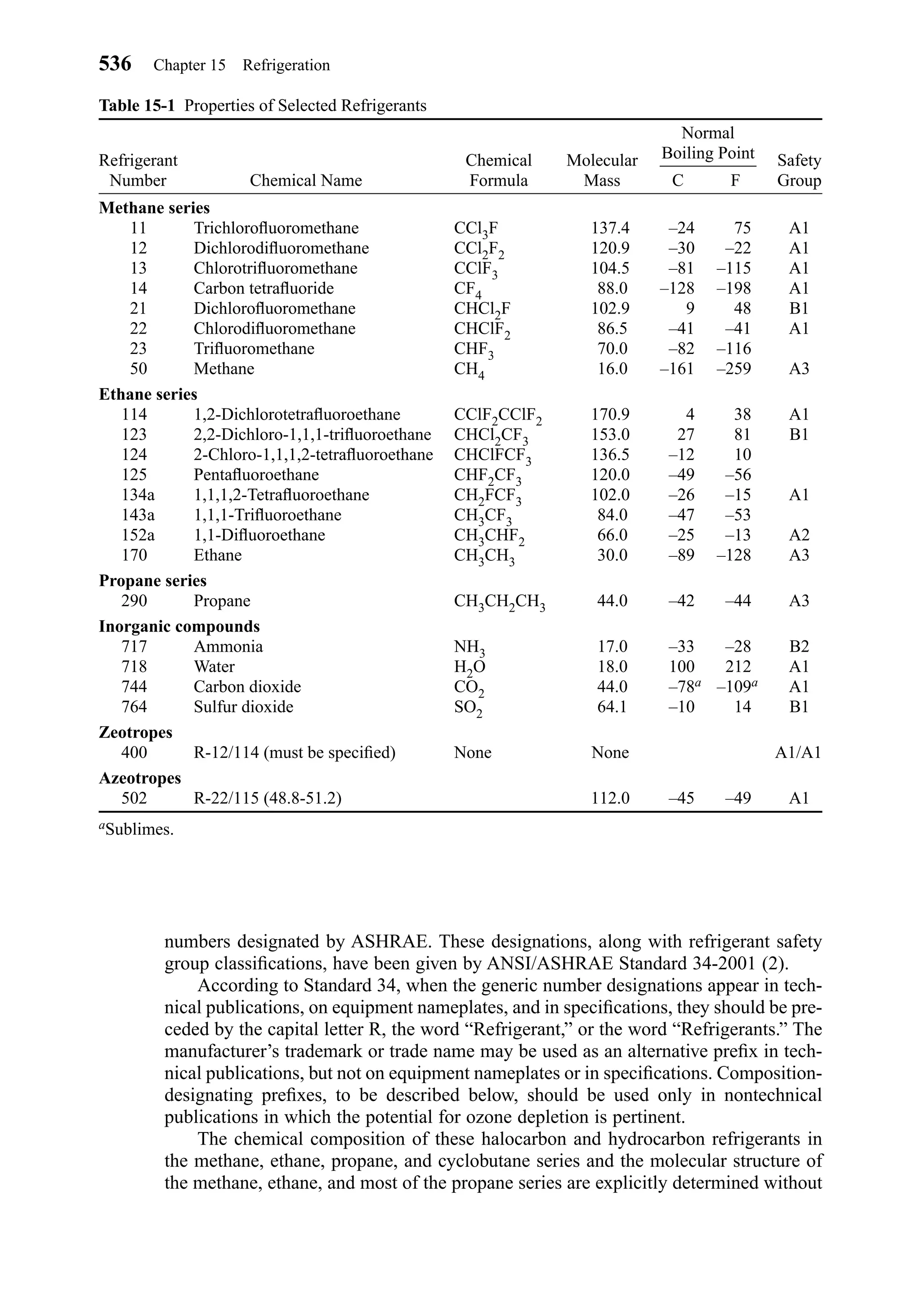
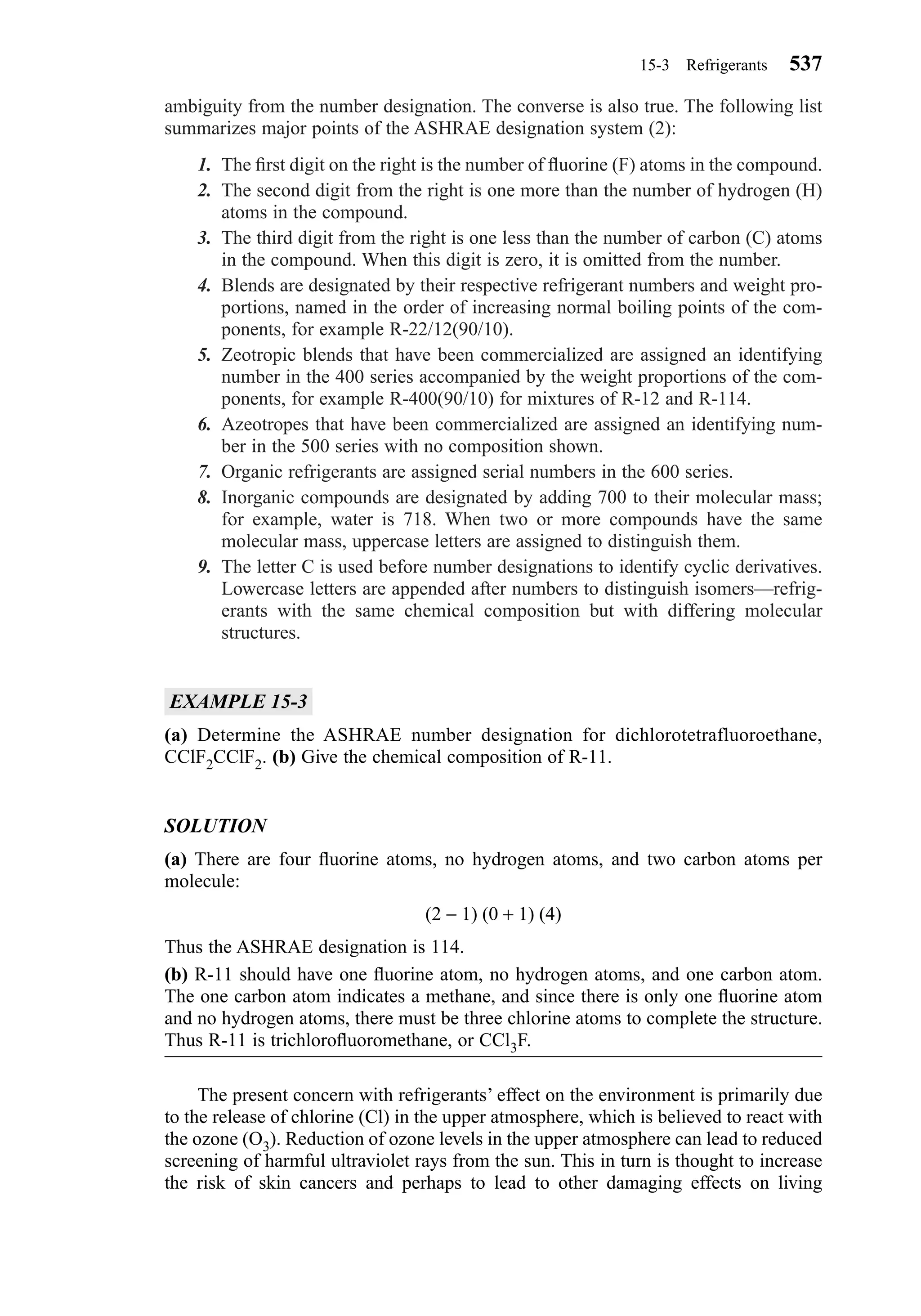
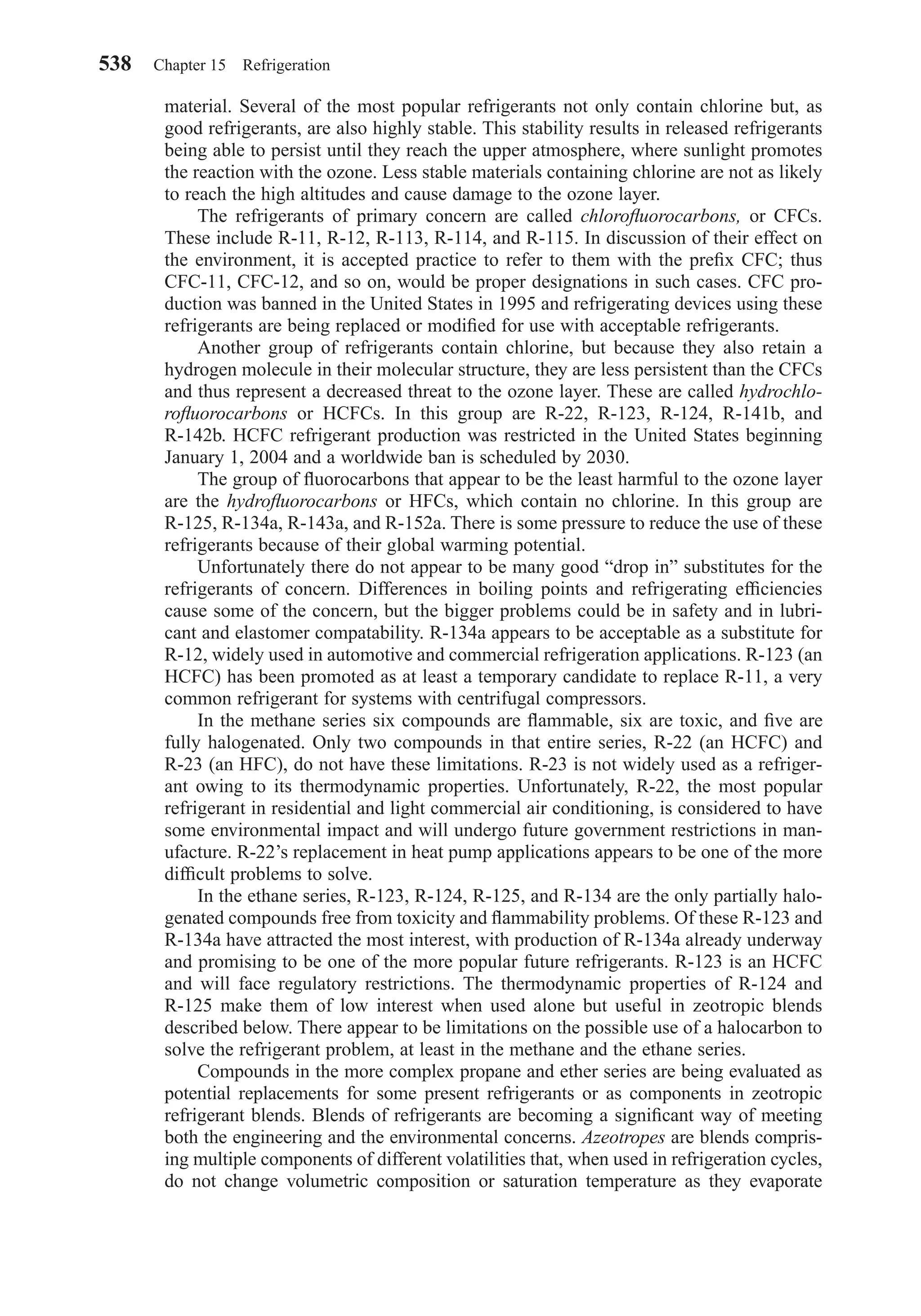
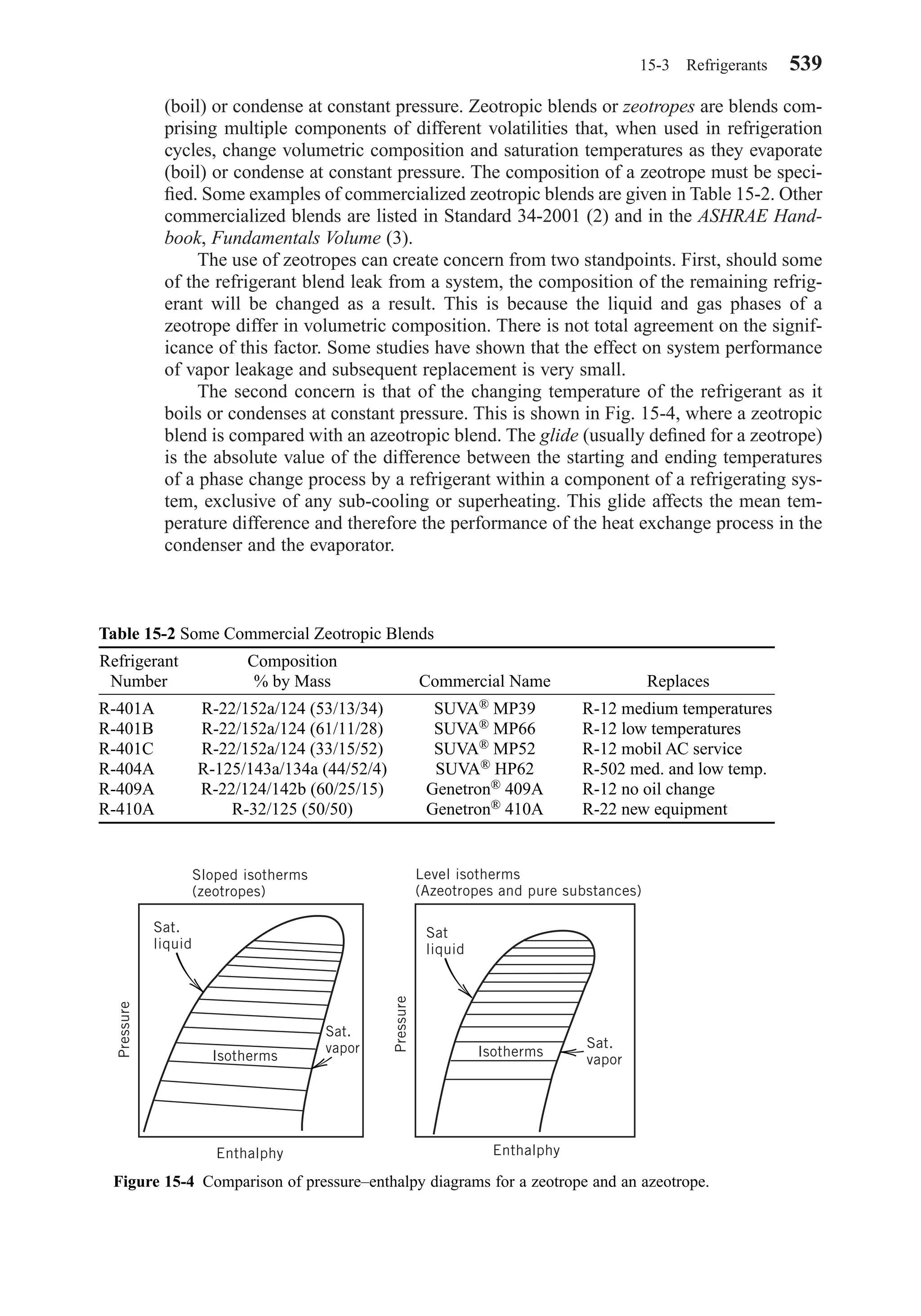
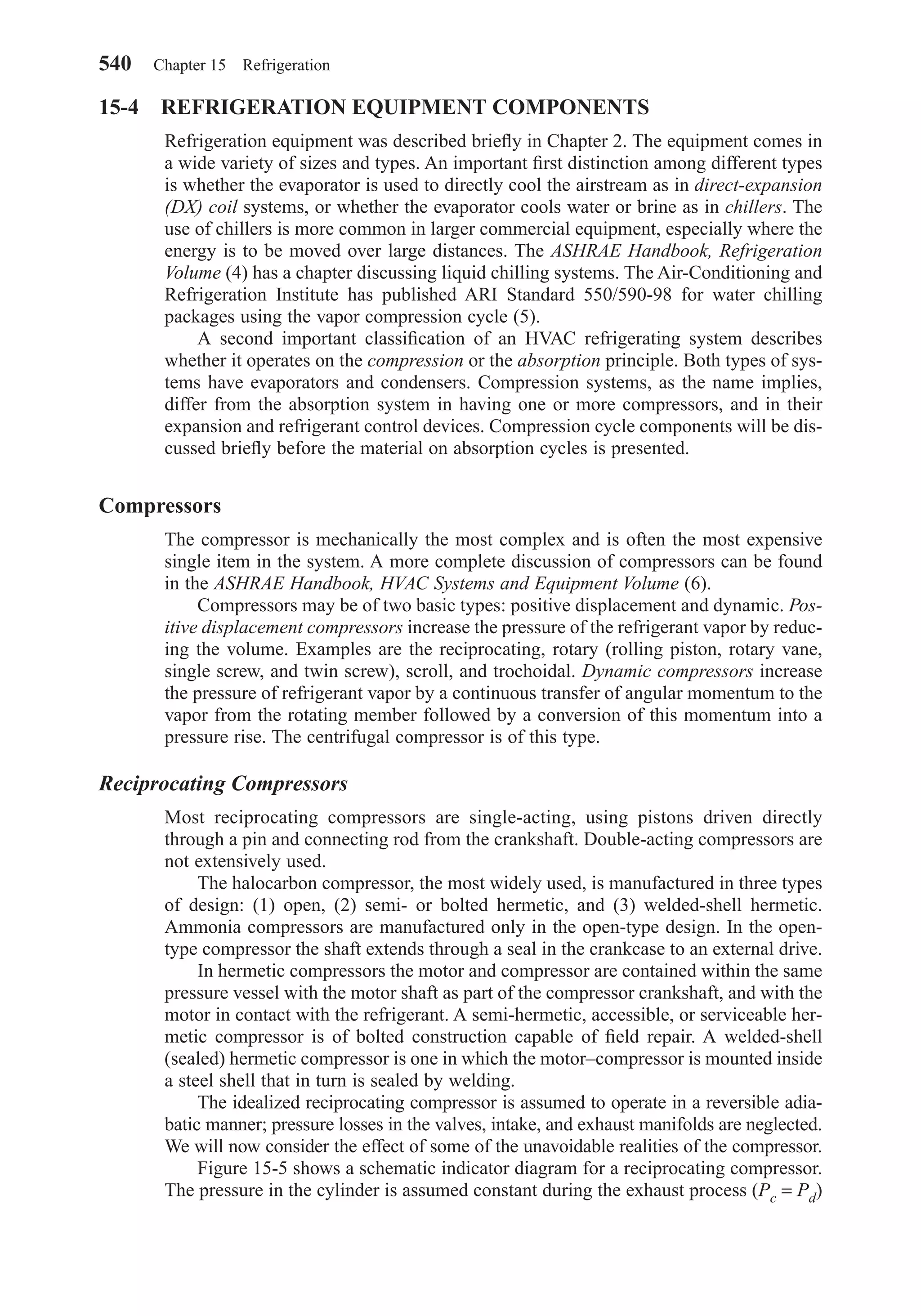
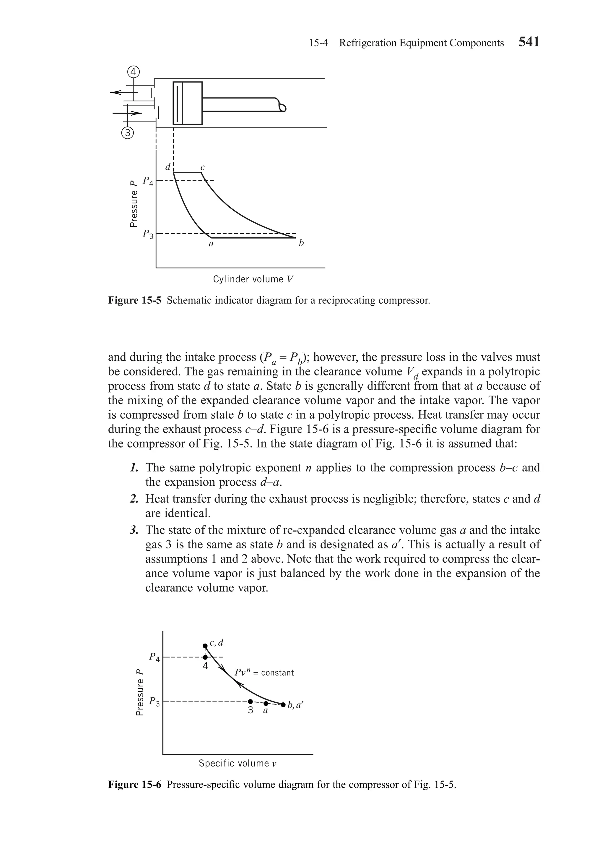
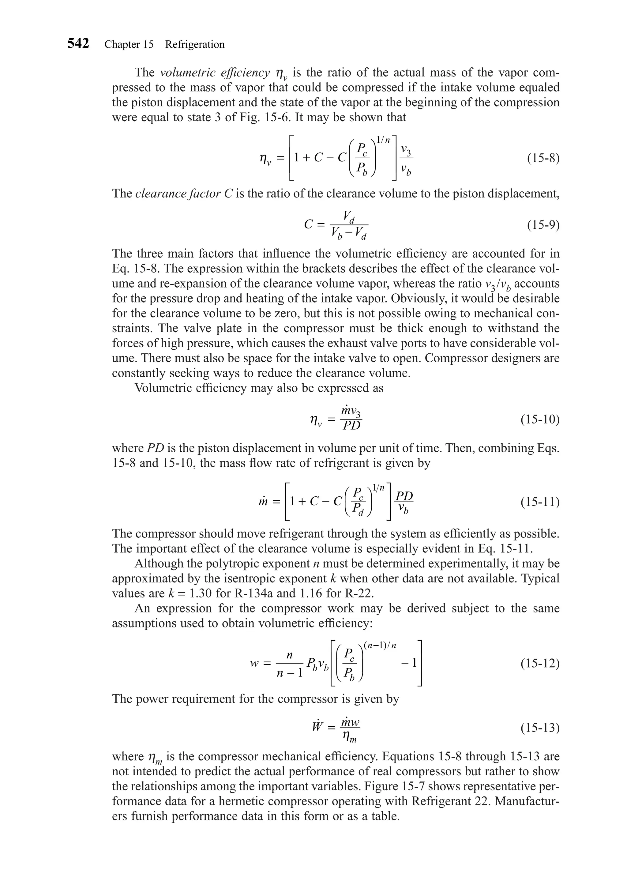
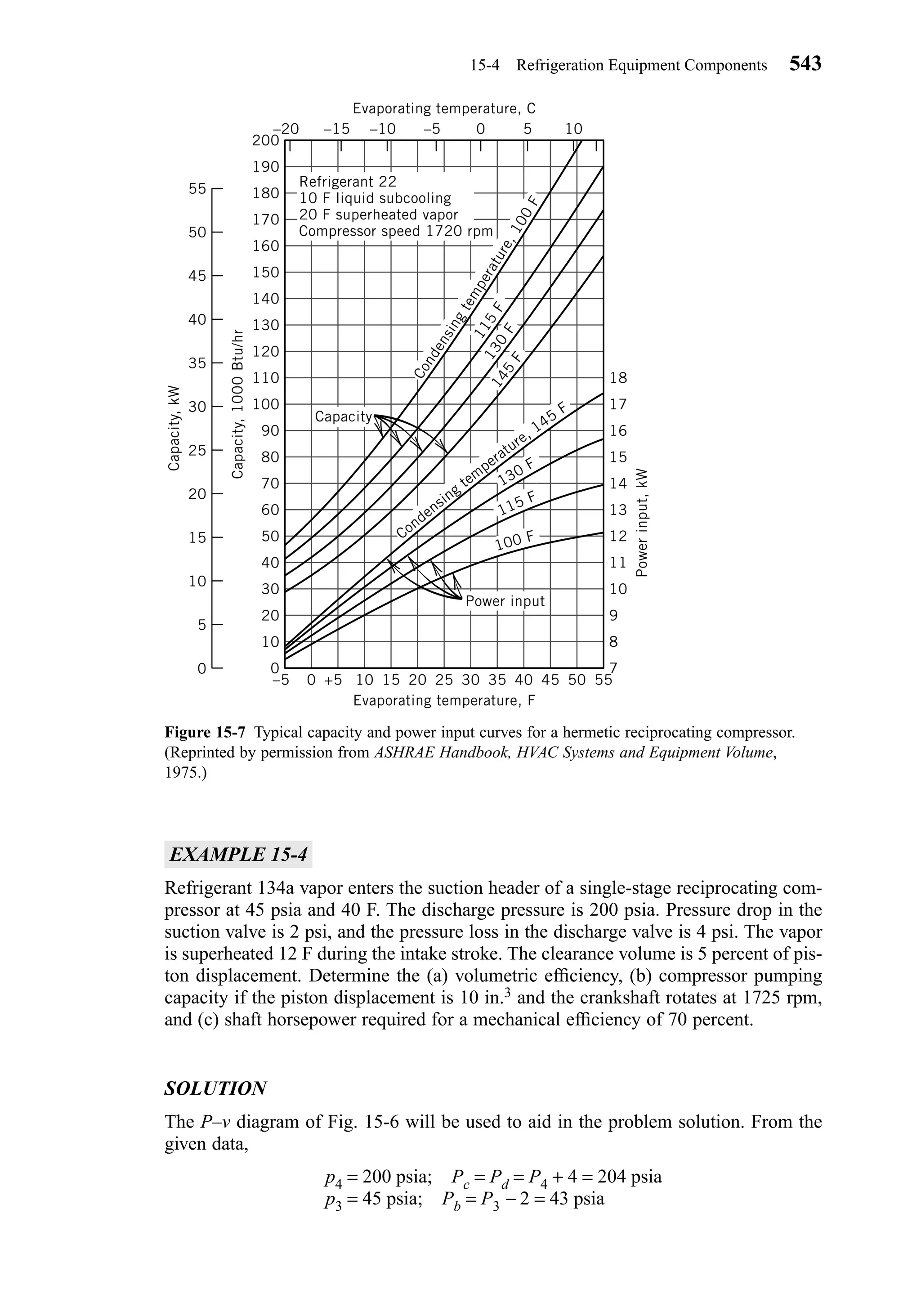
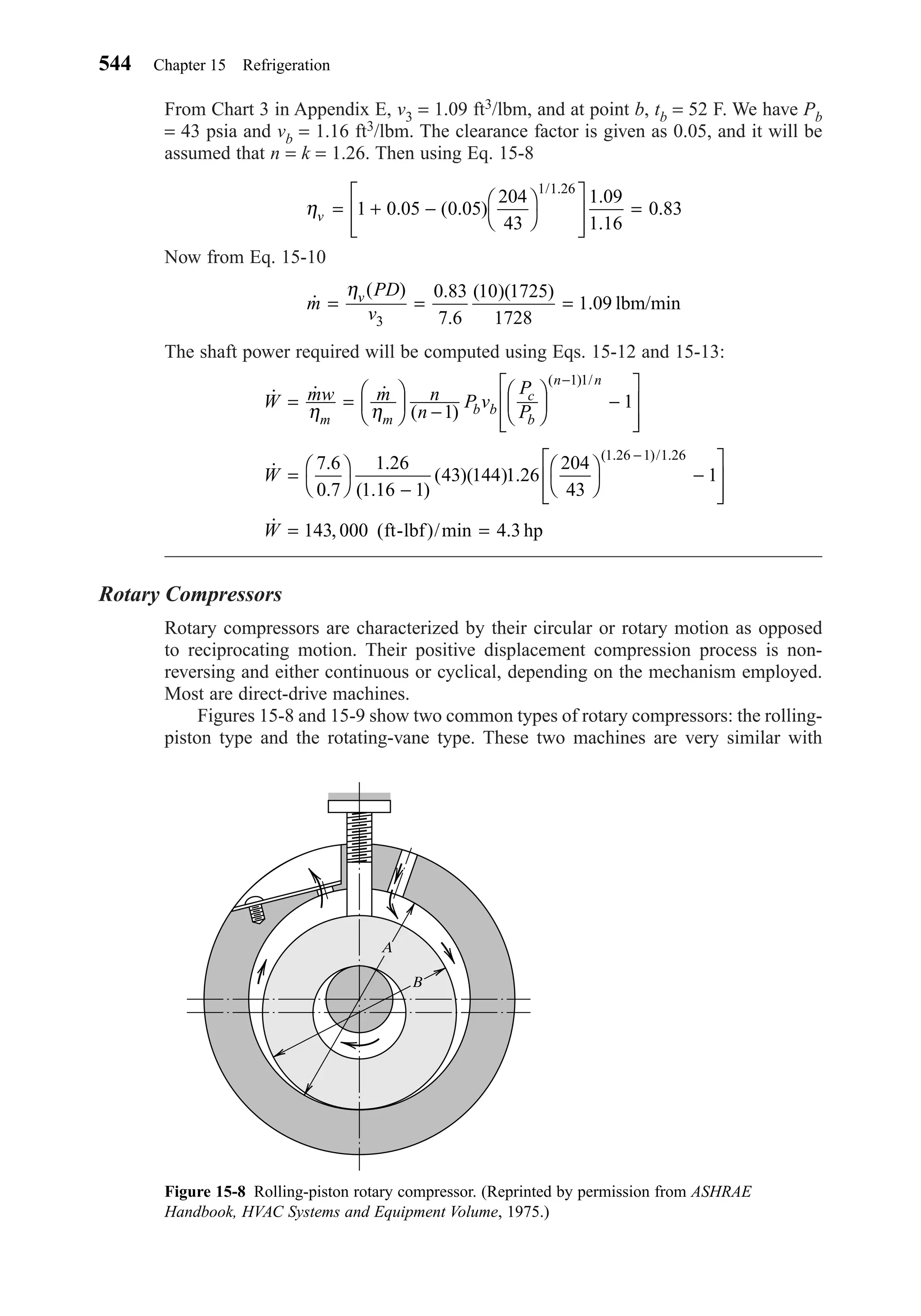
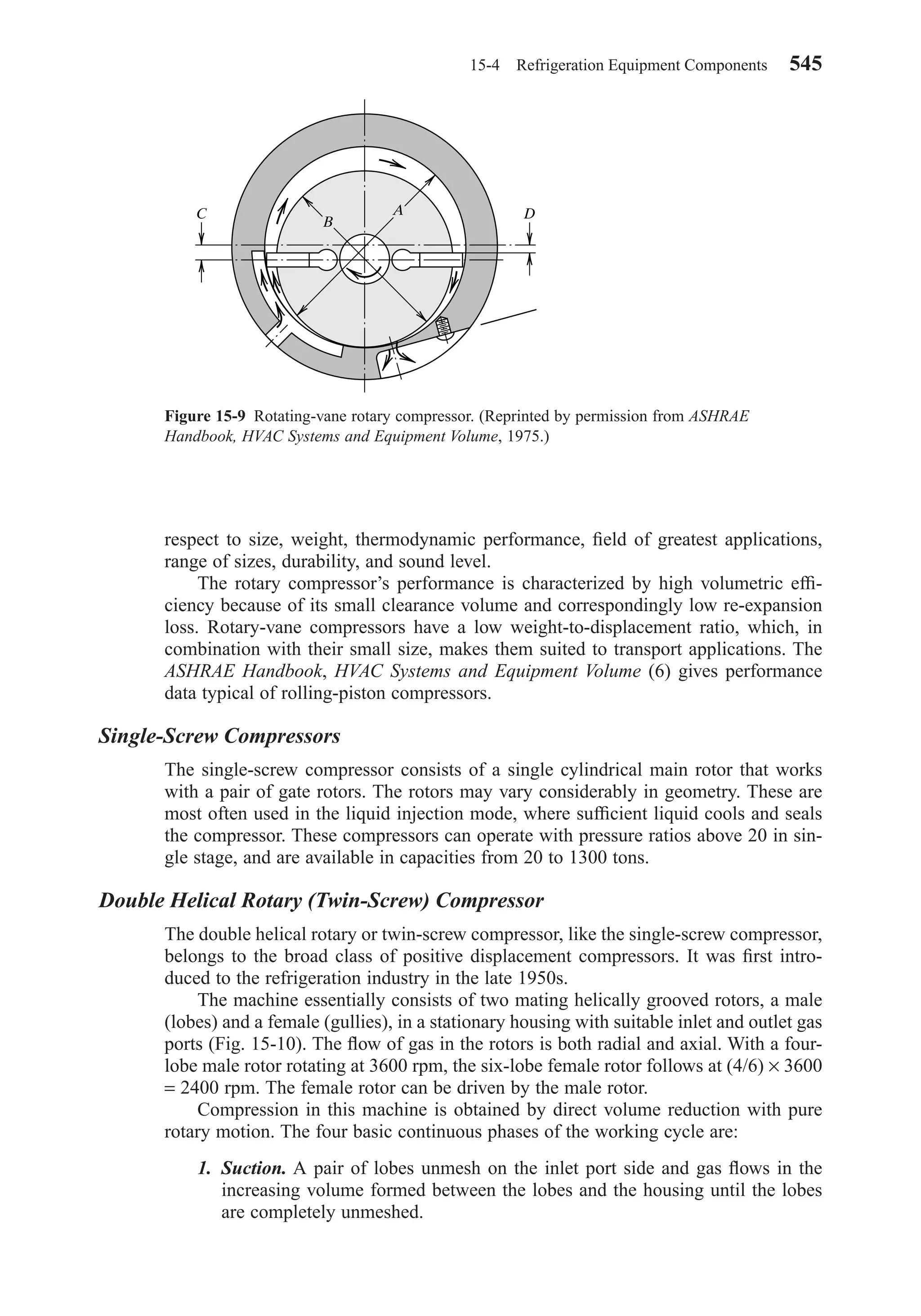
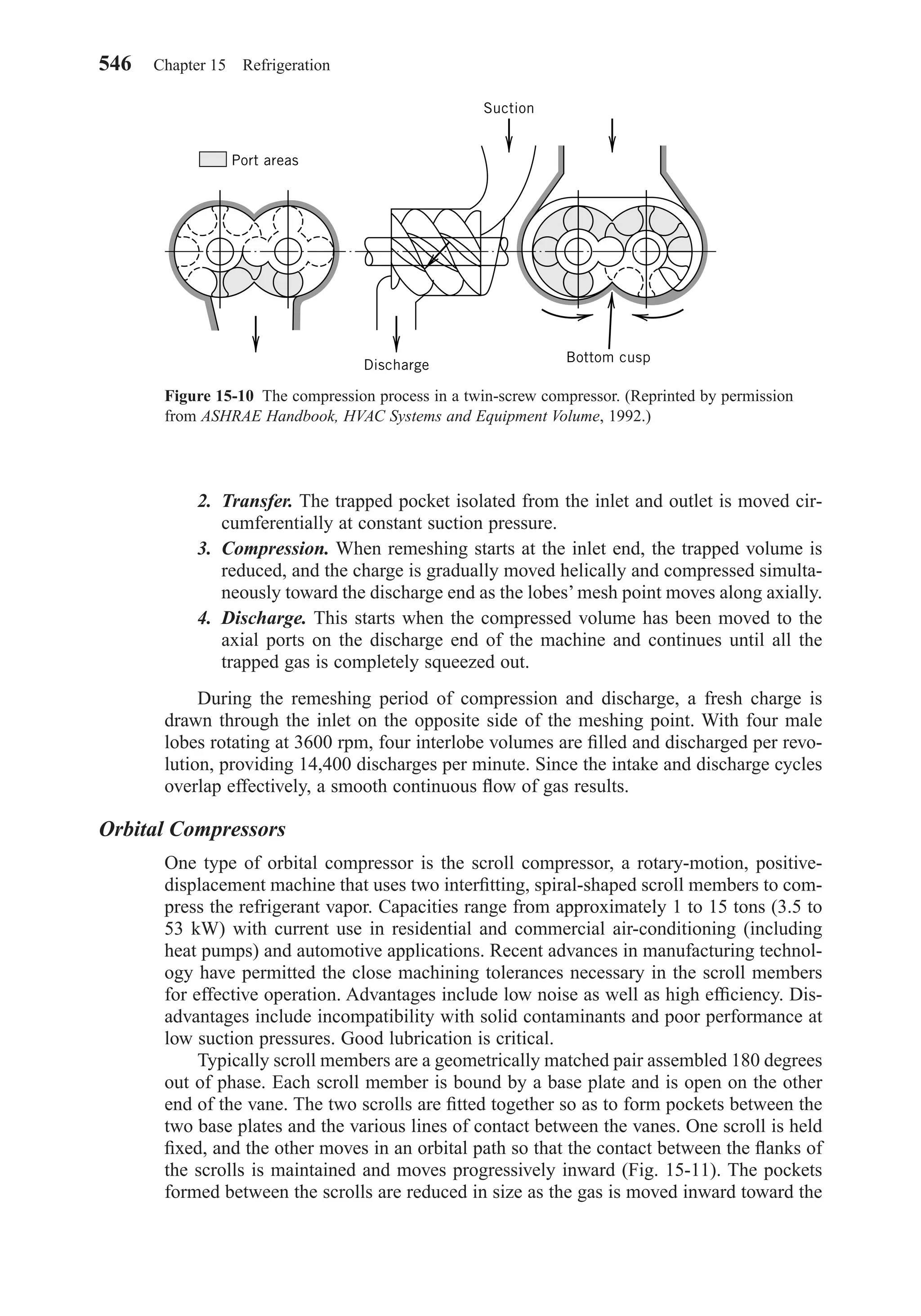
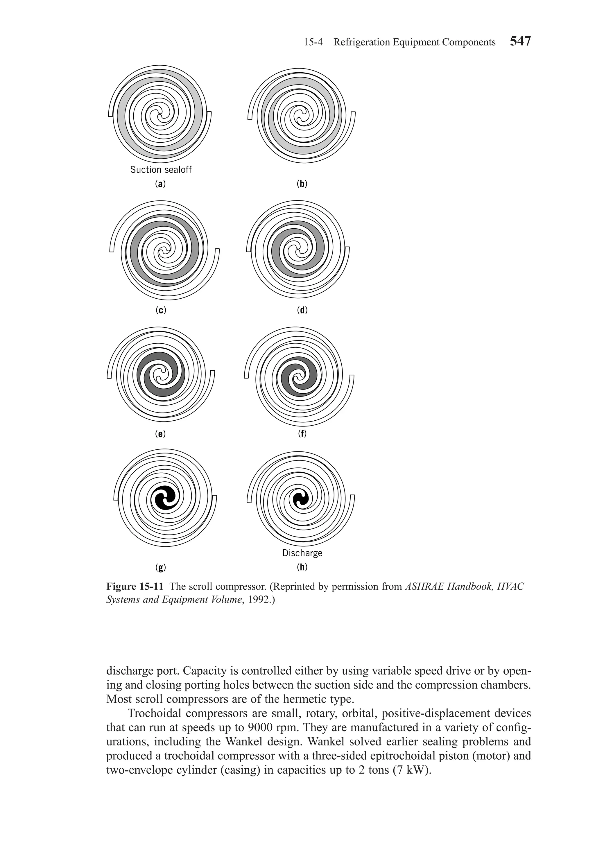
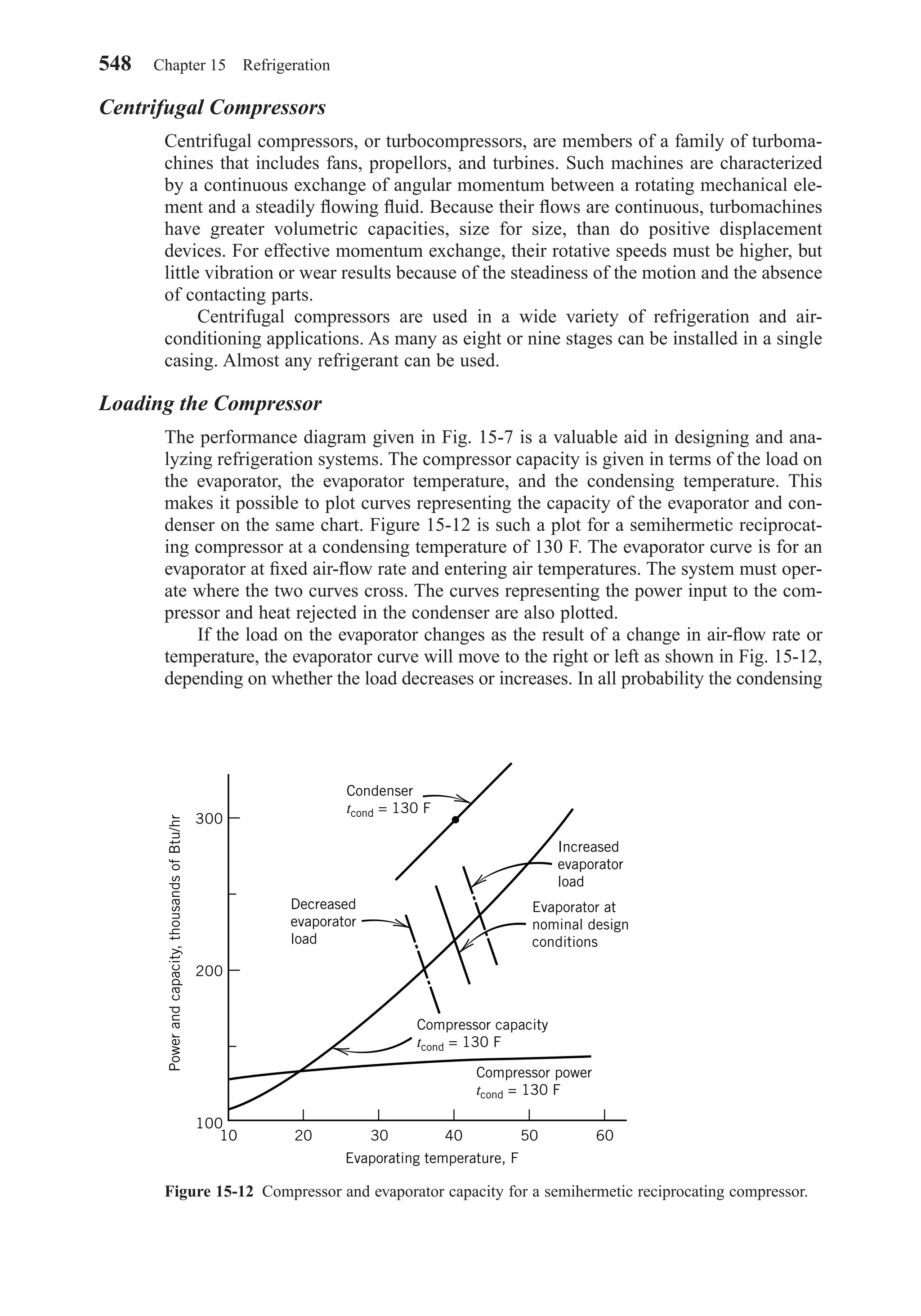

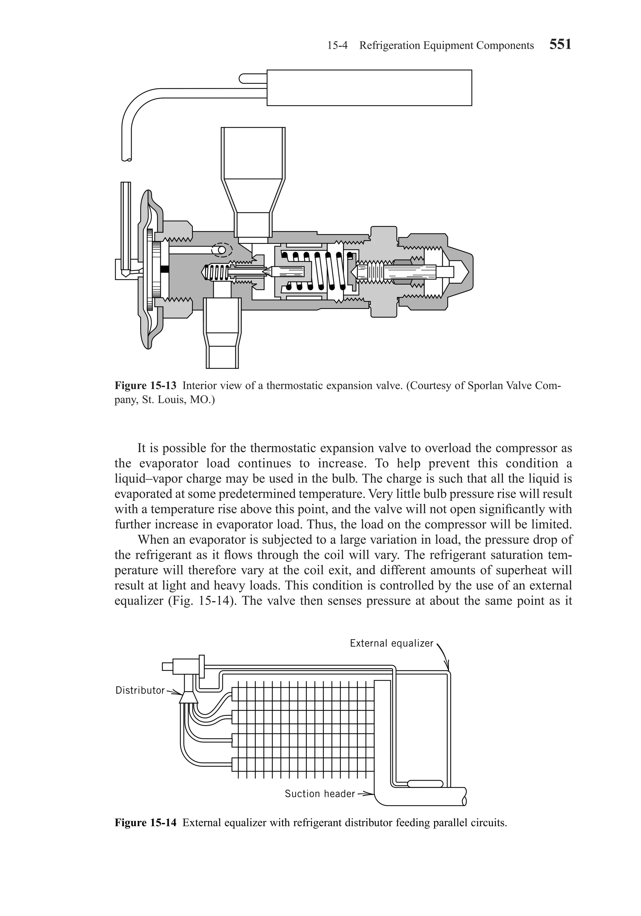
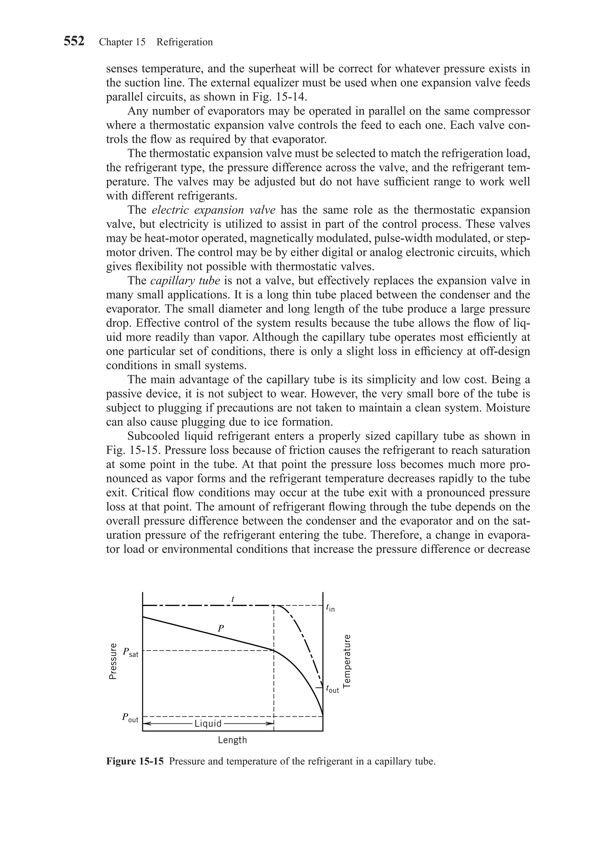
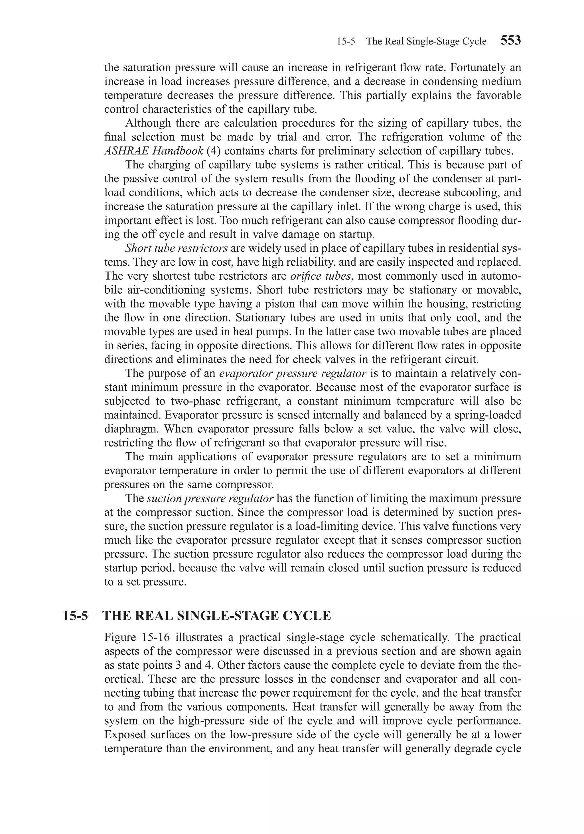
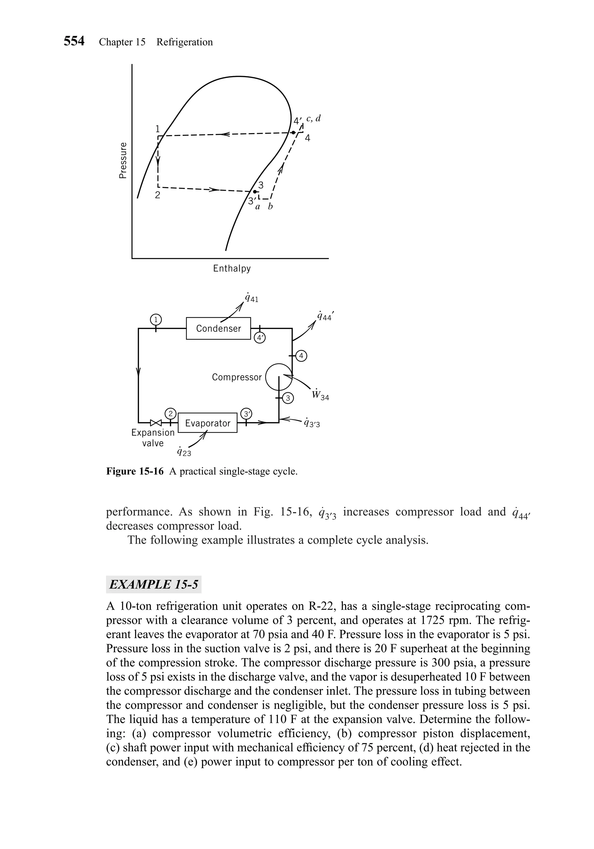
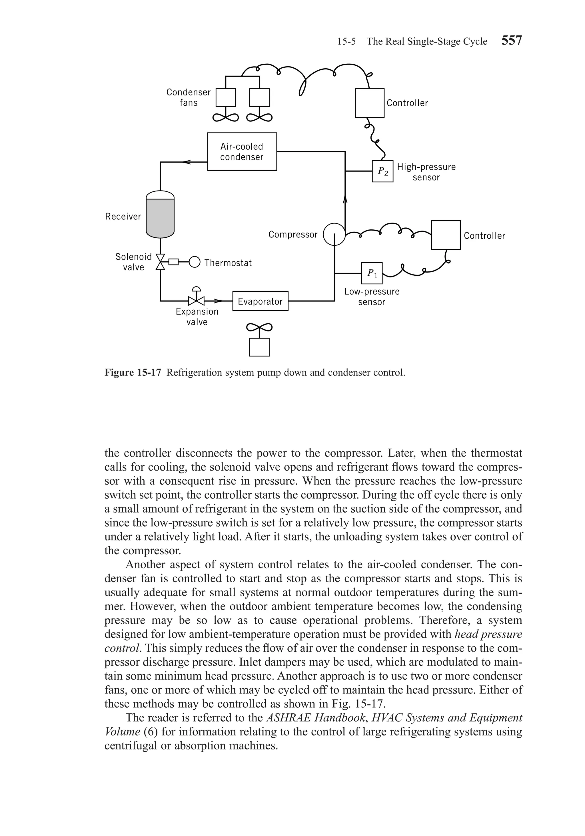
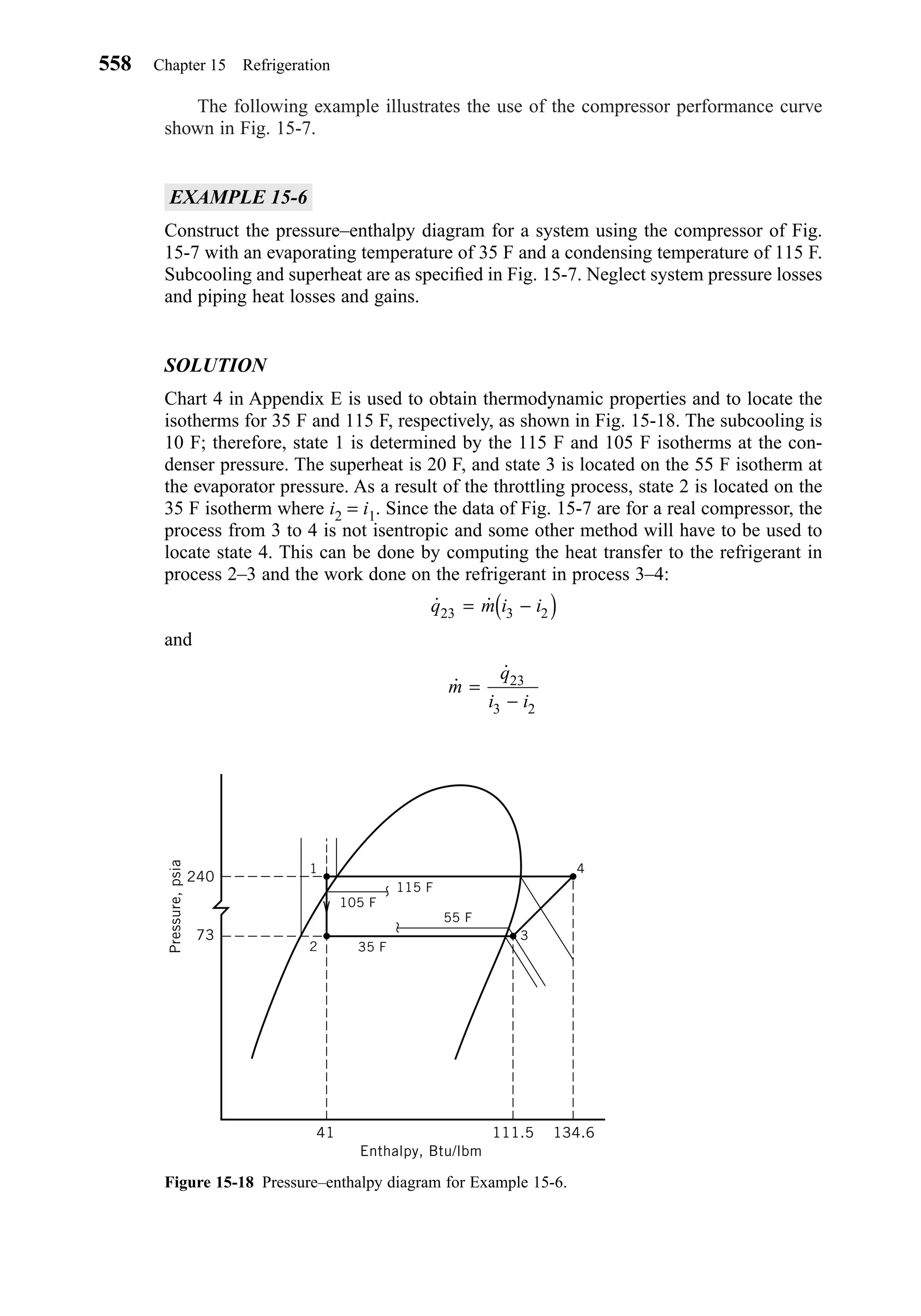
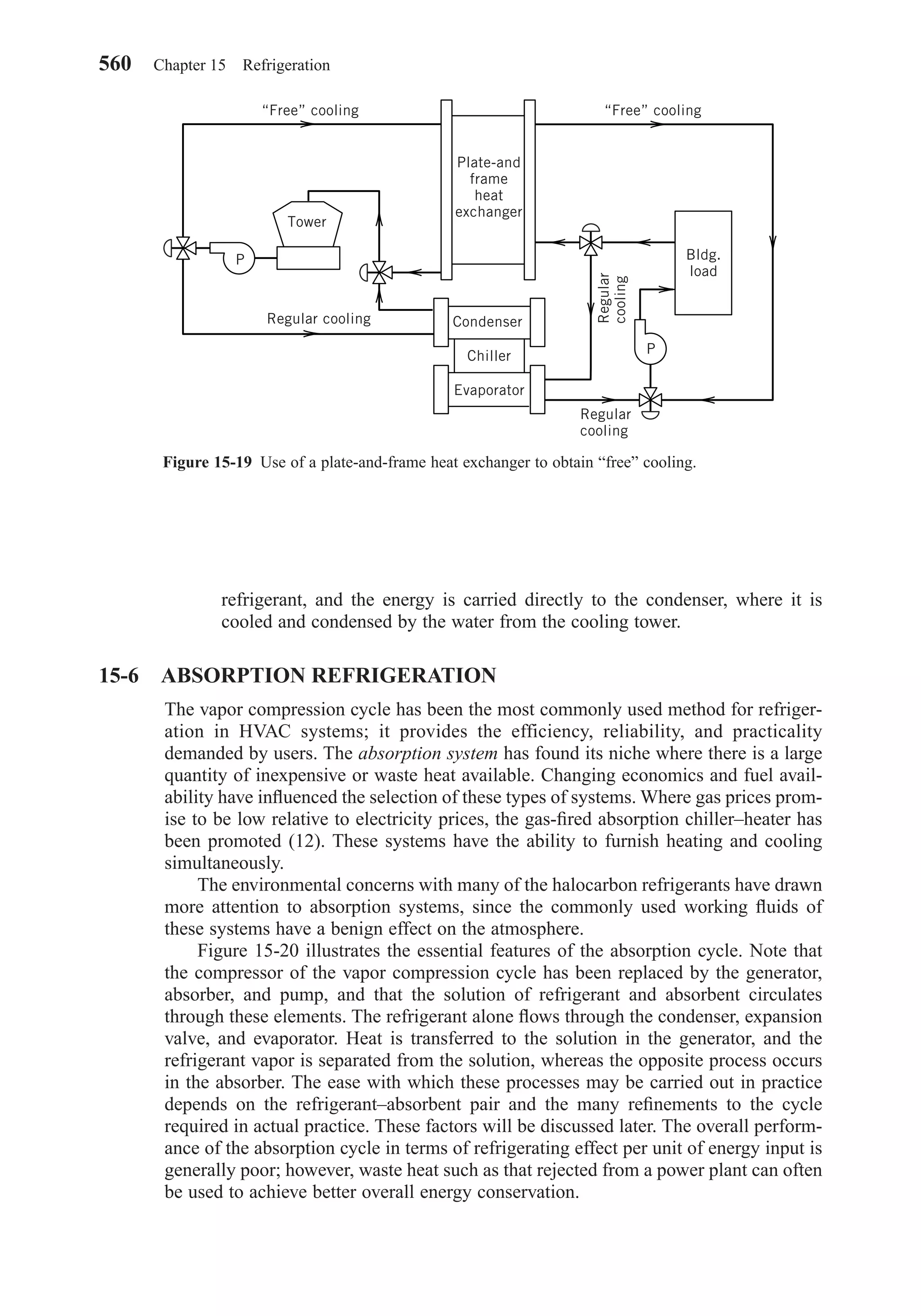
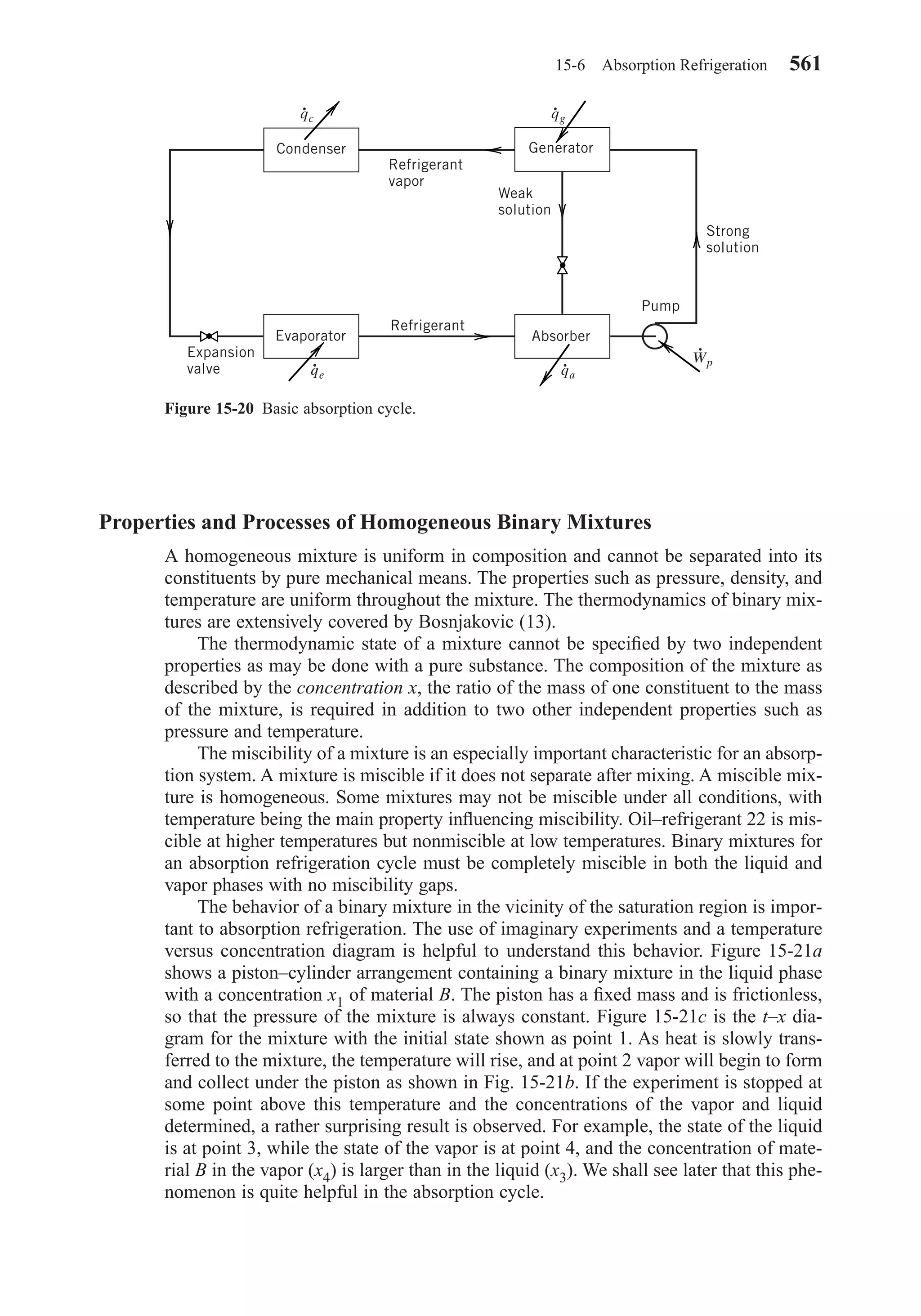
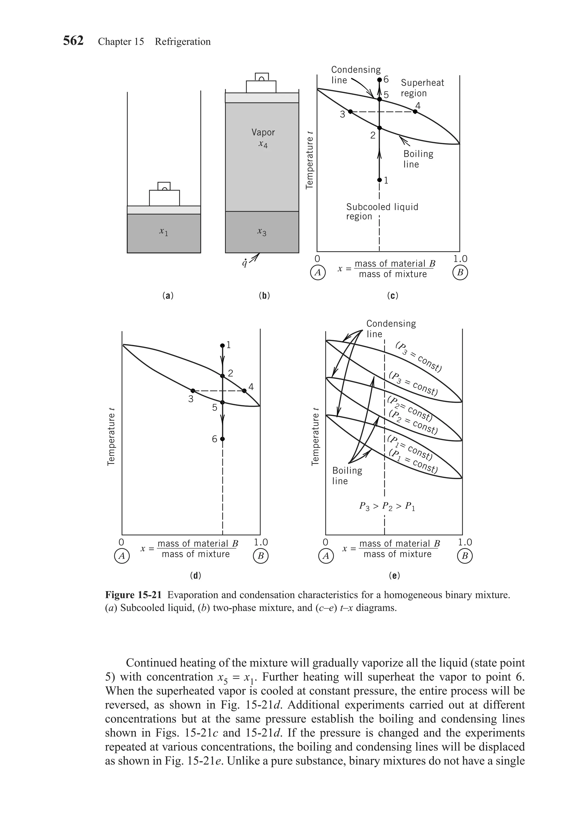
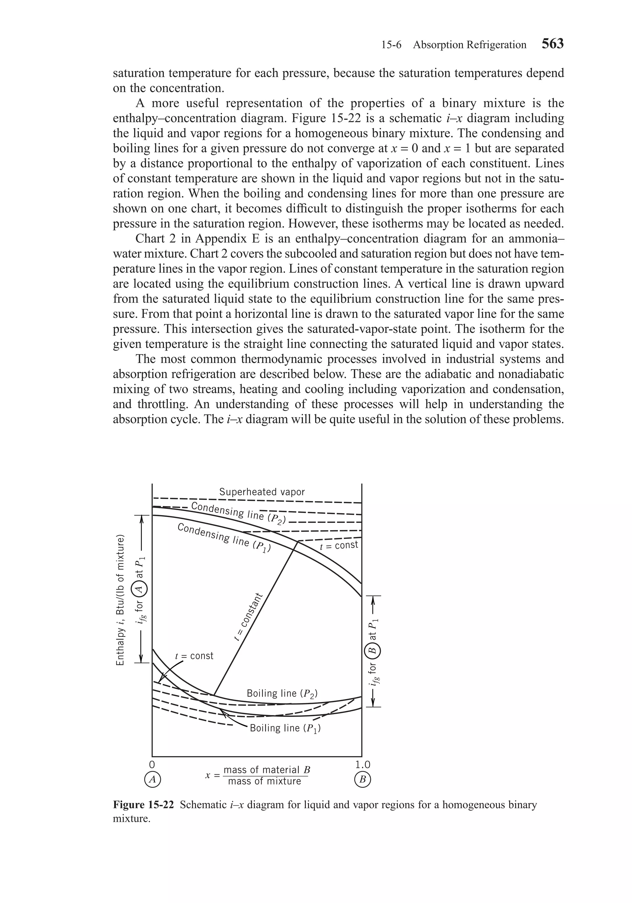
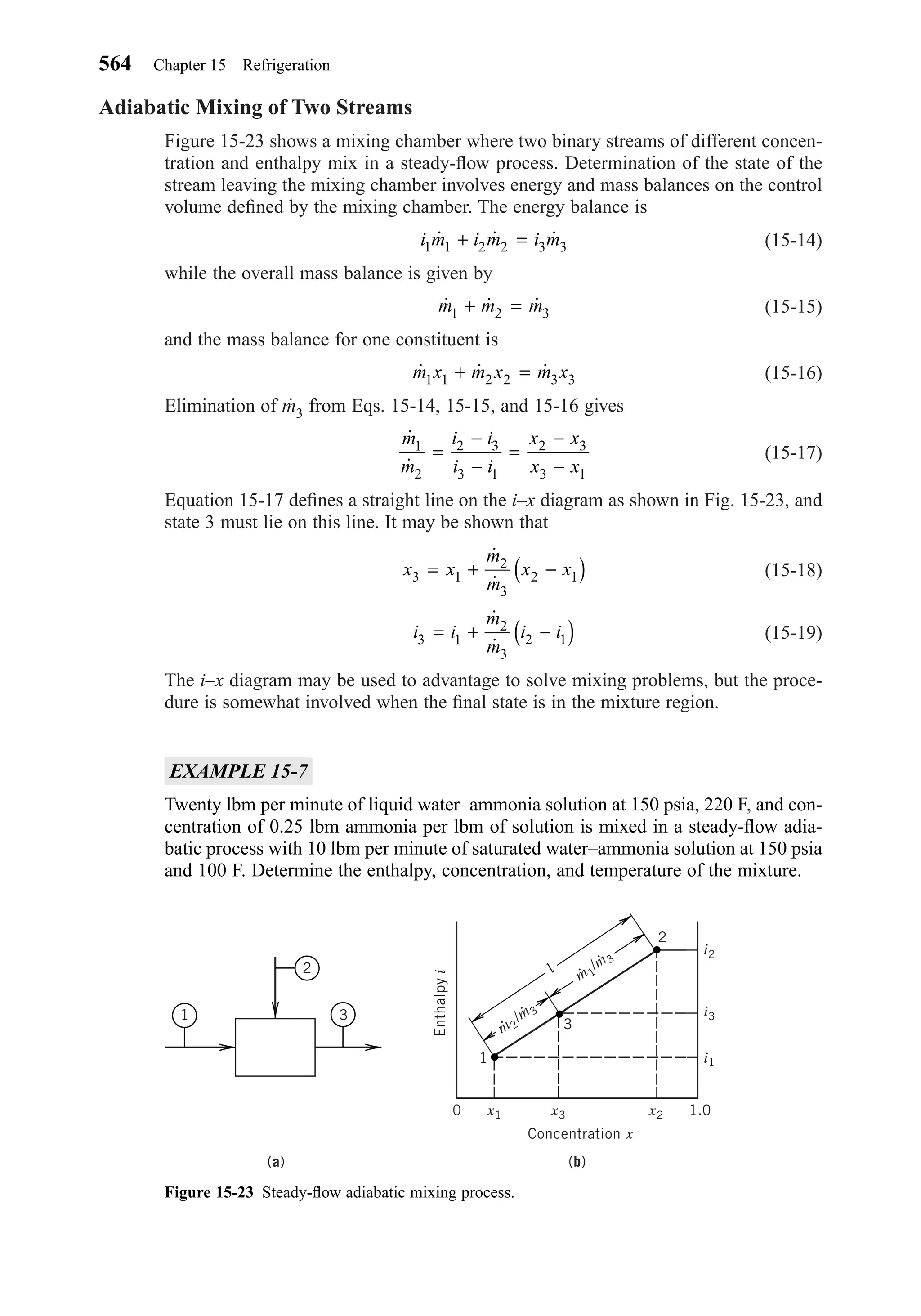
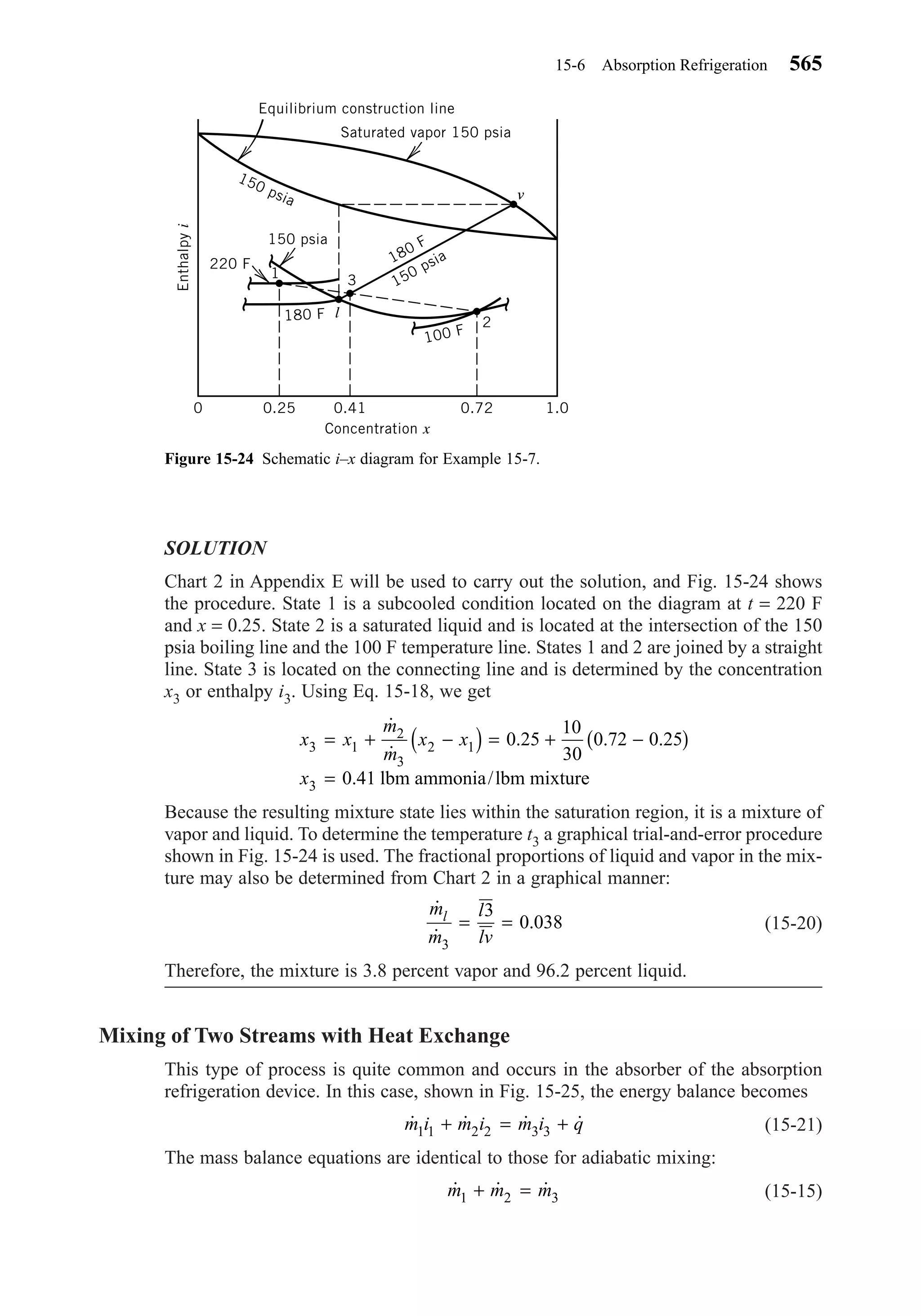
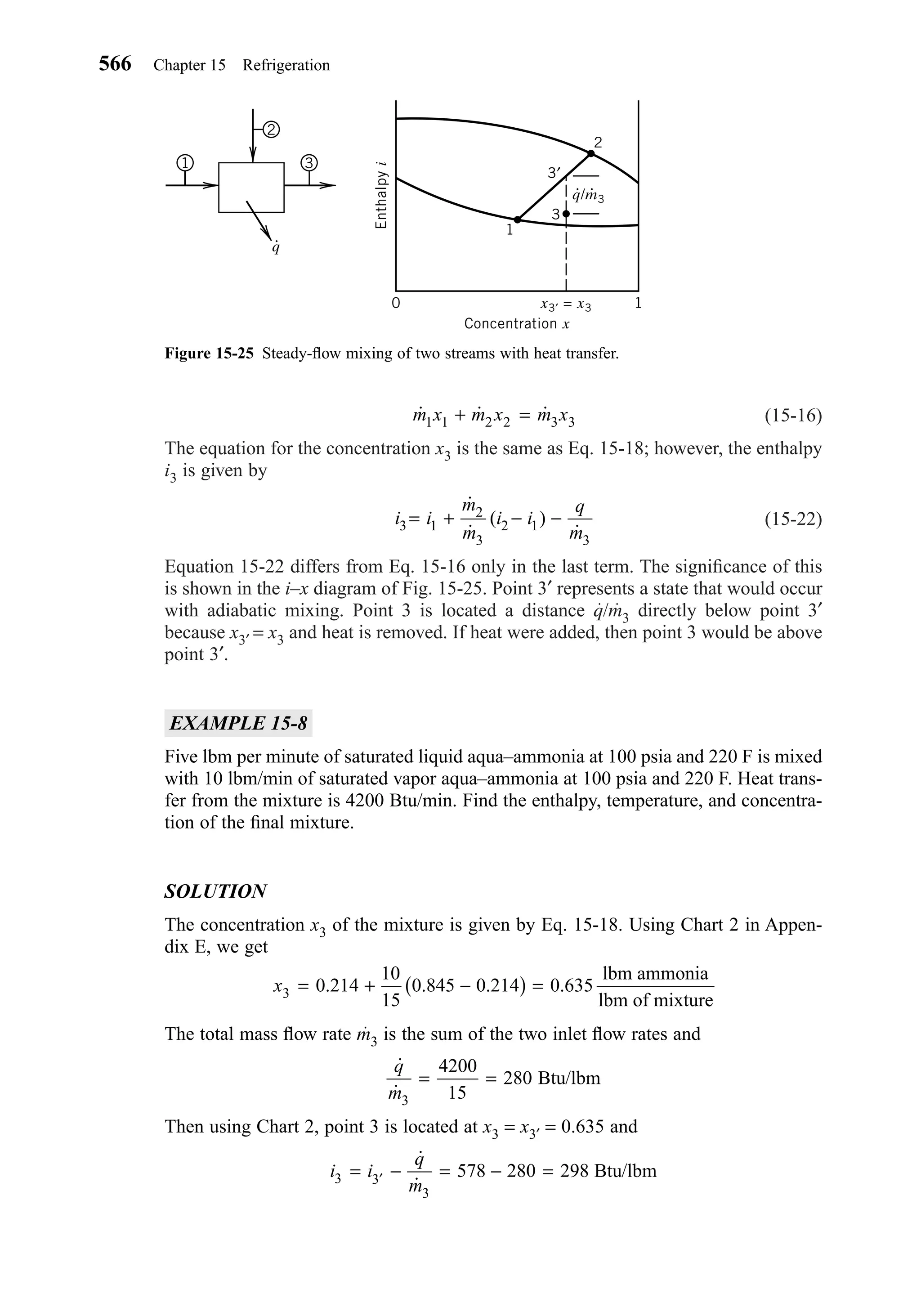
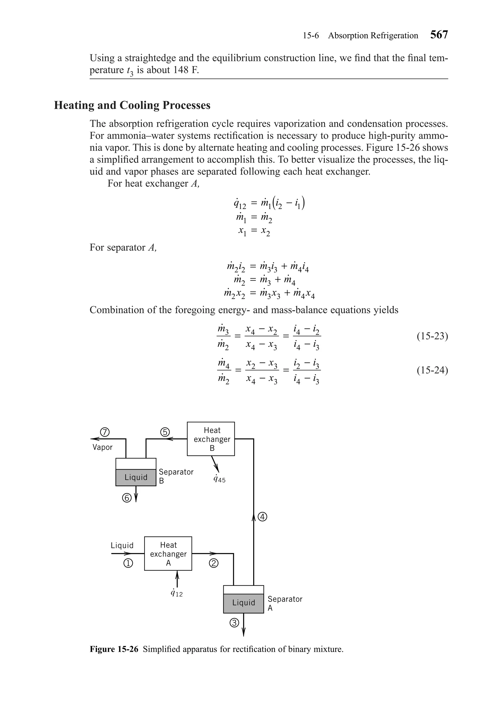
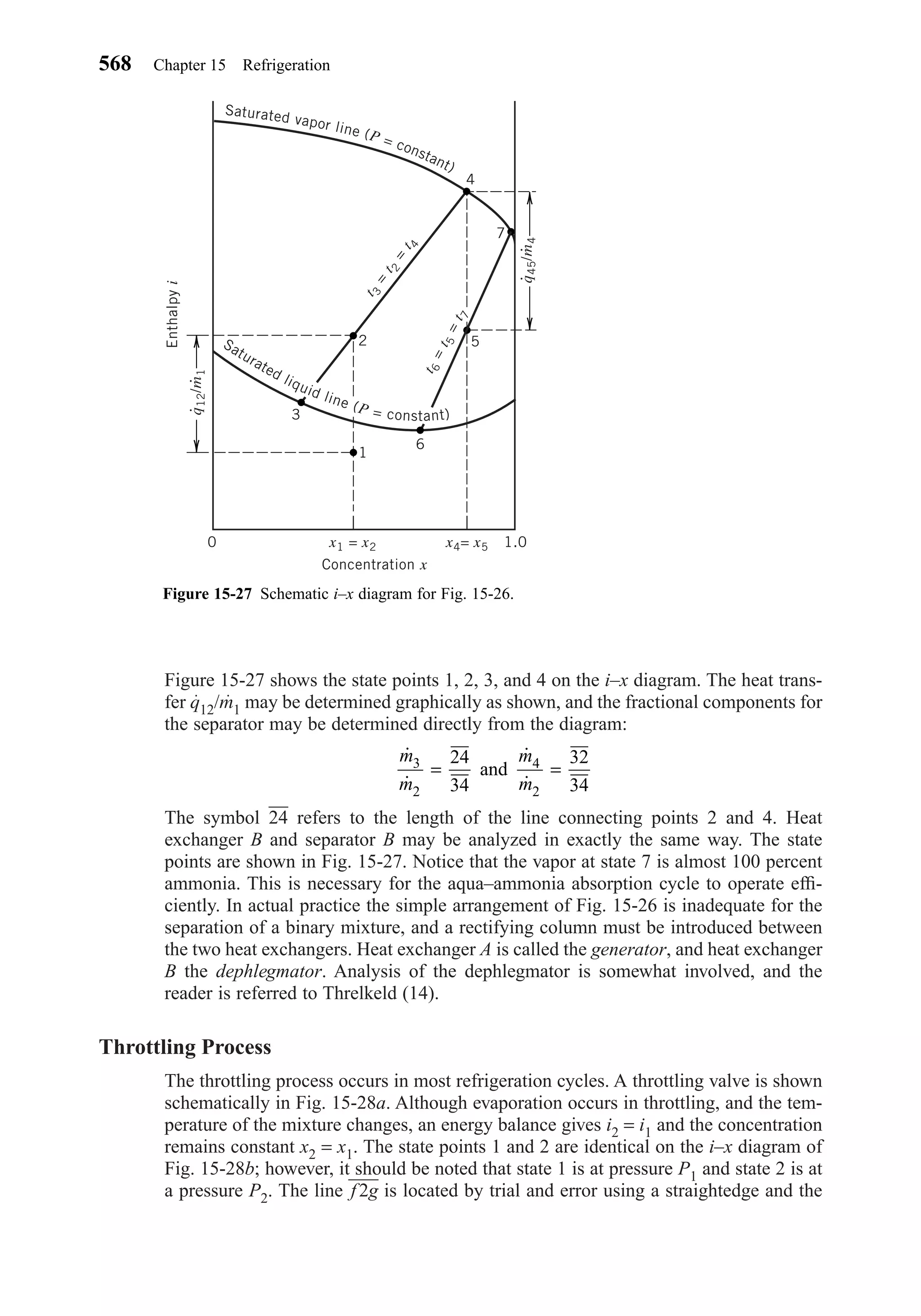
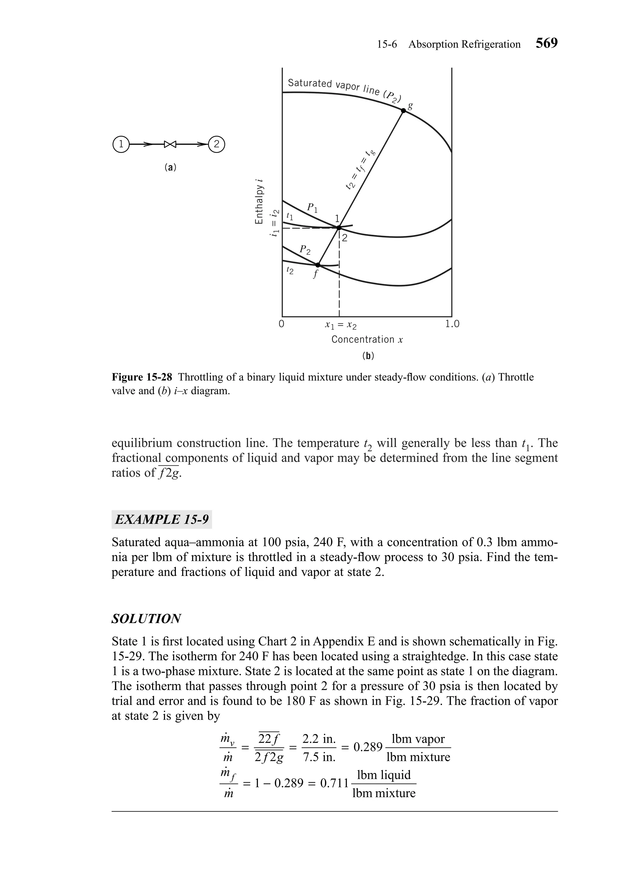
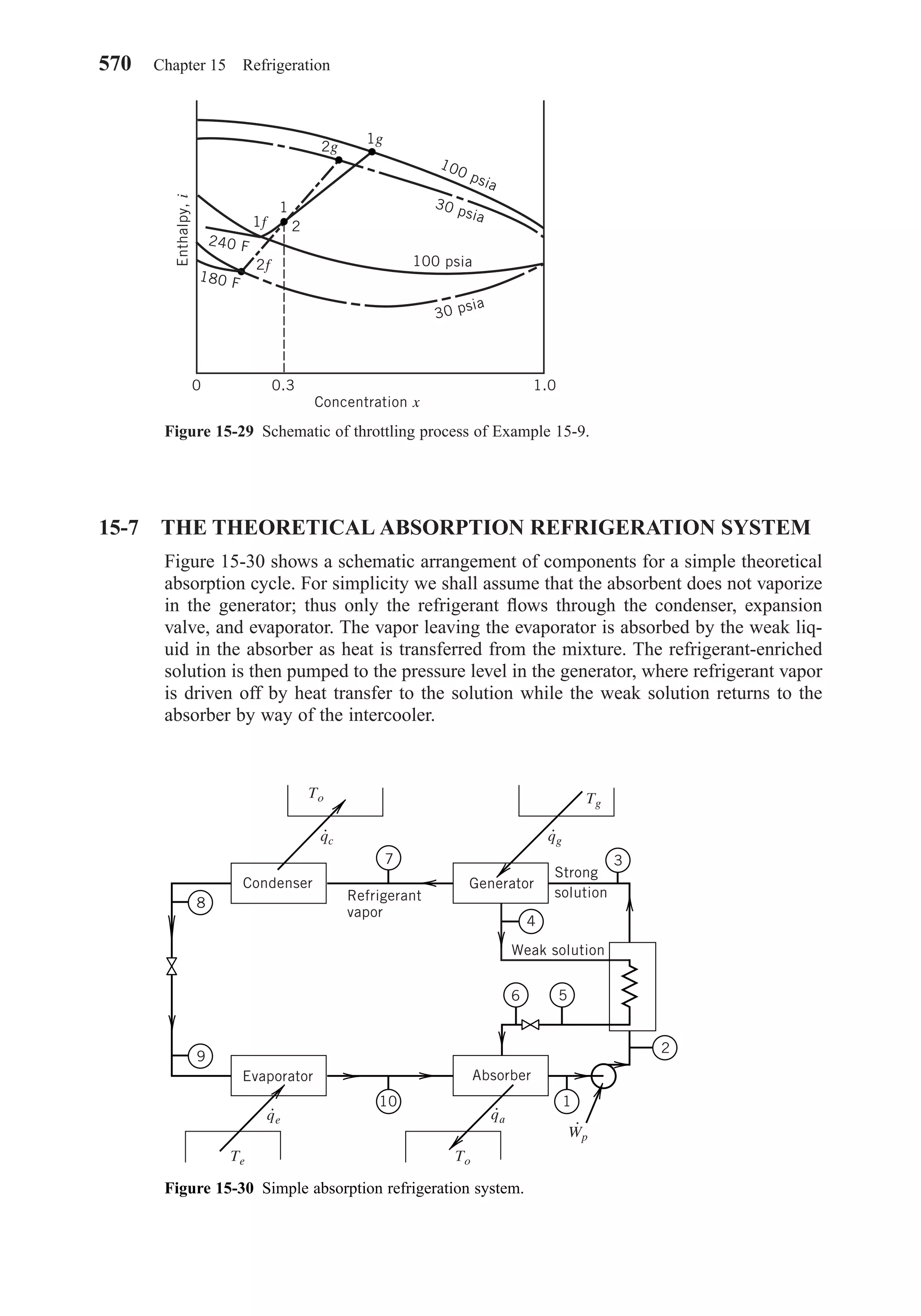
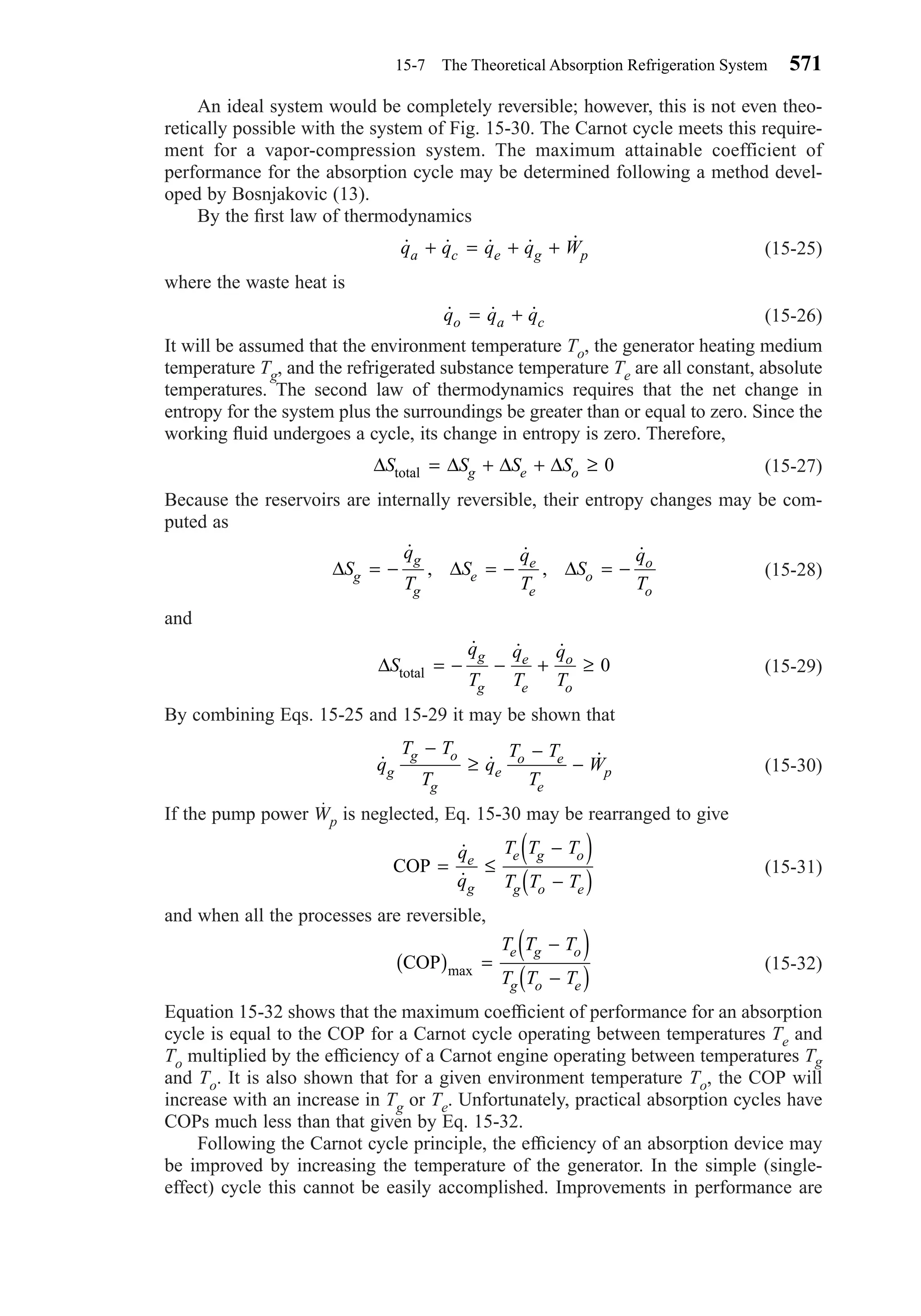
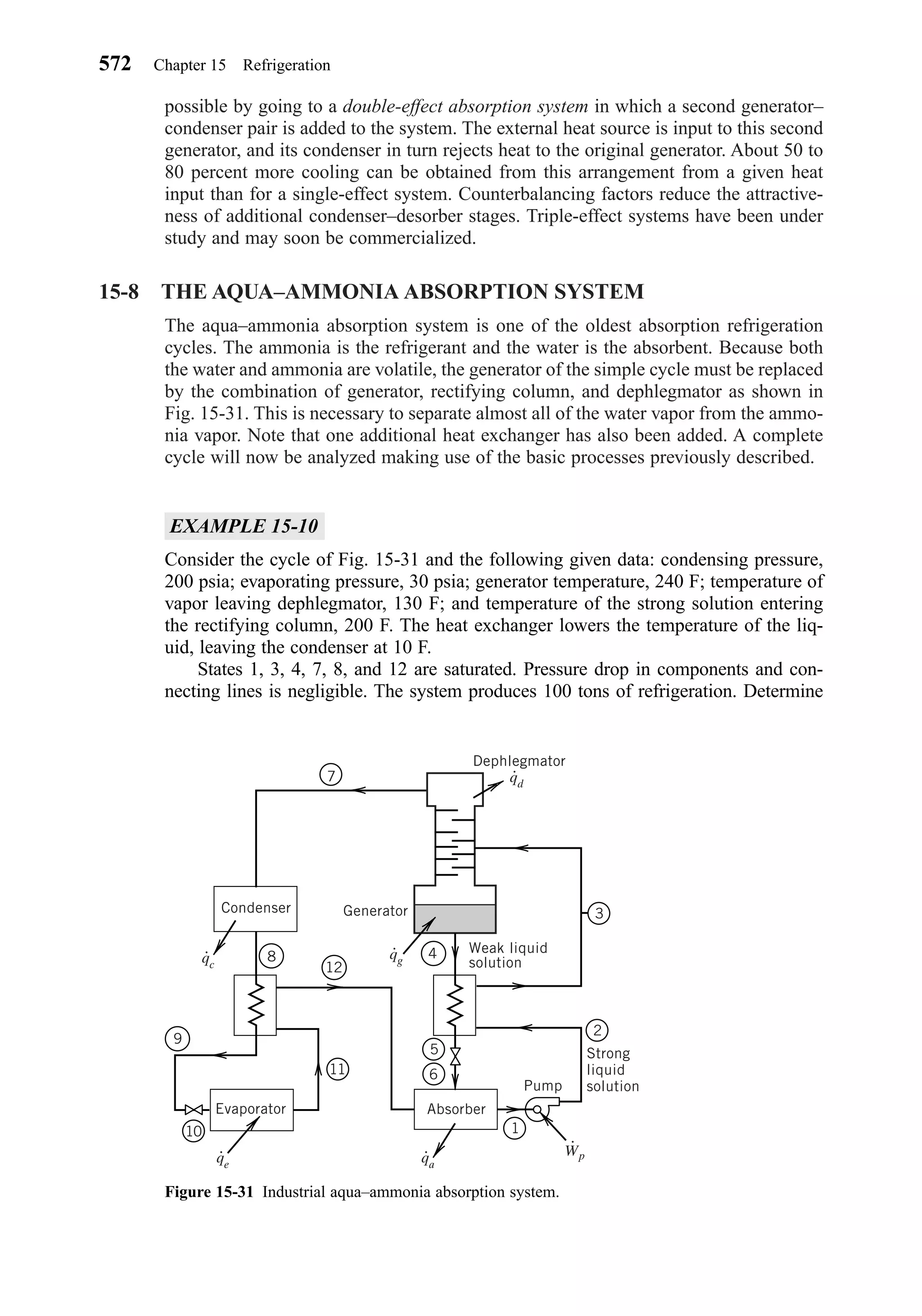
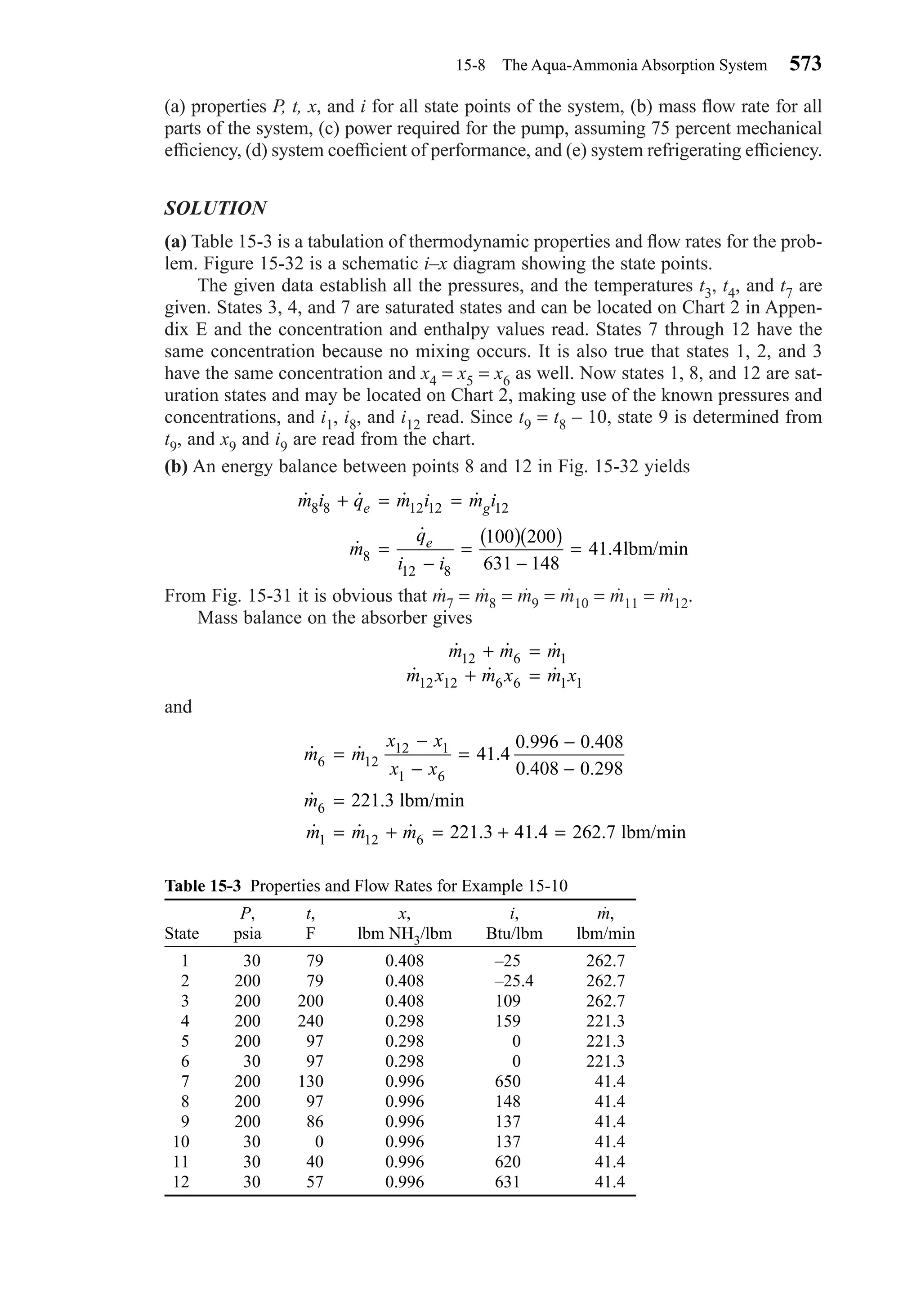
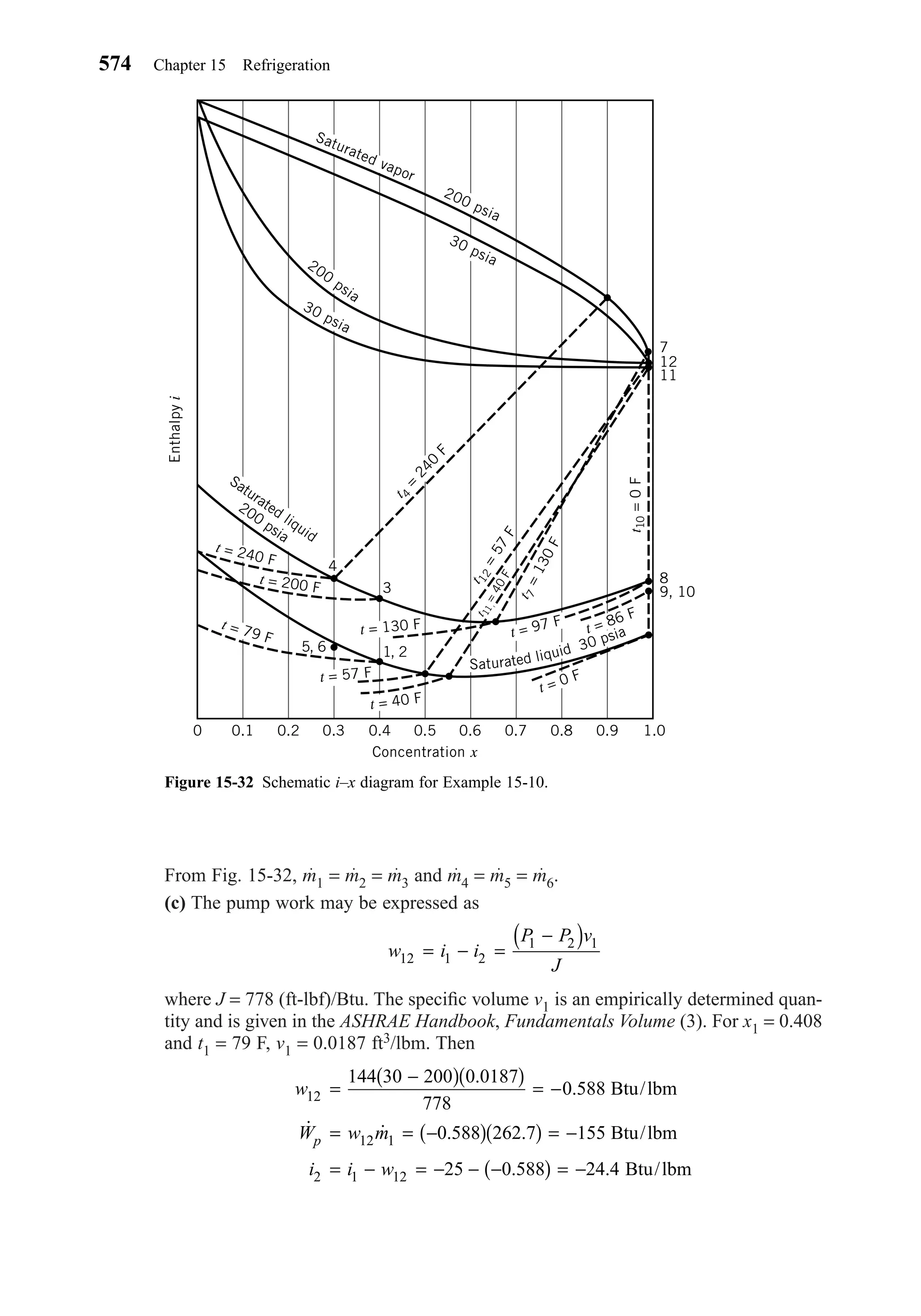
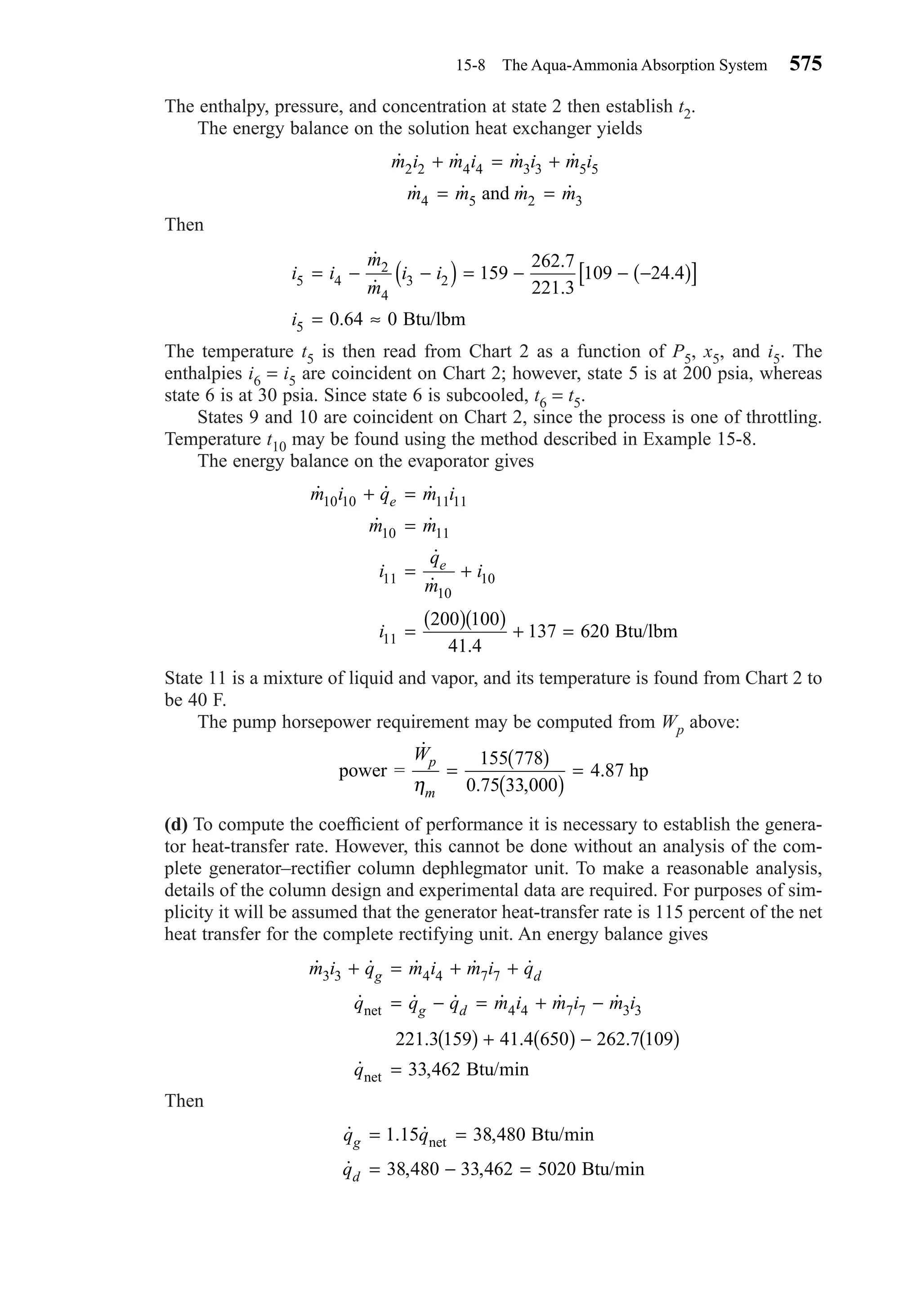
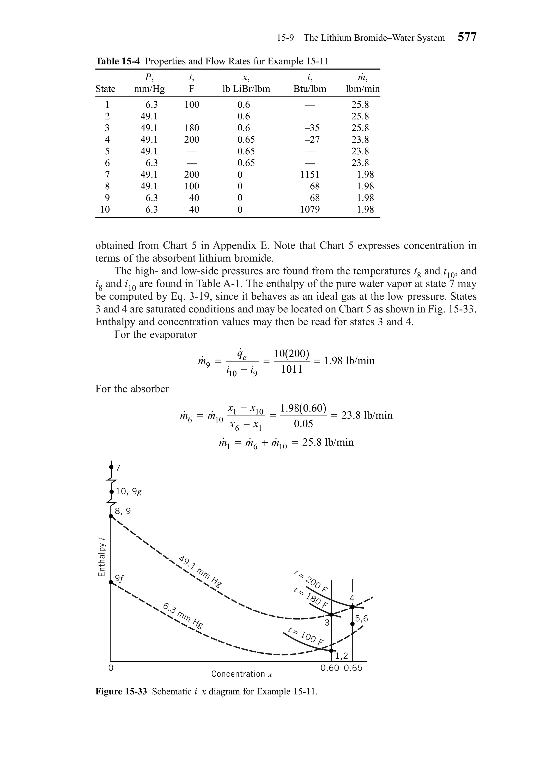
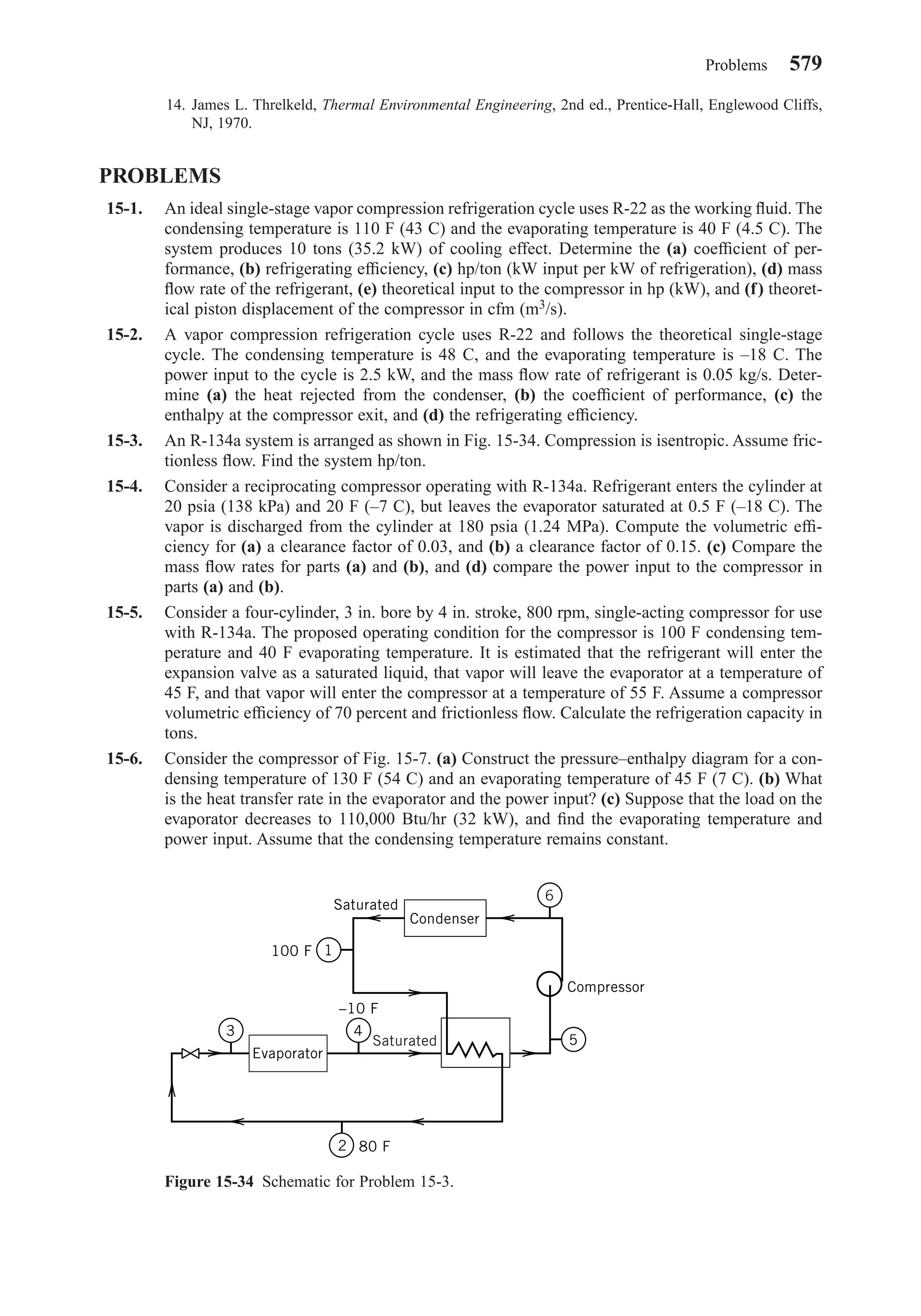
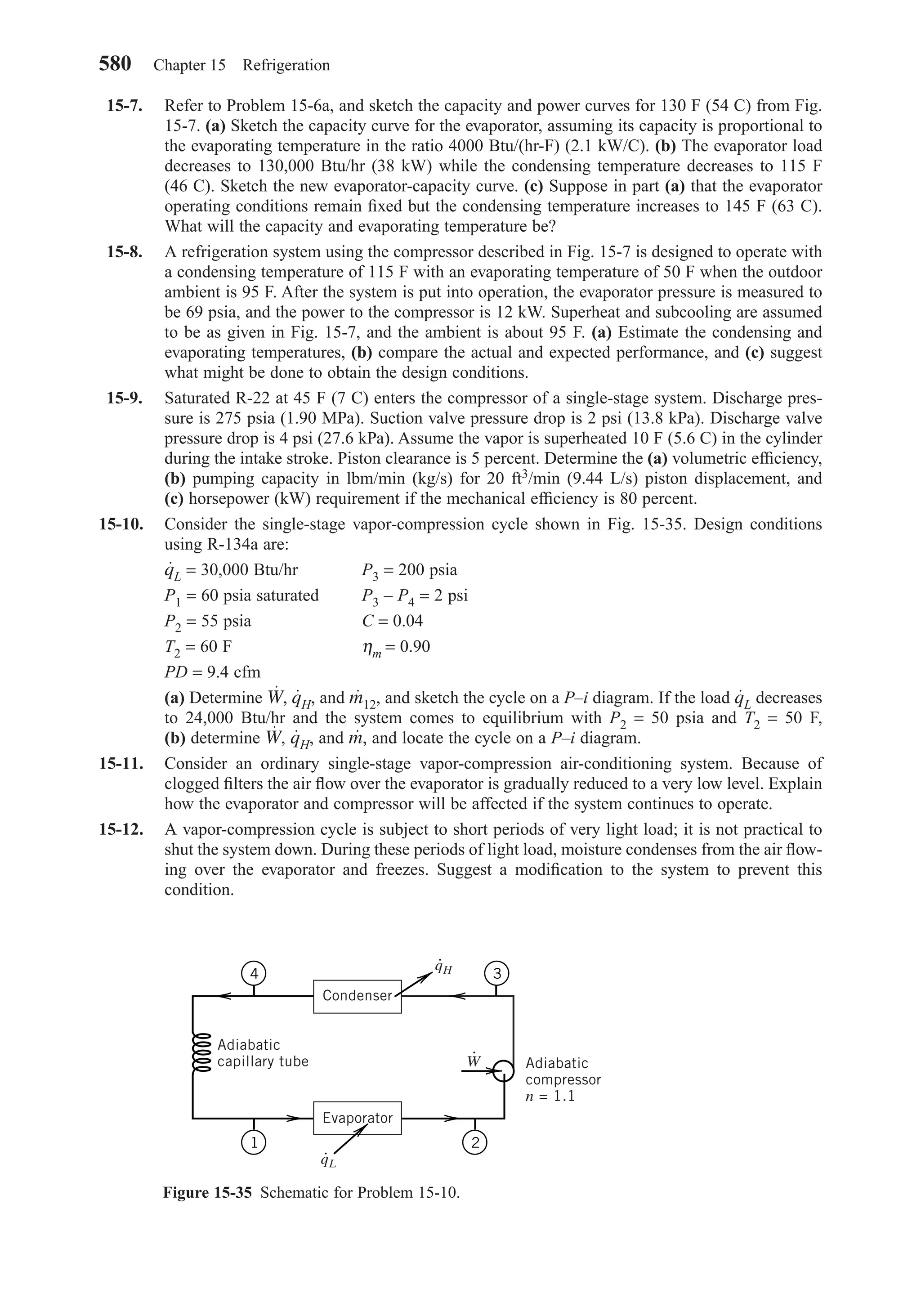

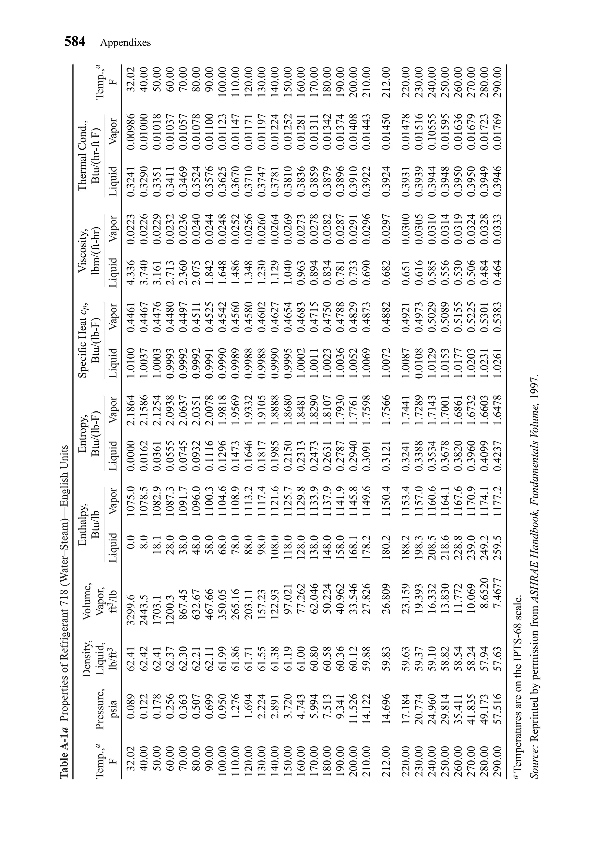
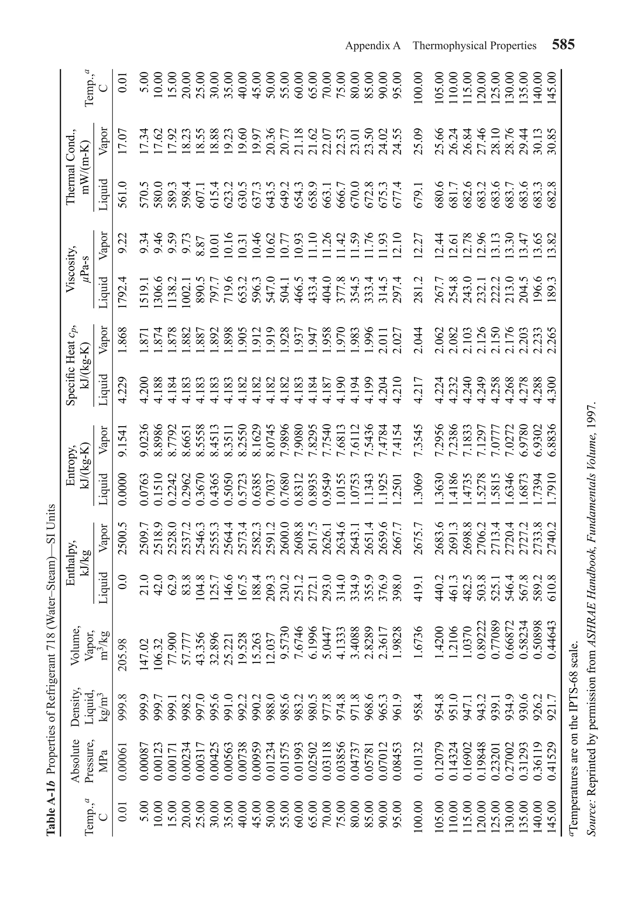
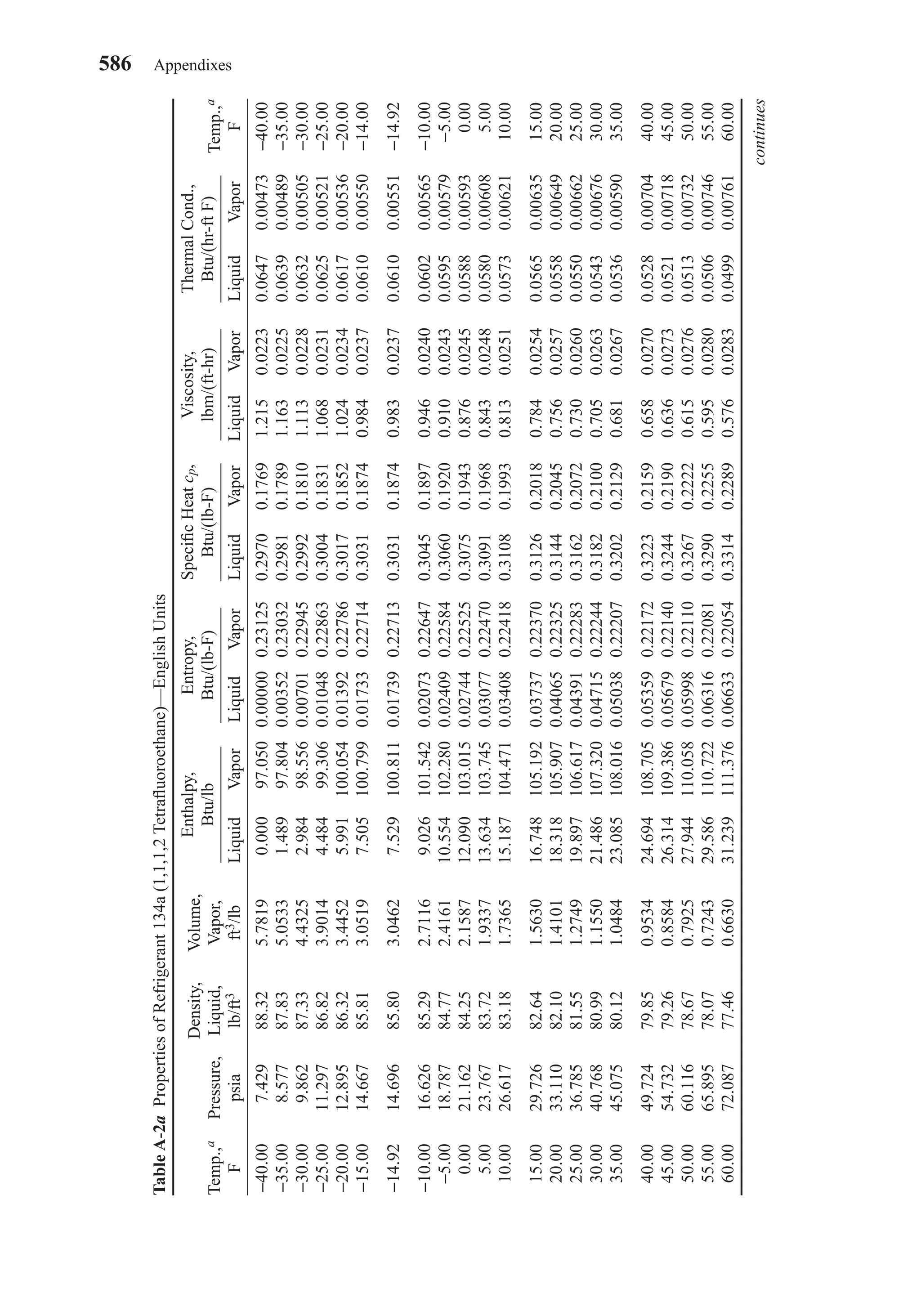

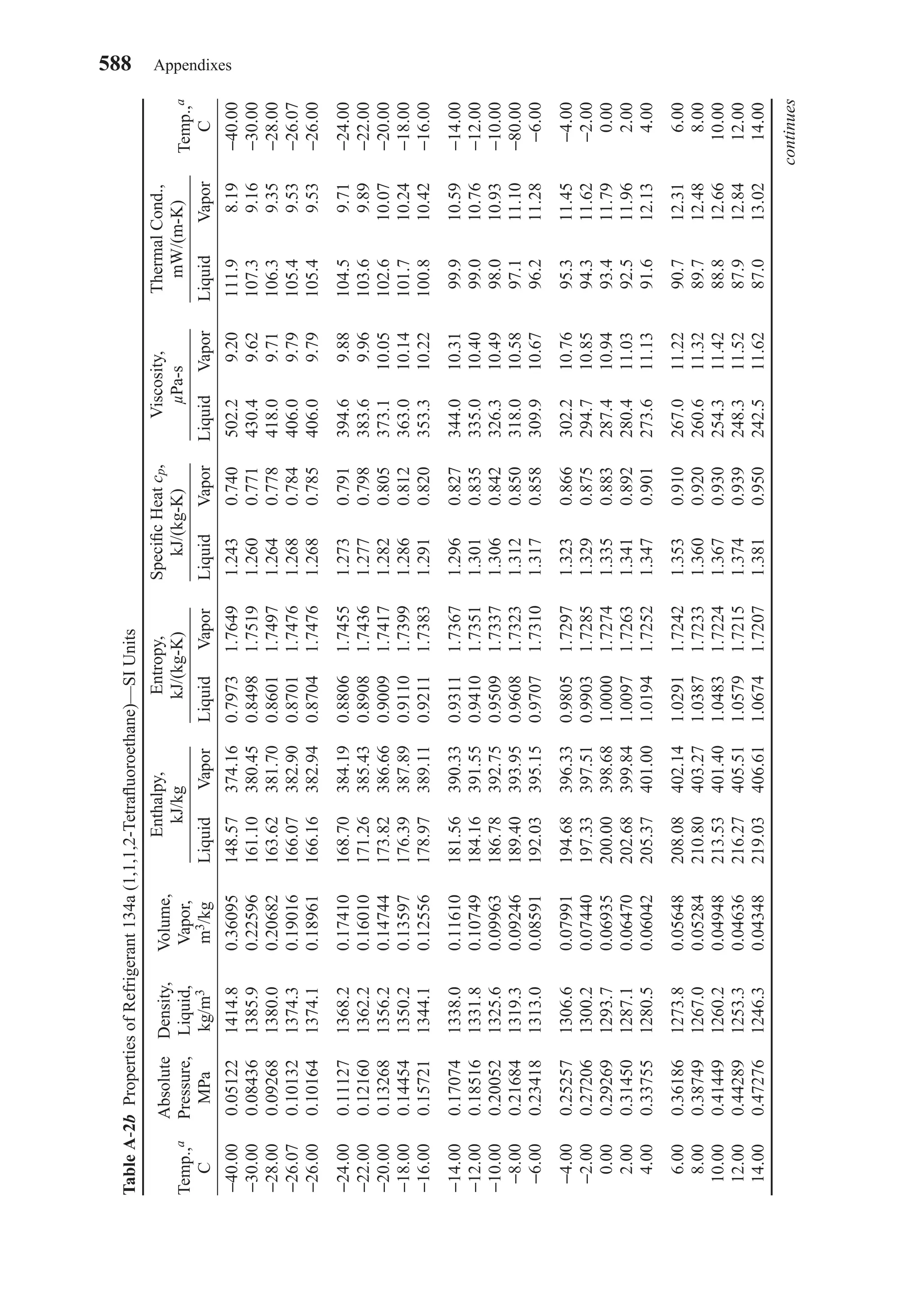
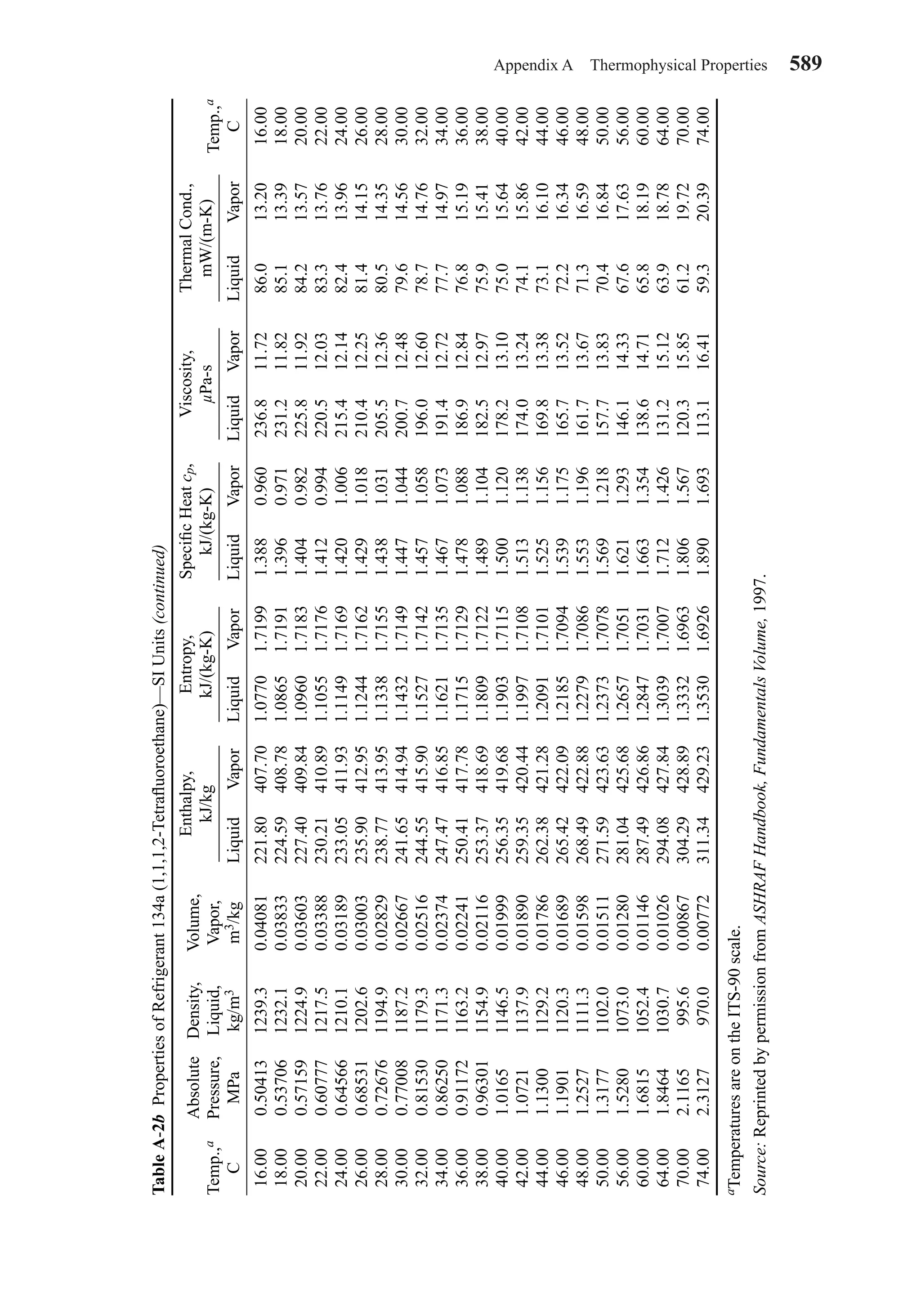
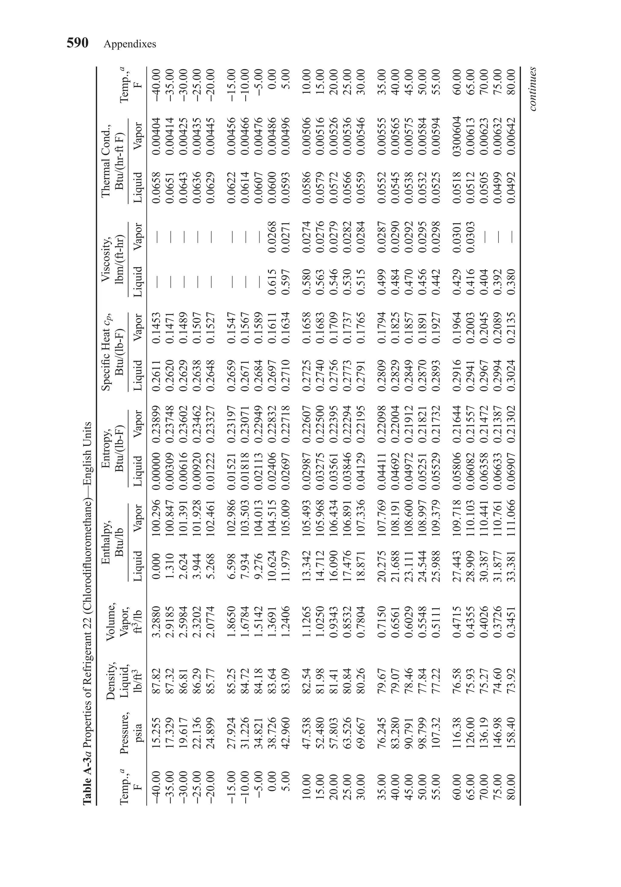
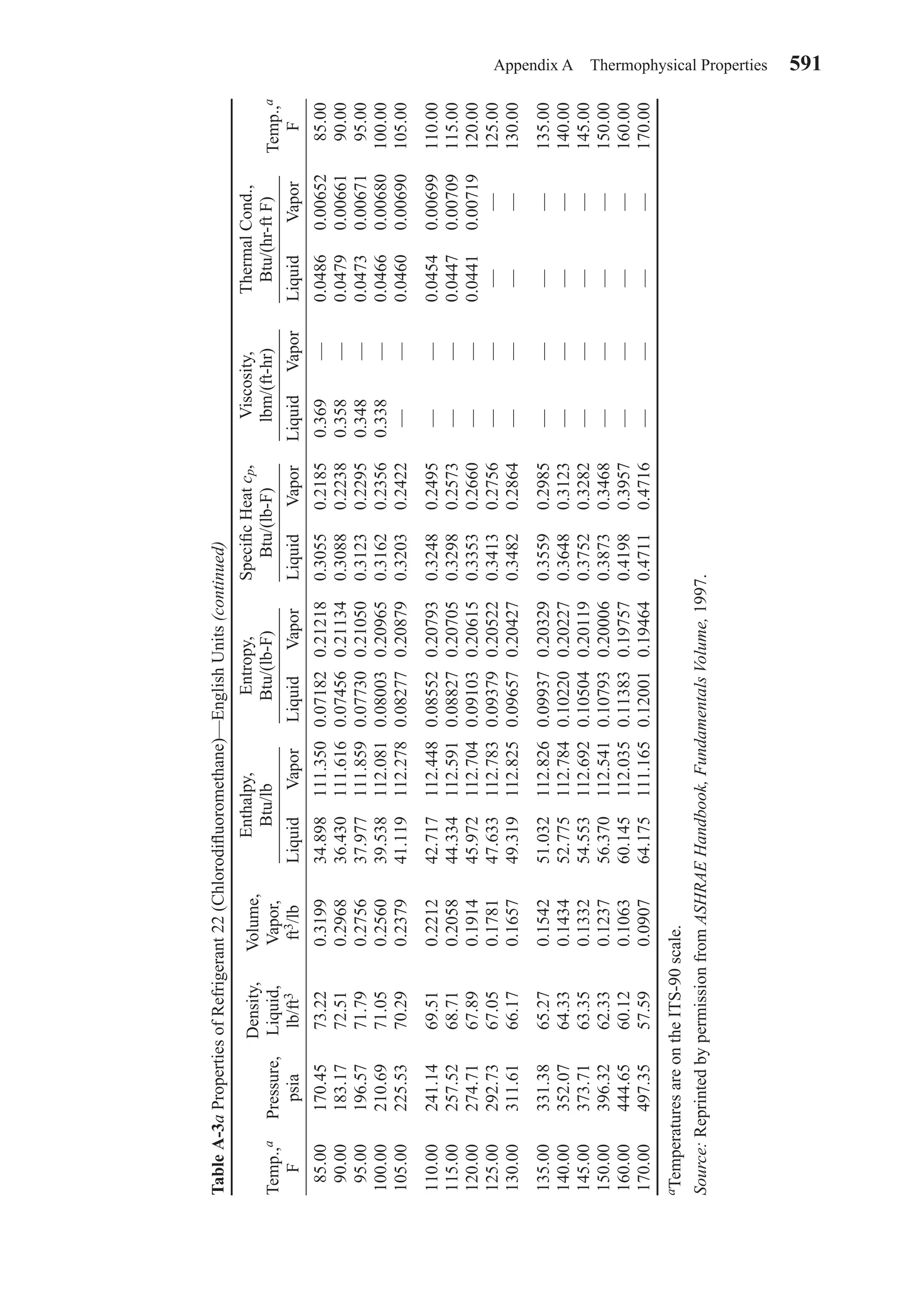
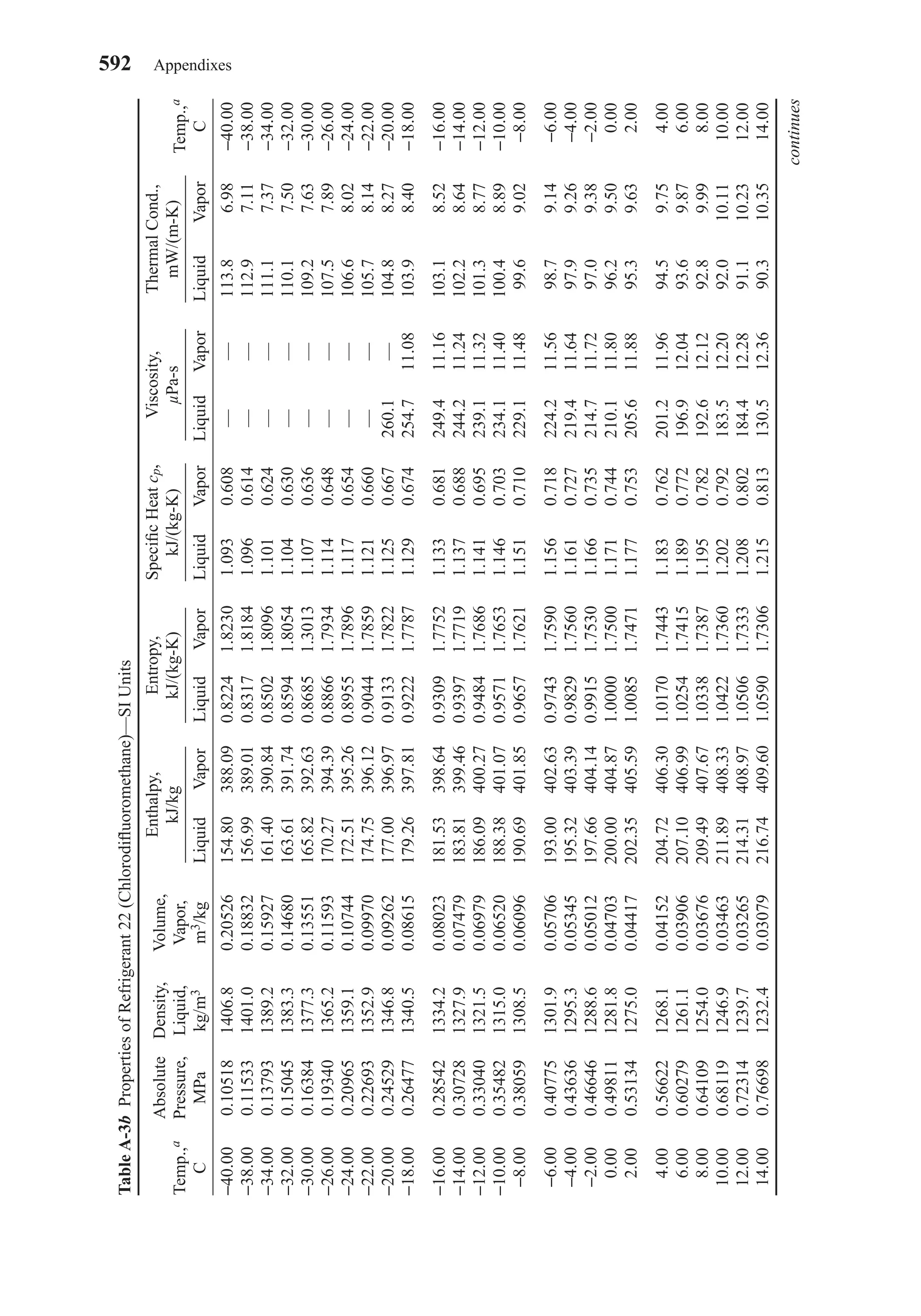
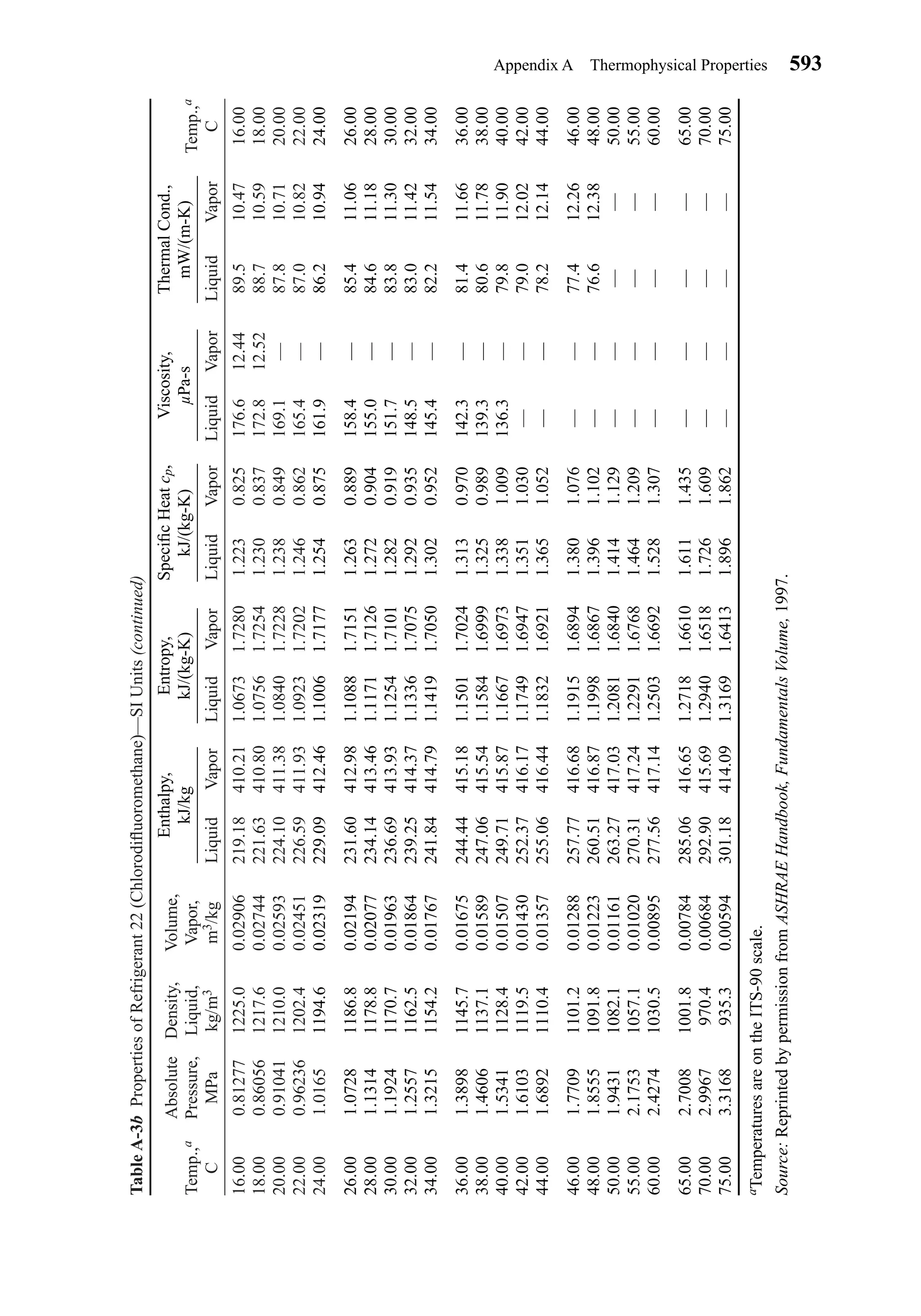
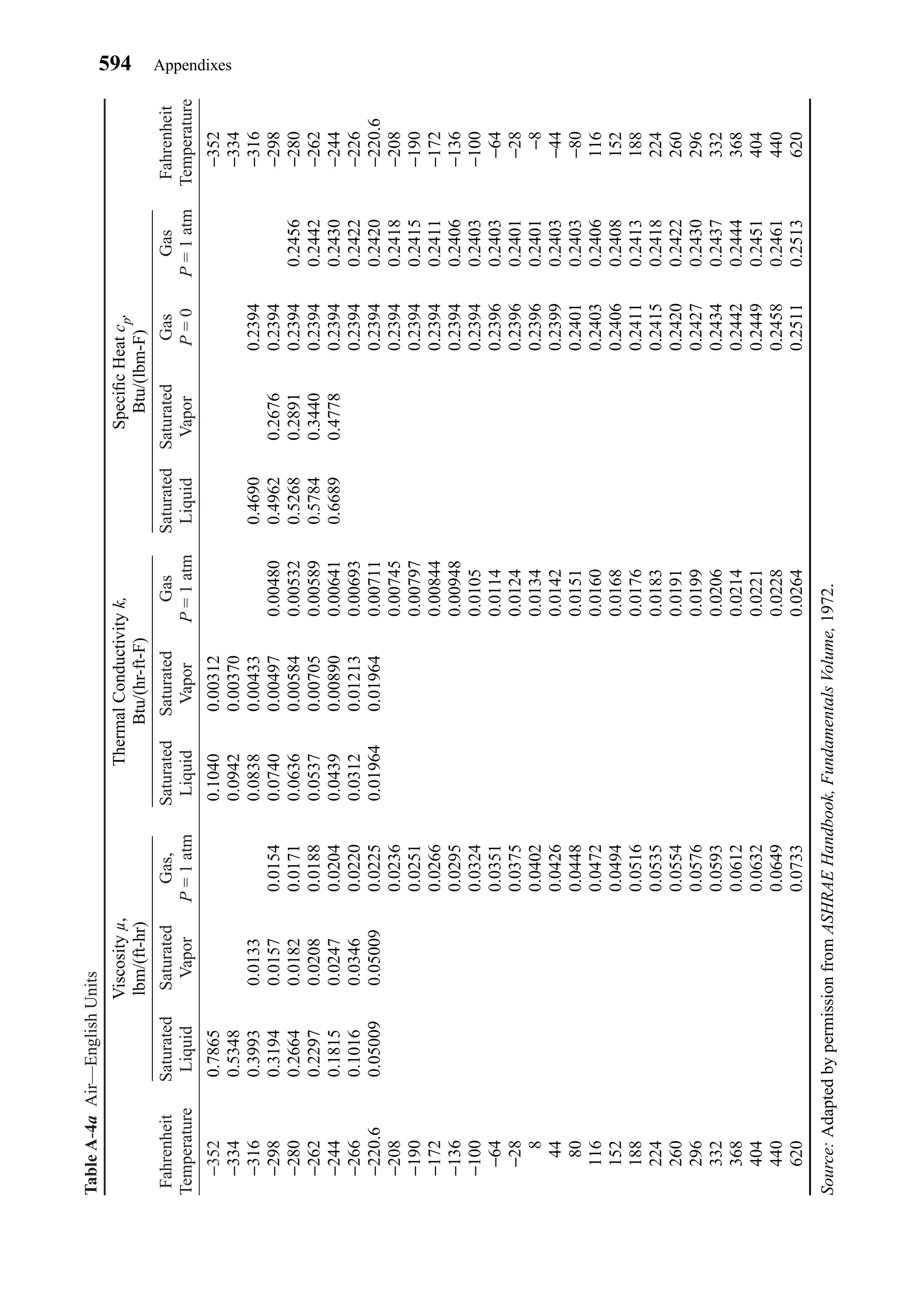
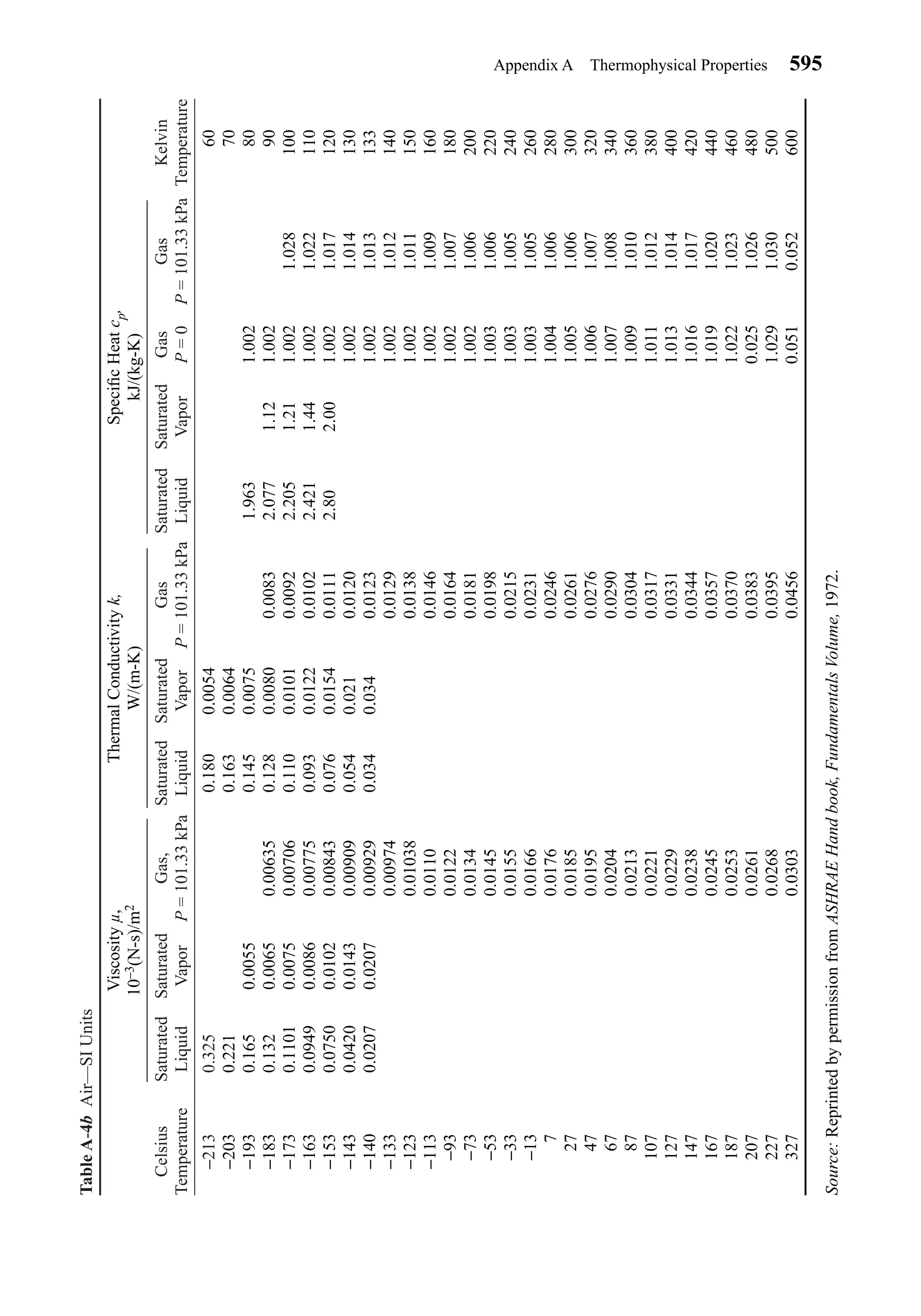
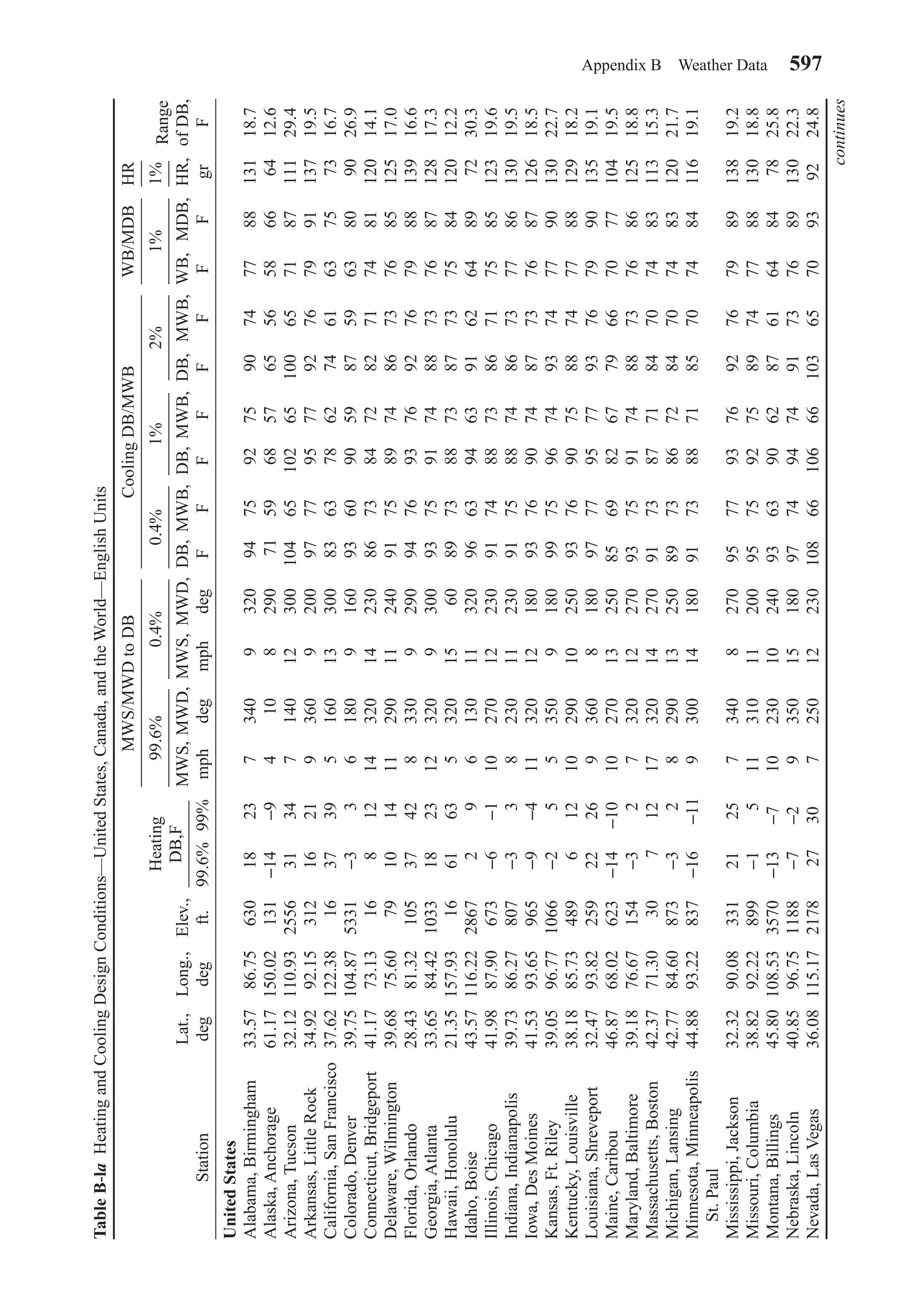
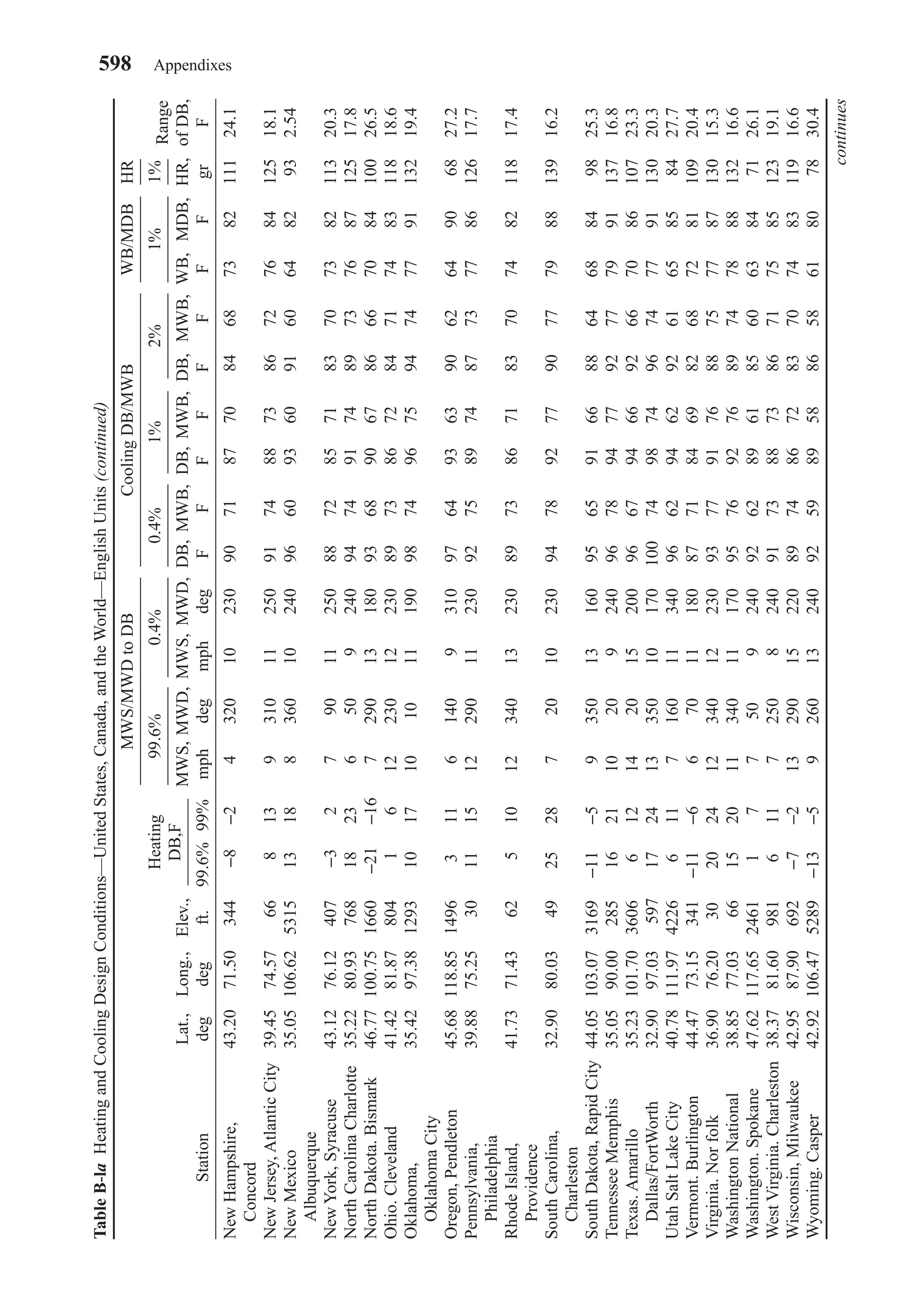
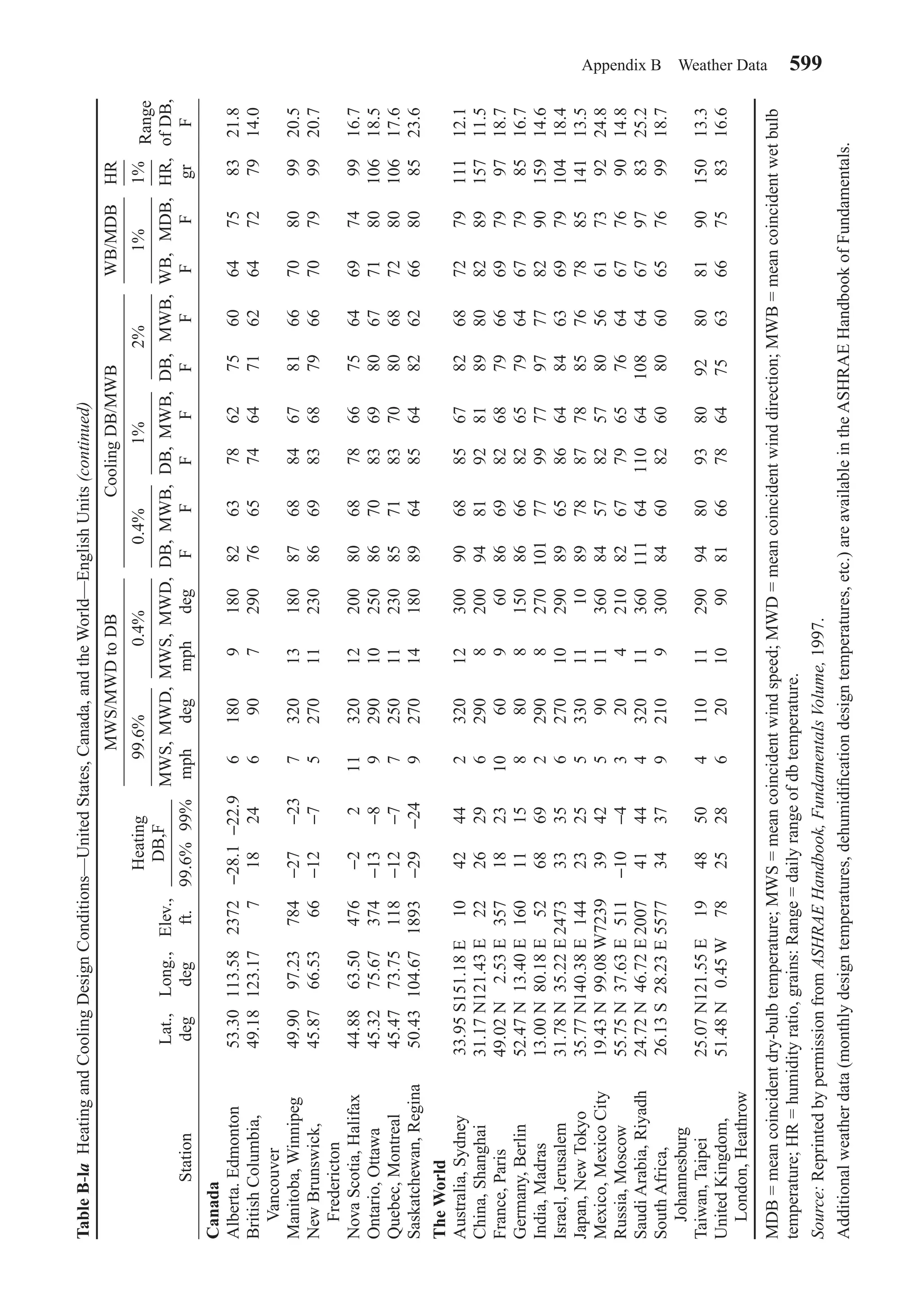
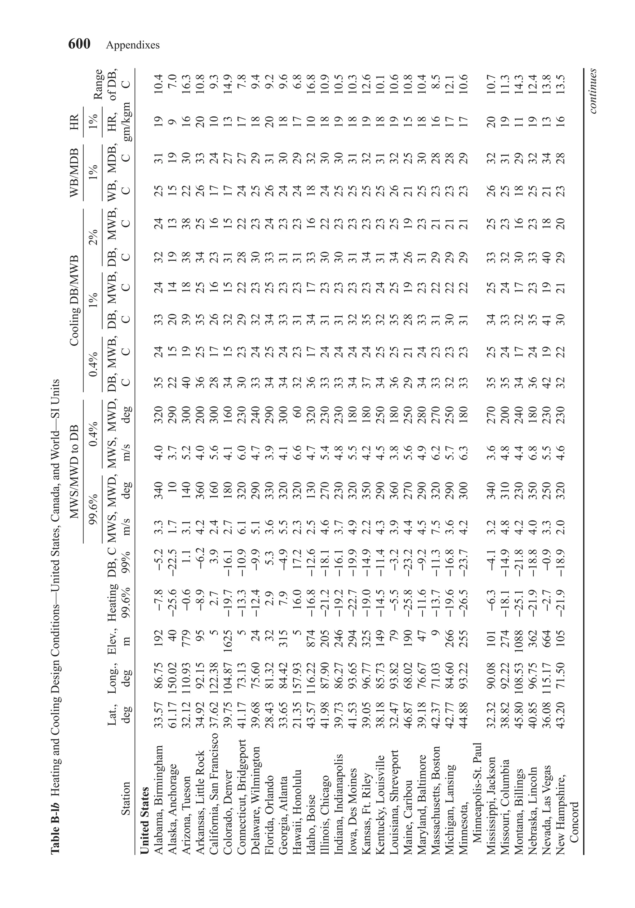
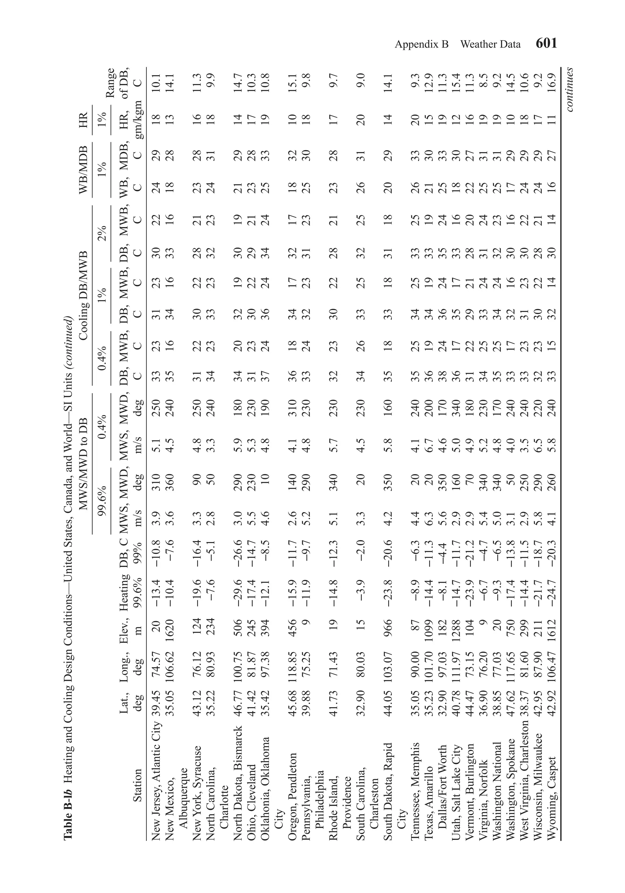
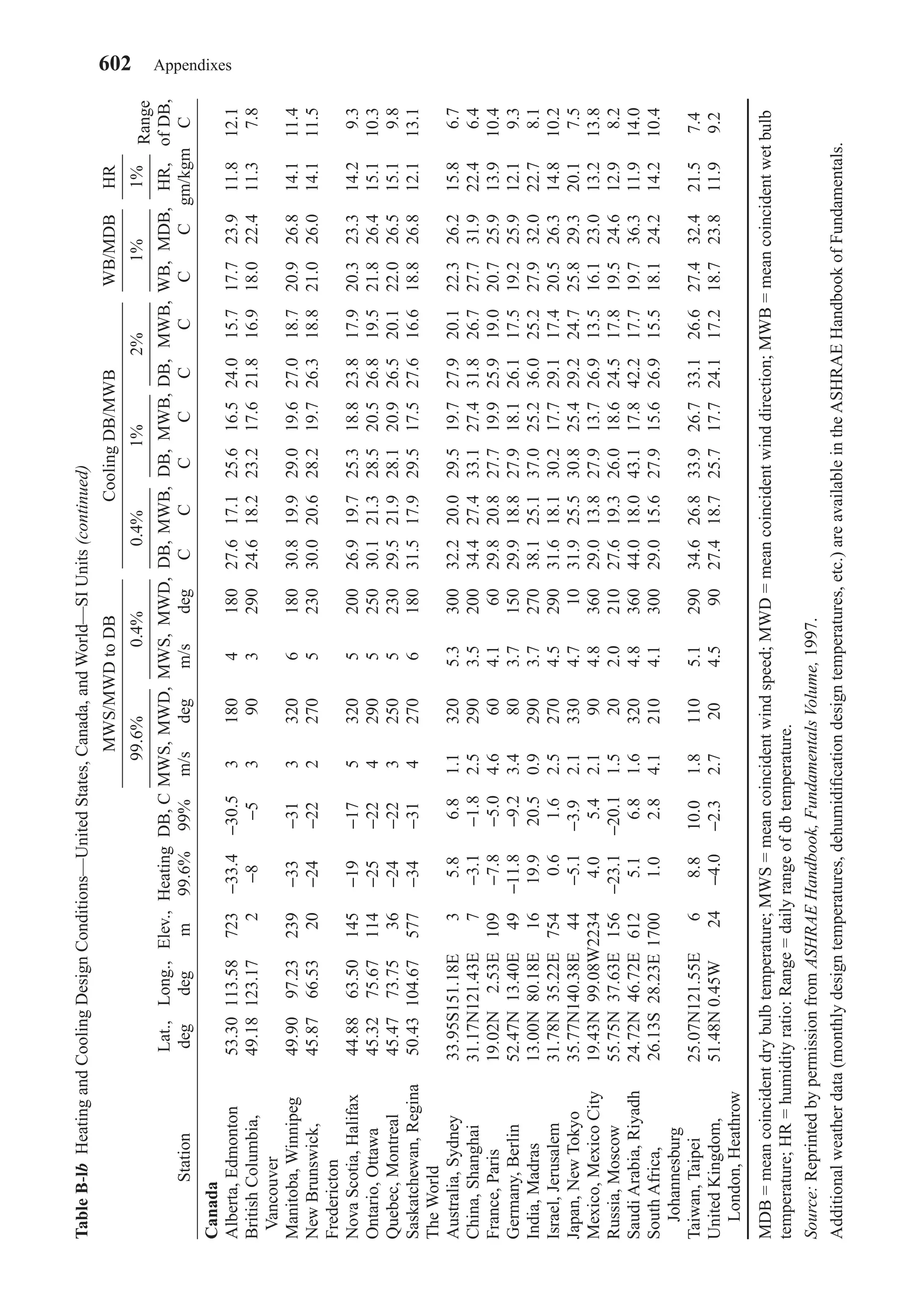
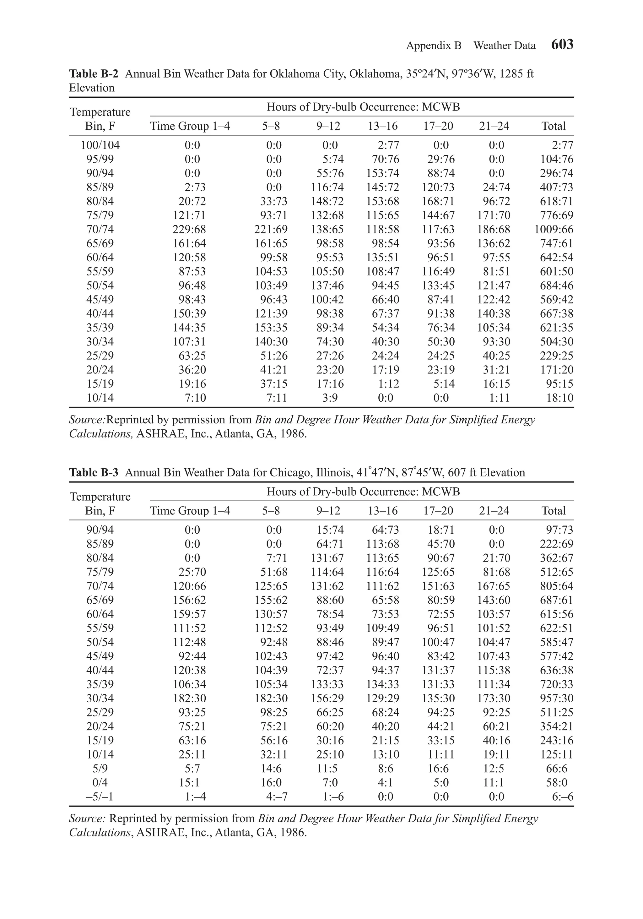
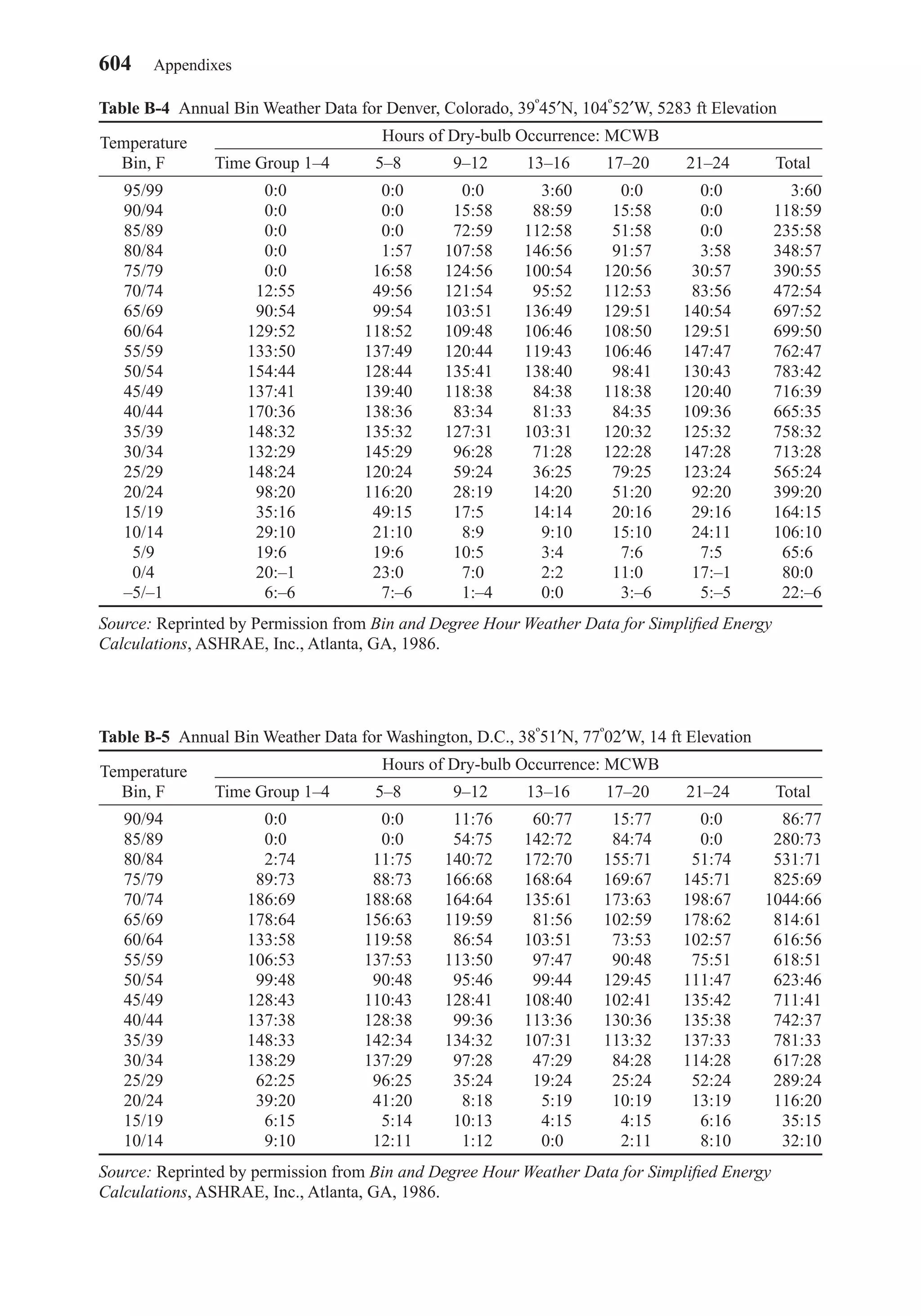
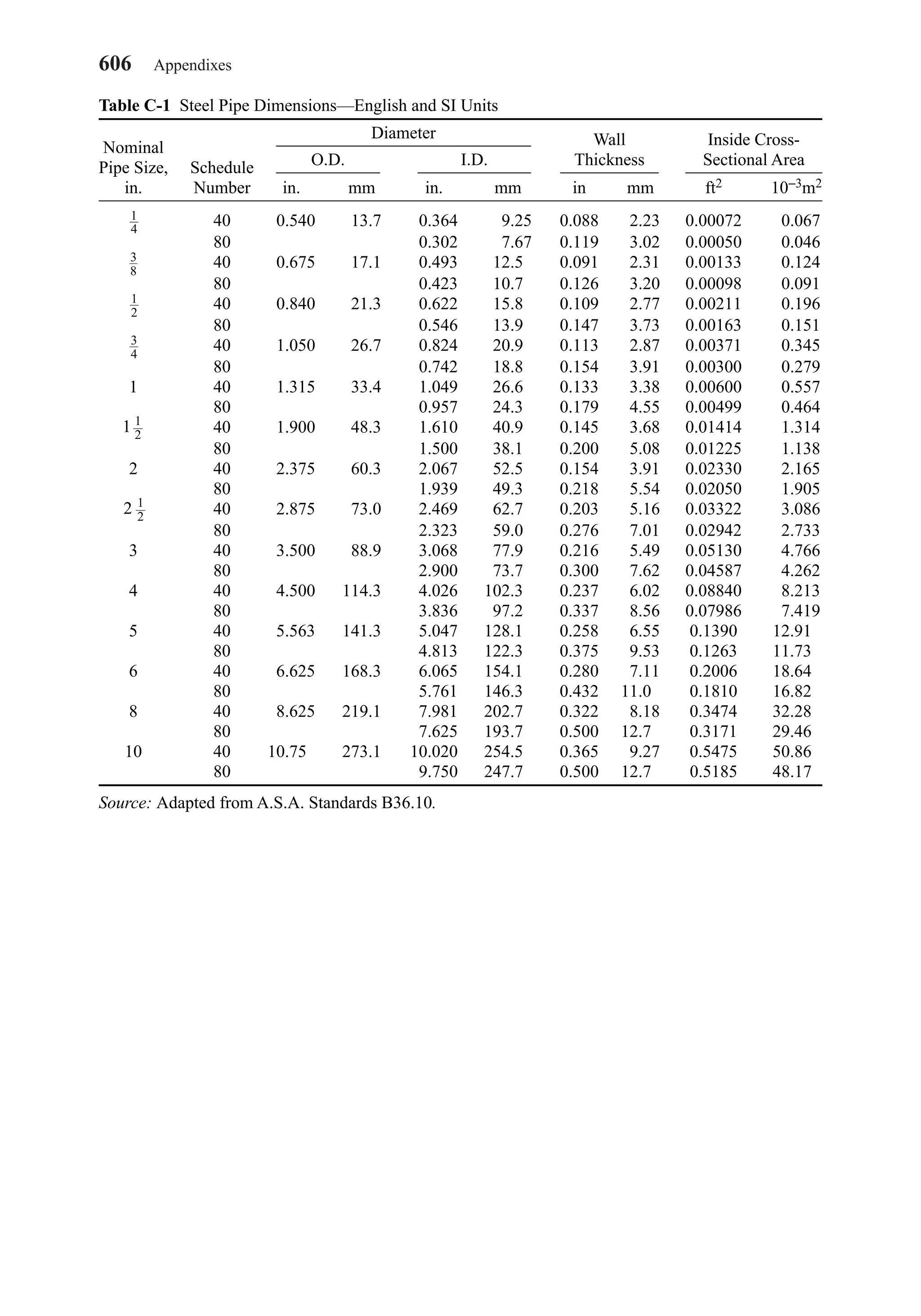
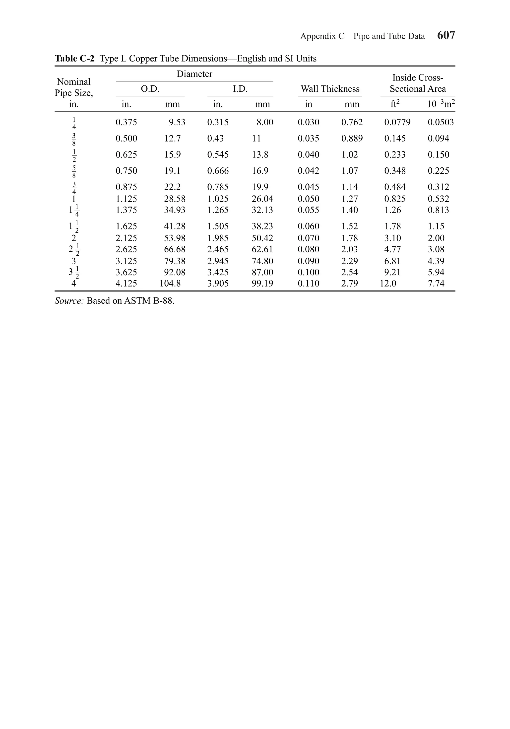

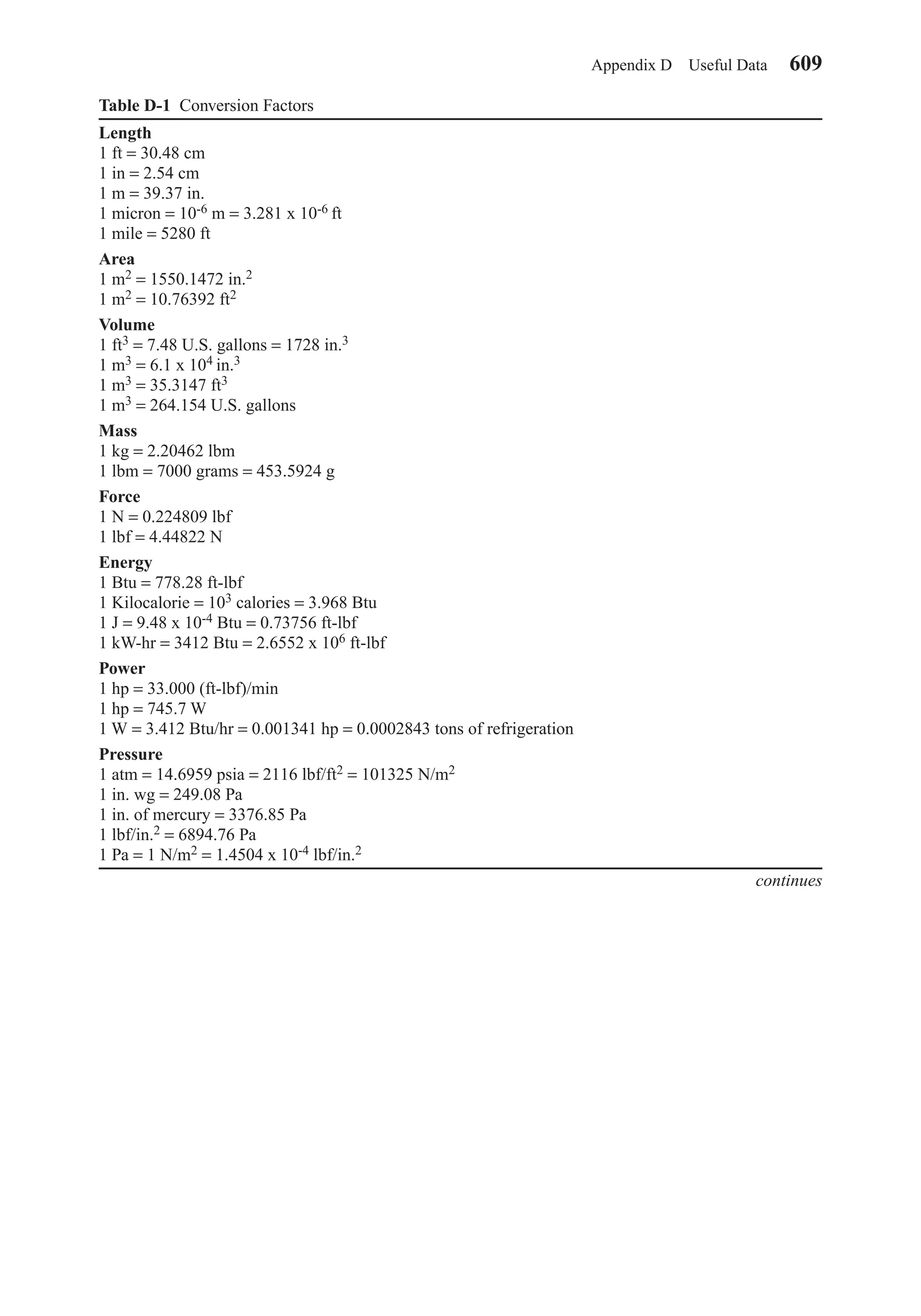
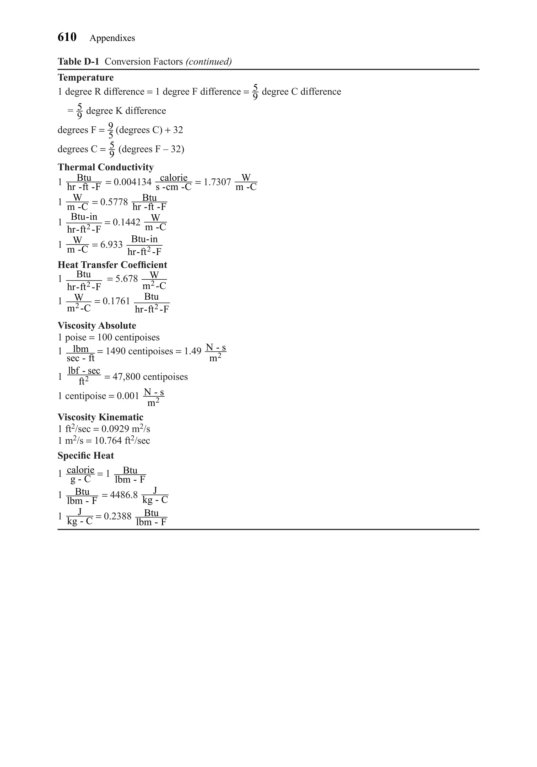
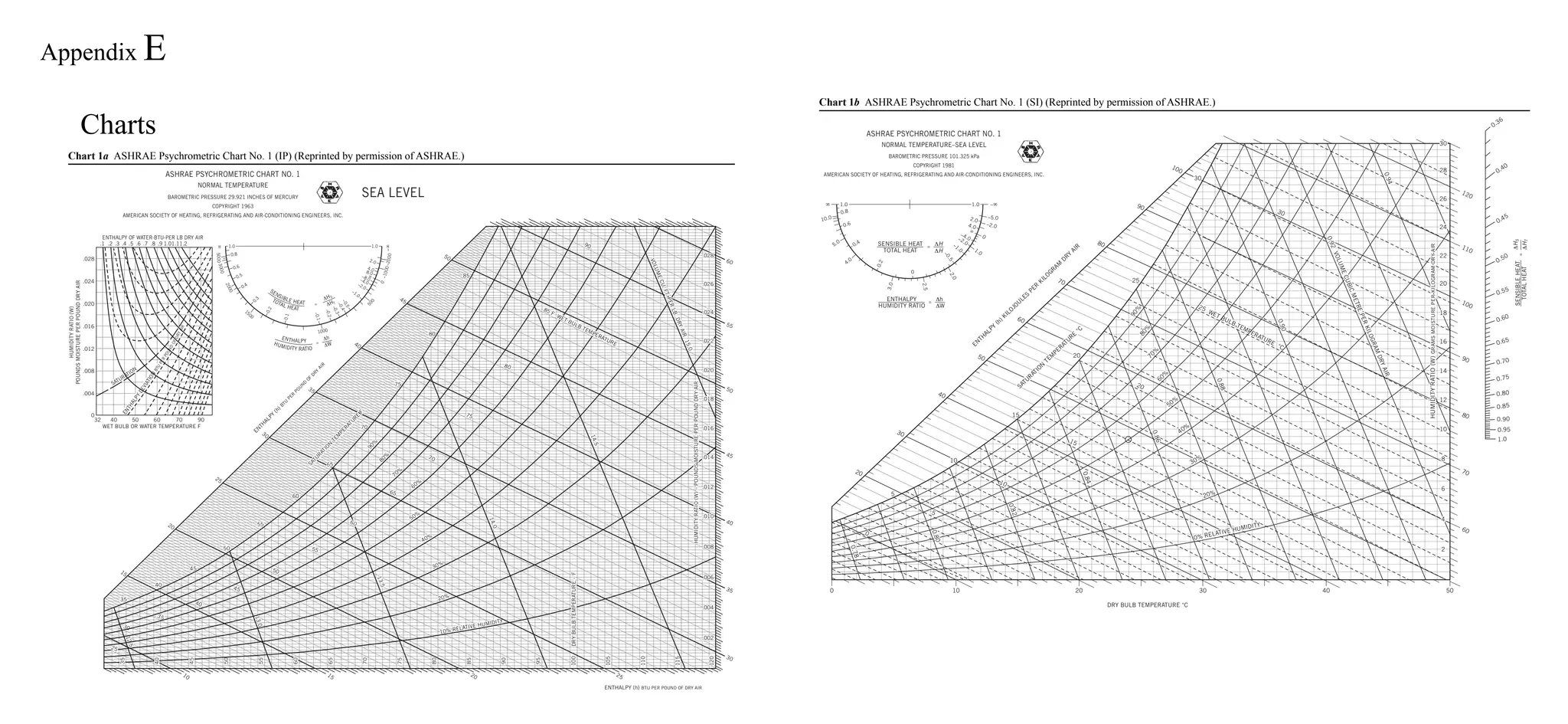
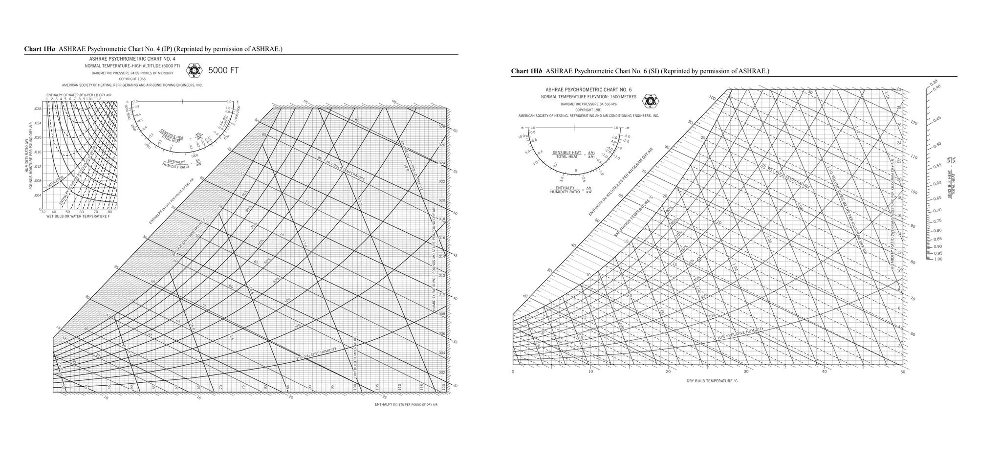

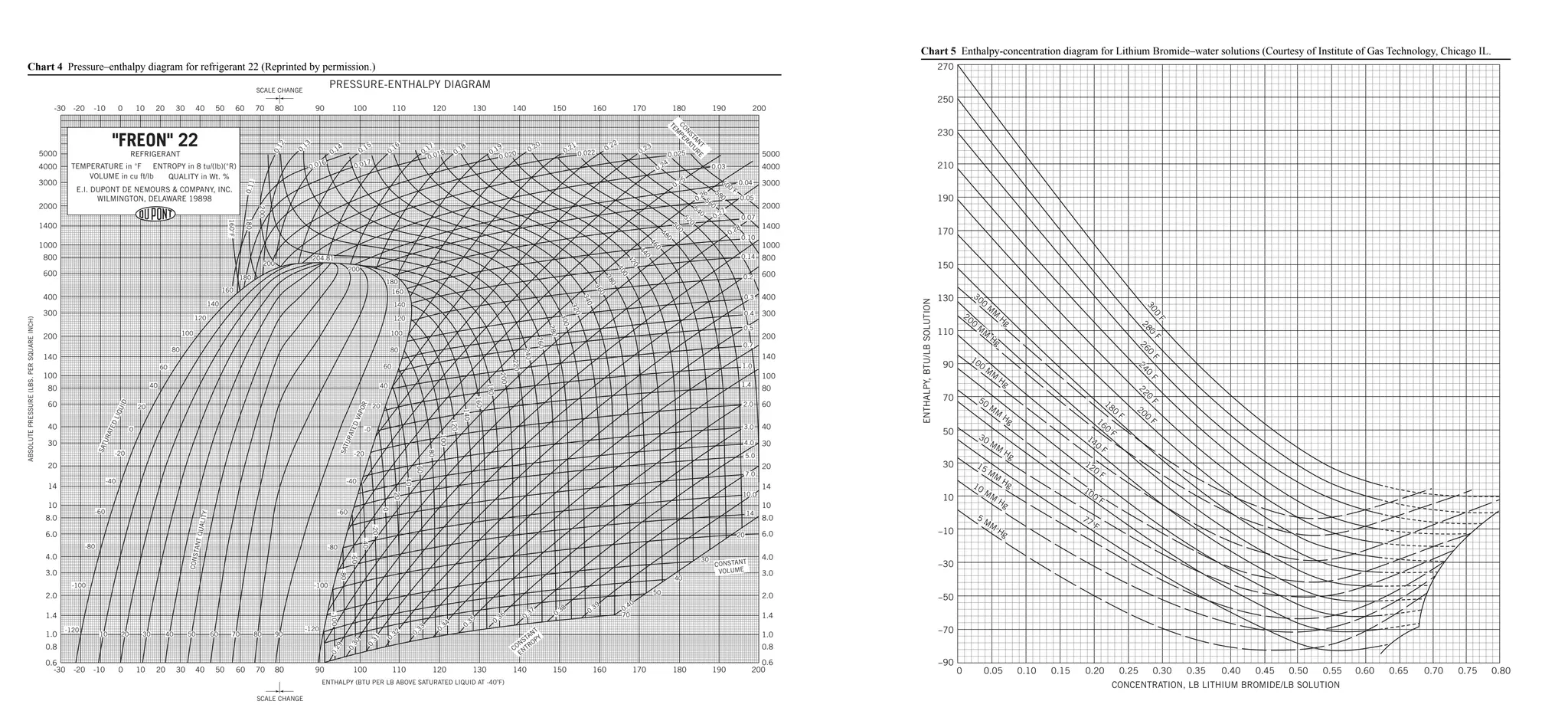
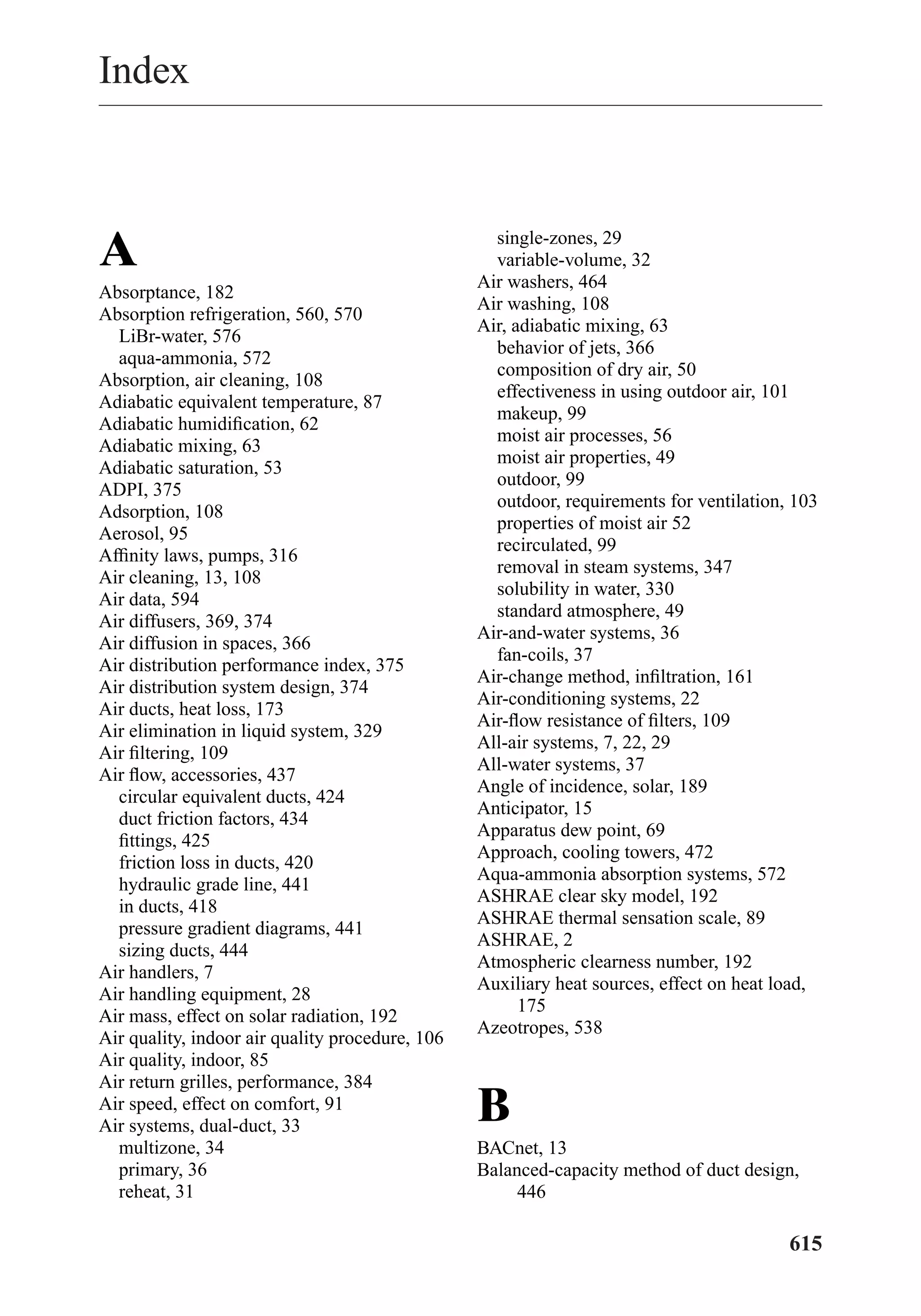

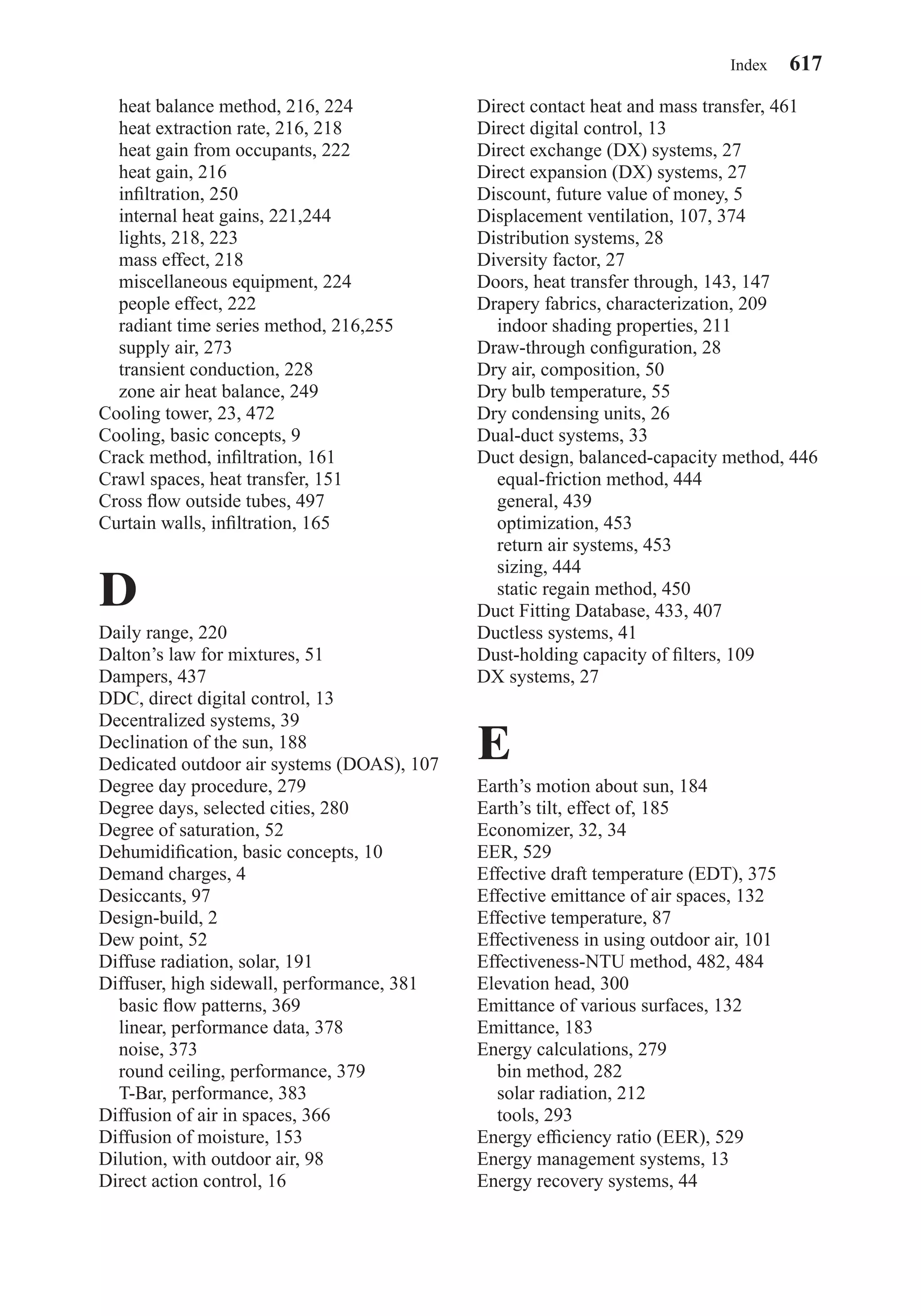
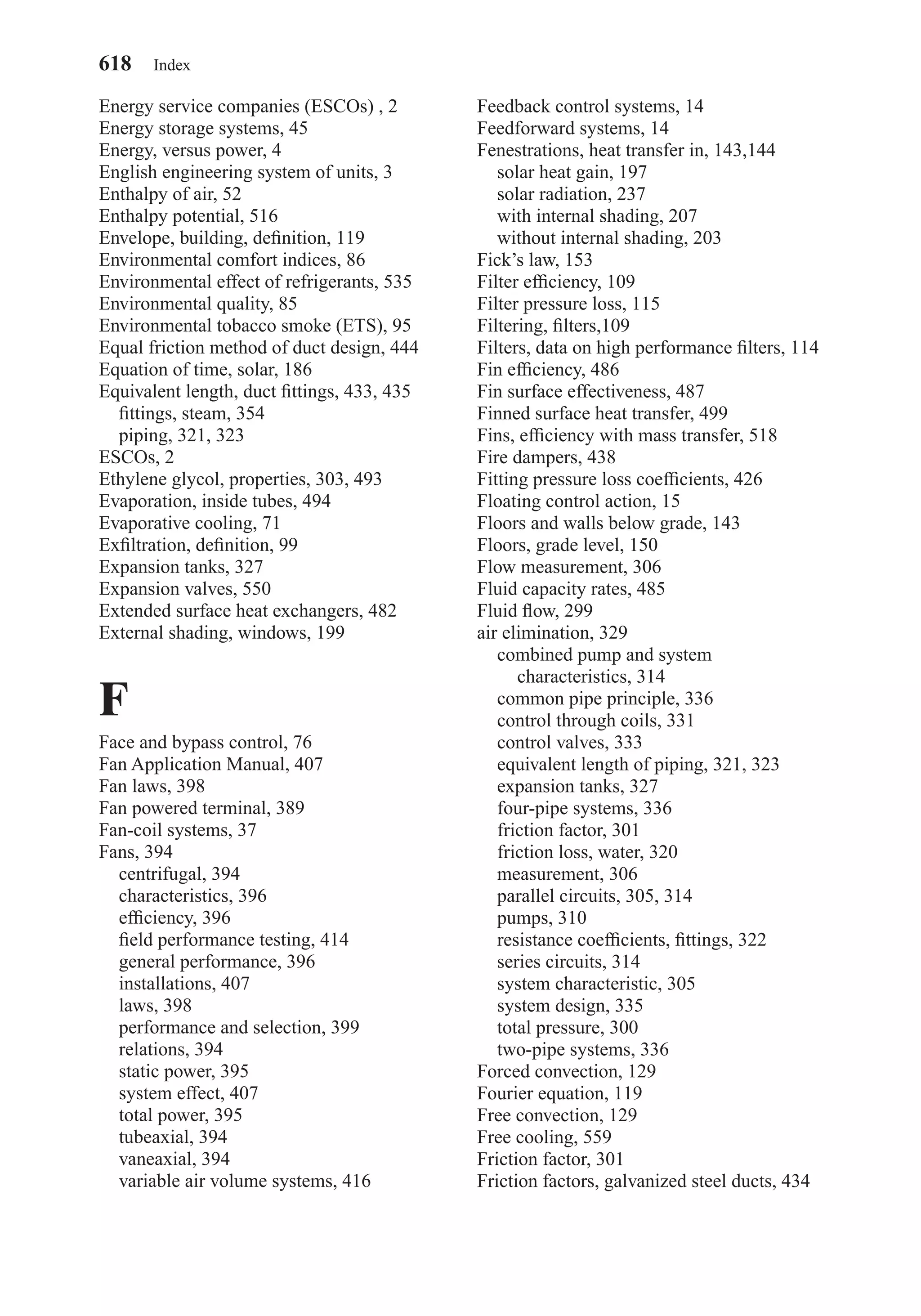
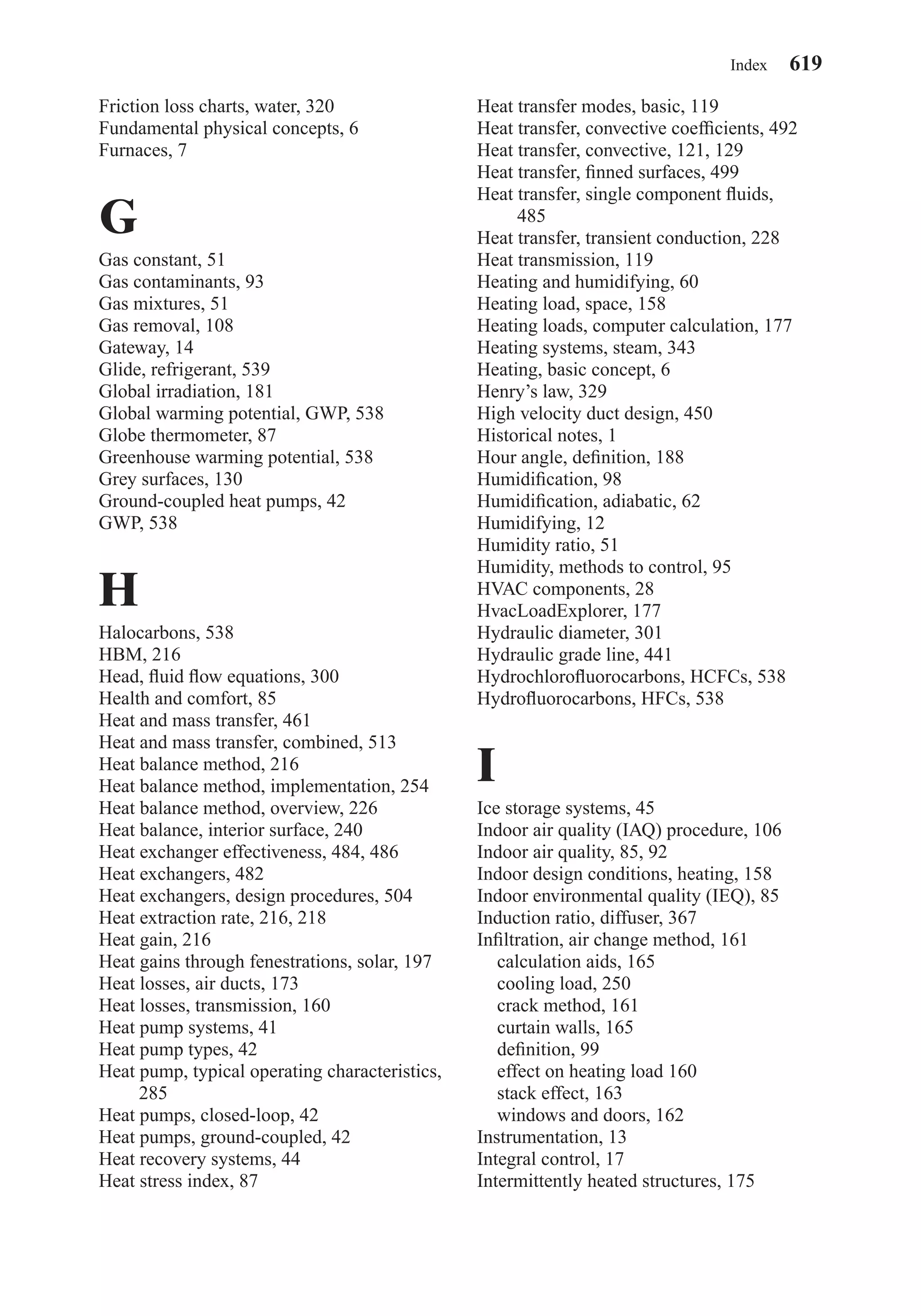
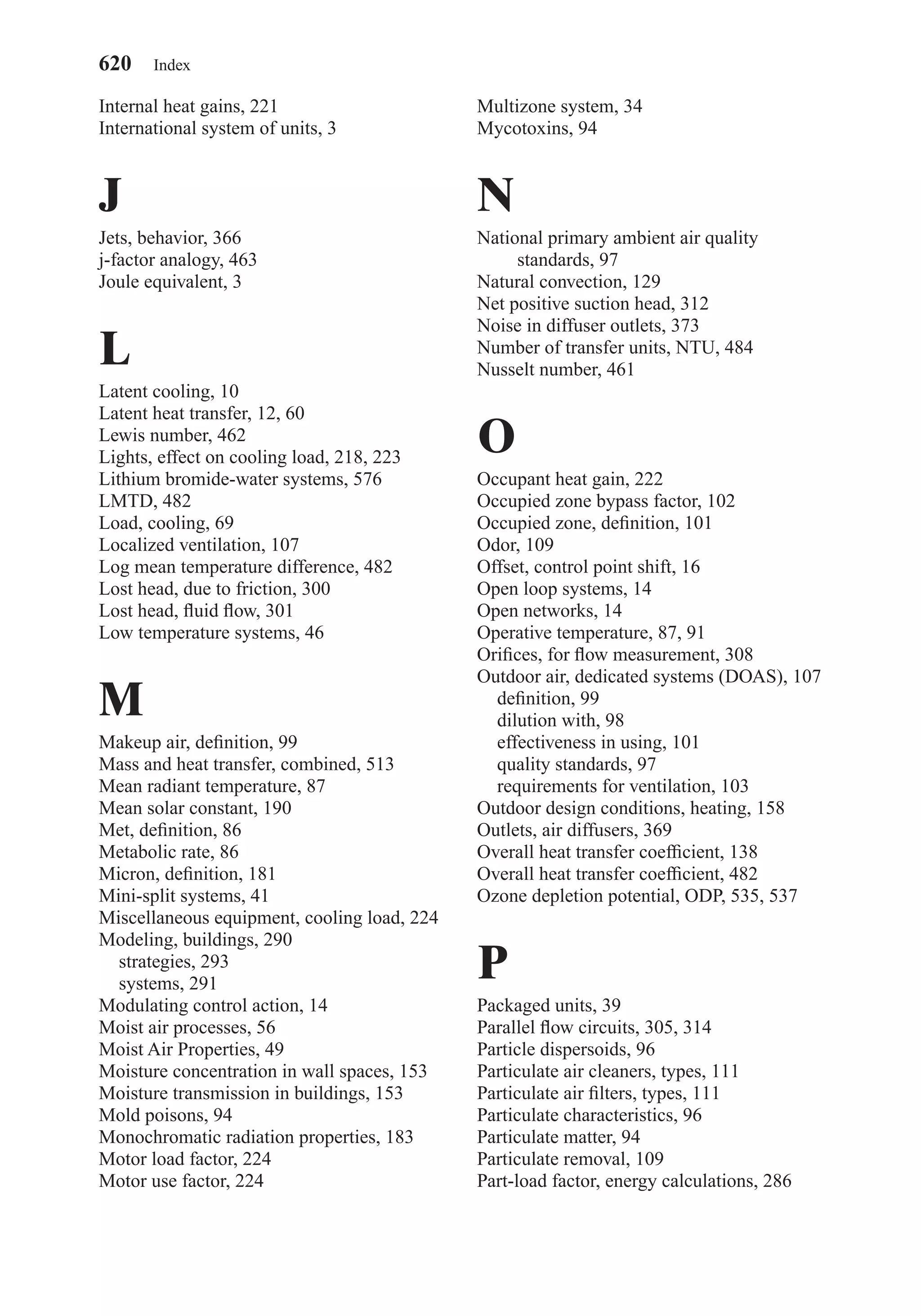

This document provides an overview of the 6th edition of the textbook "Heating, Ventilating, and Air Conditioning: Analysis and Design" by Faye C. McQuiston, Jerald D. Parker, and Jeffrey D. Spitler. The summary includes: 1) The textbook covers fundamental concepts of HVAC systems as well as analysis and design of air conditioning, heating, ventilation, and indoor air quality systems. 2) It provides an introduction to HVAC units and dimensions, moist air properties, comfort and indoor environmental quality, heat transfer in buildings, heating and cooling load calculations, energy calculations, fans and air distribution, and refrigeration systems. 3) The 6th


