Download to read offline
![Dr. Umakant Bhaskar Gohatre, Assistant Professor, SIGCE, Navi Mumbai, Mumbai University,
Maharashtra, India (This file for study purpose)
3
𝑦′(𝑡0) ≈
𝑦(𝑡0 + ℎ) − 𝑦(𝑡0)
ℎ
in the differential equation 𝑦′
= 𝑓(𝑡, 𝑦) Again, this yields the Euler method. A similar
computation leads to the midpoint method and the backward Euler method.
Finally, one can integrate the differential equation from 𝑡0 + ℎ and apply the fundamental
theorem of calculus to get
𝑦(𝑡0 + ℎ) − 𝑦(𝑡0) = ∫
𝑡0+ℎ
𝑡0
𝑓(𝑡, 𝑦(𝑡))d𝑡.
Now approximate the integral by the left-hand rectangle method
∫
𝑡0+ℎ
𝑡0
𝑓(𝑡, 𝑦(𝑡))d𝑡 ≈ ℎ𝑓(𝑡0, 𝑦(𝑡0)).
Local truncation error
The local truncation error of the Euler method is the error made in a single step
𝑦1 = 𝑦0 + ℎ𝑓(𝑡0, 𝑦0).
For the exact solution, we use the Taylor expansion mentioned in the section Derivation above
𝑦(𝑡0 + ℎ) = 𝑦(𝑡0) + ℎ𝑦′(𝑡0) +
1
2
ℎ2
𝑦″(𝑡0) + 𝑂(ℎ3).
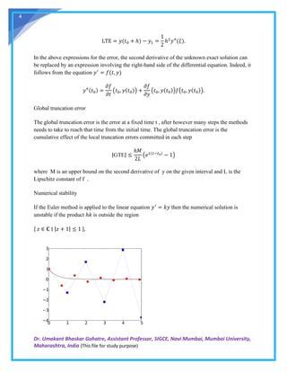
The local truncation error (LTE) introduced by the Euler method is given by the difference
between these equations
LTE = 𝑦(𝑡0 + ℎ) − 𝑦1 =
1
2
ℎ2
𝑦″(𝑡0) + 𝑂(ℎ3).
A slightly different formulation for the local truncation error can be obtained by using the
Lagrange form for the remainder term in Taylor's theorem
If 𝑦 has a continuous second derivative, then there exists a 𝜉 ∈ [𝑡0, 𝑡0 + ℎ] such that](https://image.slidesharecdn.com/eulermethoddetails-220809105254-853a9e97/85/Euler-Method-Details-3-320.jpg)

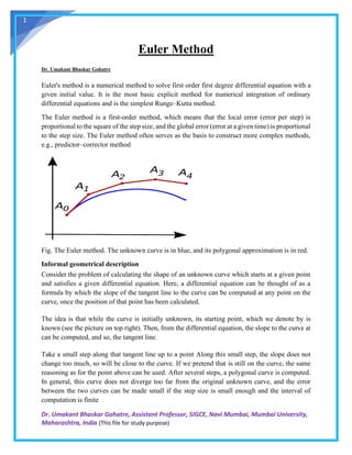
The document discusses Euler's method, a numerical technique for solving first-order differential equations with a given initial value, outlining its derivation, errors, and stability. It describes the process of approximating the curve of the solution through incremental steps based on calculated slopes, as well as the local and global truncation errors associated with the method. Additionally, it touches on the modifications and other related numerical methods, such as the backward Euler and midpoint methods.