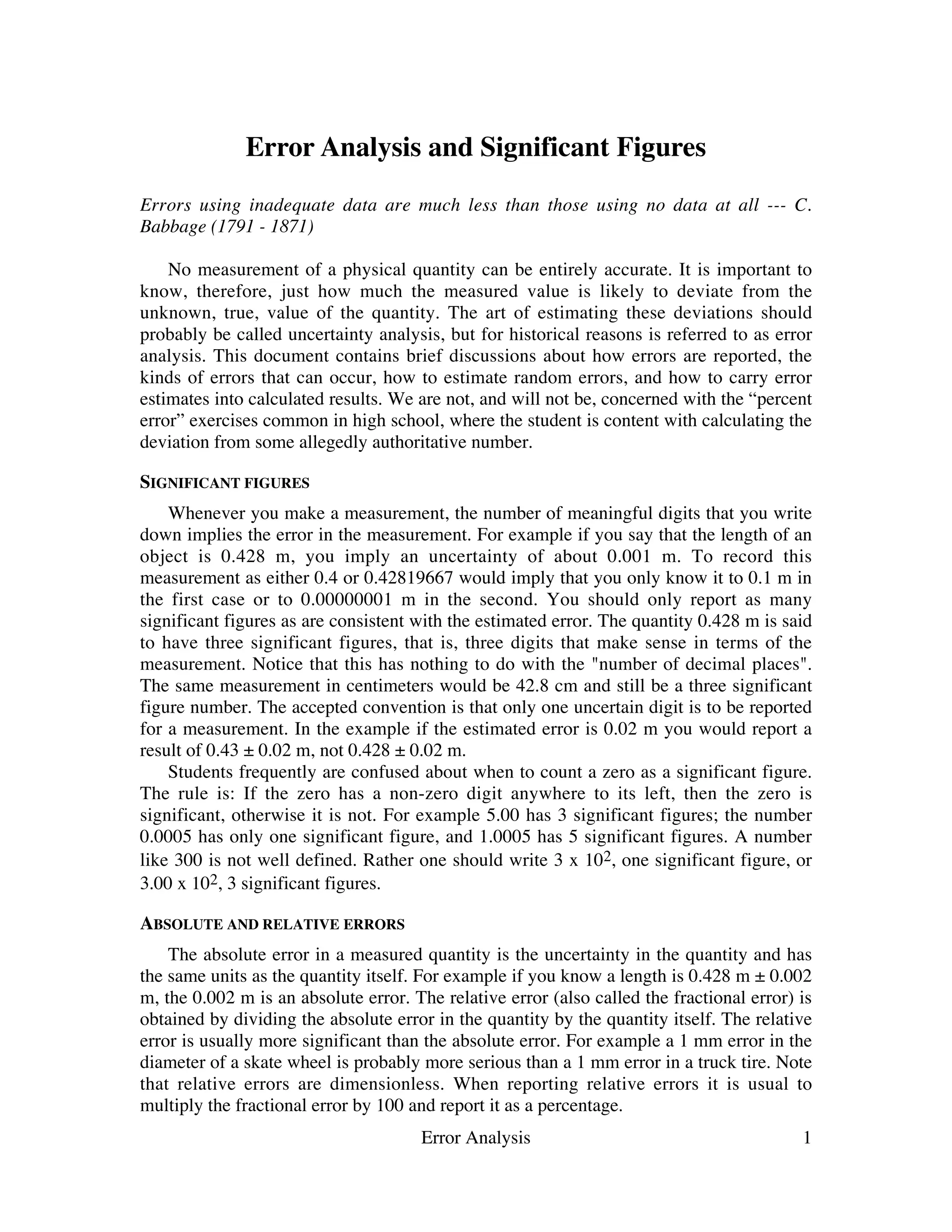
Error Analysis and Significant Figures 
Errors using inadequate data are much less than those using no data at all --- C. 
Babbage (1791 - 1871) 
No measurement of a physical quantity can be entirely accurate. It is important to 
know, therefore, just how much the measured value is likely to deviate from the 
unknown, true, value of the quantity. The art of estimating these deviations should 
probably be called uncertainty analysis, but for historical reasons is referred to as error 
analysis. This document contains brief discussions about how errors are reported, the 
kinds of errors that can occur, how to estimate random errors, and how to carry error 
estimates into calculated results. We are not, and will not be, concerned with the “percent 
error” exercises common in high school, where the student is content with calculating the 
deviation from some allegedly authoritative number. 
SIGNIFICANT FIGURES 
Whenever you make a measurement, the number of meaningful digits that you write 
down implies the error in the measurement. For example if you say that the length of an 
object is 0.428 m, you imply an uncertainty of about 0.001 m. To record this 
measurement as either 0.4 or 0.42819667 would imply that you only know it to 0.1 m in 
the first case or to 0.00000001 m in the second. You should only report as many 
significant figures as are consistent with the estimated error. The quantity 0.428 m is said 
to have three significant figures, that is, three digits that make sense in terms of the 
measurement. Notice that this has nothing to do with the "number of decimal places". 
The same measurement in centimeters would be 42.8 cm and still be a three significant 
figure number. The accepted convention is that only one uncertain digit is to be reported 
for a measurement. In the example if the estimated error is 0.02 m you would report a 
result of 0.43 ± 0.02 m, not 0.428 ± 0.02 m. 
Students frequently are confused about when to count a zero as a significant figure. 
The rule is: If the zero has a non-zero digit anywhere to its left, then the zero is 
significant, otherwise it is not. For example 5.00 has 3 significant figures; the number 
0.0005 has only one significant figure, and 1.0005 has 5 significant figures. A number 
like 300 is not well defined. Rather one should write 3 x 10², one significant figure, or 
3.00 x 10², 3 significant figures. 
ABSOLUTE AND RELATIVE ERRORS 
The absolute error in a measured quantity is the uncertainty in the quantity and has 
the same units as the quantity itself. For example if you know a length is 0.428 m ± 0.002 
m, the 0.002 m is an absolute error. The relative error (also called the fractional error) is 
obtained by dividing the absolute error in the quantity by the quantity itself. The relative 
error is usually more significant than the absolute error. For example a 1 mm error in the 
diameter of a skate wheel is probably more serious than a 1 mm error in a truck tire. Note 
that relative errors are dimensionless. When reporting relative errors it is usual to 
multiply the fractional error by 100 and report it as a percentage. 
Error Analysis 1
Error Analysis 2 
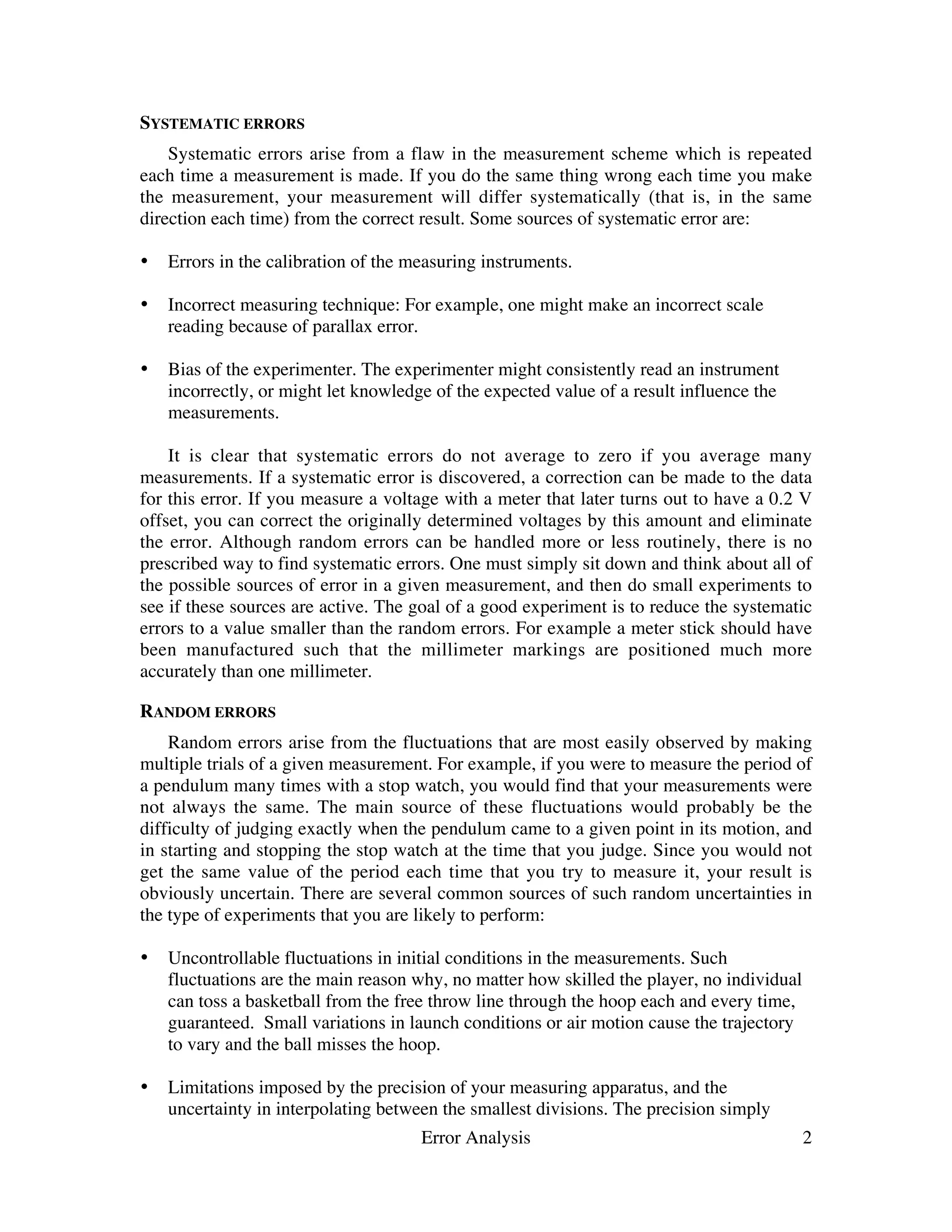
SYSTEMATIC ERRORS 
Systematic errors arise from a flaw in the measurement scheme which is repeated 
each time a measurement is made. If you do the same thing wrong each time you make 
the measurement, your measurement will differ systematically (that is, in the same 
direction each time) from the correct result. Some sources of systematic error are: 
• Errors in the calibration of the measuring instruments. 
• Incorrect measuring technique: For example, one might make an incorrect scale 
reading because of parallax error. 
• Bias of the experimenter. The experimenter might consistently read an instrument 
incorrectly, or might let knowledge of the expected value of a result influence the 
measurements. 
It is clear that systematic errors do not average to zero if you average many 
measurements. If a systematic error is discovered, a correction can be made to the data 
for this error. If you measure a voltage with a meter that later turns out to have a 0.2 V 
offset, you can correct the originally determined voltages by this amount and eliminate 
the error. Although random errors can be handled more or less routinely, there is no 
prescribed way to find systematic errors. One must simply sit down and think about all of 
the possible sources of error in a given measurement, and then do small experiments to 
see if these sources are active. The goal of a good experiment is to reduce the systematic 
errors to a value smaller than the random errors. For example a meter stick should have 
been manufactured such that the millimeter markings are positioned much more 
accurately than one millimeter. 
RANDOM ERRORS 
Random errors arise from the fluctuations that are most easily observed by making 
multiple trials of a given measurement. For example, if you were to measure the period of 
a pendulum many times with a stop watch, you would find that your measurements were 
not always the same. The main source of these fluctuations would probably be the 
difficulty of judging exactly when the pendulum came to a given point in its motion, and 
in starting and stopping the stop watch at the time that you judge. Since you would not 
get the same value of the period each time that you try to measure it, your result is 
obviously uncertain. There are several common sources of such random uncertainties in 
the type of experiments that you are likely to perform: 
• Uncontrollable fluctuations in initial conditions in the measurements. Such 
fluctuations are the main reason why, no matter how skilled the player, no individual 
can toss a basketball from the free throw line through the hoop each and every time, 
guaranteed. Small variations in launch conditions or air motion cause the trajectory 
to vary and the ball misses the hoop. 
• Limitations imposed by the precision of your measuring apparatus, and the 
uncertainty in interpolating between the smallest divisions. The precision simply
means the smallest amount that can be measured directly. A typical meter stick is 
subdivided into millimeters and its precision is thus one millimeter. 
• Lack of precise definition of the quantity being measured. The length of a table in the 
laboratory is not well defined after it has suffered years of use. You would find 
different lengths if you measured at different points on the table. Another possibility 
is that the quantity being measured also depends on an uncontrolled variable. (The 
temperature of the object for example). 
• Sometimes the quantity you measure is well defined but is subject to inherent random 
fluctuations. Such fluctuations may be of a quantum nature or arise from the fact that 
the values of the quantity being measured are determined by the statistical behavior of 
a large number of particles. Another example is AC noise causing the needle of a 
voltmeter to fluctuate. 
No matter what the source of the uncertainty, to be labeled "random" an uncertainty 
must have the property that the fluctuations from some "true" value are equally likely to 
be positive or negative. This fact gives us a key for understanding what to do about 
random errors. You could make a large number of measurements, and average the result. 
If the uncertainties are really equally likely to be positive or negative, you would expect 
that the average of a large number of measurements would be very near to the correct 
value of the quantity measured, since positive and negative fluctuations would tend to 
cancel each other. 
ESTIMATING RANDOM ERRORS 
There are several ways to make a reasonable estimate of the random error in a 
particular measurement. The best way is to make a series of measurements of a given 
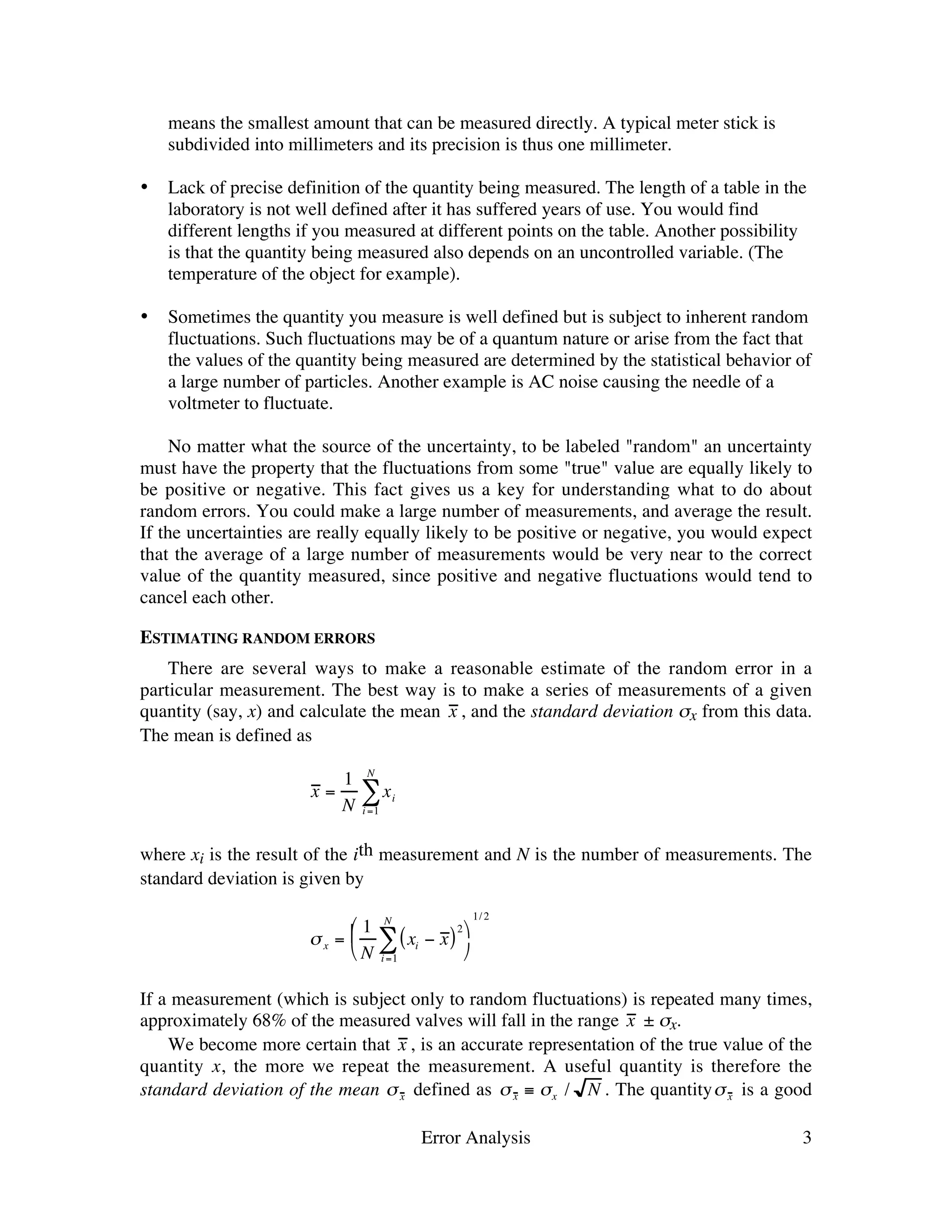
quantity (say, x) and calculate the mean x , and the standard deviation σx from this data. 
The mean is defined as 
NΣ where xi is the result of the ith measurement and N is the number of measurements. The 
Error Analysis 3 
x = 1 
N 
xi 
i =1 
standard deviation is given by 
σ x = 1 
N 
(xi − x )2 
NΣ 
i =1 
 
 
  
 
1/ 2 
If a measurement (which is subject only to random fluctuations) is repeated many times, 
approximately 68% of the measured valves will fall in the range x ± σx. 
We become more certain that x , is an accurate representation of the true value of the 
quantity x, the more we repeat the measurement. A useful quantity is therefore the 
standard deviation of the mean σ x defined as σ x ≡ σx / N . The quantityσ x is a good
estimate of our uncertainty in x . Notice that the measurement precision increases in 
proportion to N as we increase the number of measurements. Not only have you made 
a more accurate determination of the value, you also have a set of data that will allow you 
to estimate the uncertainty in your measurement. 
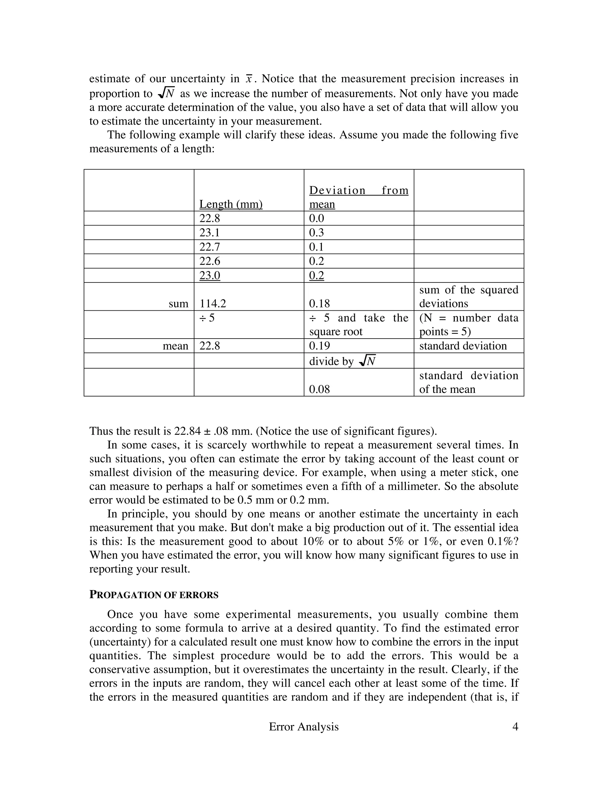
The following example will clarify these ideas. Assume you made the following five 
Error Analysis 4 
measurements of a length: 
Length (mm) 
Deviation from 
mean 
22.8 0.0 
23.1 0.3 
22.7 0.1 
22.6 0.2 
23.0 0.2 
sum 114.2 0.18 
sum of the squared 
deviations 
÷ 5 ÷ 5 and take the 
square root 
(N = number data 
points = 5) 
mean 22.8 0.19 standard deviation 
divide by N 
0.08 
standard deviation 
of the mean 
Thus the result is 22.84 ± .08 mm. (Notice the use of significant figures). 
In some cases, it is scarcely worthwhile to repeat a measurement several times. In 
such situations, you often can estimate the error by taking account of the least count or 
smallest division of the measuring device. For example, when using a meter stick, one 
can measure to perhaps a half or sometimes even a fifth of a millimeter. So the absolute 
error would be estimated to be 0.5 mm or 0.2 mm. 
In principle, you should by one means or another estimate the uncertainty in each 
measurement that you make. But don't make a big production out of it. The essential idea 
is this: Is the measurement good to about 10% or to about 5% or 1%, or even 0.1%? 
When you have estimated the error, you will know how many significant figures to use in 
reporting your result. 
PROPAGATION OF ERRORS 
Once you have some experimental measurements, you usually combine them 
according to some formula to arrive at a desired quantity. To find the estimated error 
(uncertainty) for a calculated result one must know how to combine the errors in the input 
quantities. The simplest procedure would be to add the errors. This would be a 
conservative assumption, but it overestimates the uncertainty in the result. Clearly, if the 
errors in the inputs are random, they will cancel each other at least some of the time. If 
the errors in the measured quantities are random and if they are independent (that is, if
one quantity is measured as being, say, larger than it really is, another quantity is still just 
as likely to be smaller or larger) then error theory shows that the uncertainty in a 
calculated result (the propagated error) can be obtained from a few simple rules, some of 
which are listed in Table I. For example if two or more numbers are to be added (Table 
I.2) then the absolute error in the result is the square root of the sum of the squares of the 
absolute errors of the inputs, i.e. 
if z = x + y 
then Δz = [(Δx)2 + (Δy)2 ]1/ 2 
In this and the following expressions, Δx and Δy are the absolute random errors in x and y 
and Δz is the propagated uncertainty in z. The formulas do not apply to systematic errors. 
The general formula, for your information, is the following; 
Σ  
Error Analysis 5 
(Δf (x1, x2 ,K ))2 
= 
δ f 
δ xi 
 
 
  
 
2 
Δxi ( )2 
It is discussed in detail in many texts on the theory of errors and the analysis of 
experimental data. For now, the collection of formulae on the next page will suffice.
TABLE I: PROPAGATED ERRORS IN z DUE TO ERRORS IN x and y. The errors in 
a, b and c are assumed to be negligible in the following formulae. 
Case/Function Propagated Error 
1) z = ax ± b Δz = aΔx 
2) z = x ± y Δz = (Δx)2 + (Δy)2 [ ]1/ 2 
 2 
 
 2 
 
 2 
 
Error Analysis 6 
3) z = cxy Δz 
z 
= 
Δx 
x 
 
 
 
 
2 
+ 
Δy 
y 
 
 
  
 
 
 
 
 
1/ 2 
4) z = c y 
x 
Δz 
z 
= 
Δx 
x 
 
 
 
 
2 
+ 
Δy 
y 
 
 
  
 
 
 
 
 
1/ 2 
5) z = cx a Δz 
z 
= a Δx 
x 
6) z = cx ayb Δz 
z 
= a Δx 
x 
 
 
 
 
2 
+ b Δy 
y 
 
 
  
 
 
 
 
 
1/ 2 
7) z = sin x Δz 
z 
= Δx cot x 
8) z = cos x Δz 
z 
= Δx tan x 
9) z = tan x Δz 
z 
= 
Δx 
sin x cos x

Error analysis

  • 1.
    Error Analysis andSignificant Figures Errors using inadequate data are much less than those using no data at all --- C. Babbage (1791 - 1871) No measurement of a physical quantity can be entirely accurate. It is important to know, therefore, just how much the measured value is likely to deviate from the unknown, true, value of the quantity. The art of estimating these deviations should probably be called uncertainty analysis, but for historical reasons is referred to as error analysis. This document contains brief discussions about how errors are reported, the kinds of errors that can occur, how to estimate random errors, and how to carry error estimates into calculated results. We are not, and will not be, concerned with the “percent error” exercises common in high school, where the student is content with calculating the deviation from some allegedly authoritative number. SIGNIFICANT FIGURES Whenever you make a measurement, the number of meaningful digits that you write down implies the error in the measurement. For example if you say that the length of an object is 0.428 m, you imply an uncertainty of about 0.001 m. To record this measurement as either 0.4 or 0.42819667 would imply that you only know it to 0.1 m in the first case or to 0.00000001 m in the second. You should only report as many significant figures as are consistent with the estimated error. The quantity 0.428 m is said to have three significant figures, that is, three digits that make sense in terms of the measurement. Notice that this has nothing to do with the "number of decimal places". The same measurement in centimeters would be 42.8 cm and still be a three significant figure number. The accepted convention is that only one uncertain digit is to be reported for a measurement. In the example if the estimated error is 0.02 m you would report a result of 0.43 ± 0.02 m, not 0.428 ± 0.02 m. Students frequently are confused about when to count a zero as a significant figure. The rule is: If the zero has a non-zero digit anywhere to its left, then the zero is significant, otherwise it is not. For example 5.00 has 3 significant figures; the number 0.0005 has only one significant figure, and 1.0005 has 5 significant figures. A number like 300 is not well defined. Rather one should write 3 x 10², one significant figure, or 3.00 x 10², 3 significant figures. ABSOLUTE AND RELATIVE ERRORS The absolute error in a measured quantity is the uncertainty in the quantity and has the same units as the quantity itself. For example if you know a length is 0.428 m ± 0.002 m, the 0.002 m is an absolute error. The relative error (also called the fractional error) is obtained by dividing the absolute error in the quantity by the quantity itself. The relative error is usually more significant than the absolute error. For example a 1 mm error in the diameter of a skate wheel is probably more serious than a 1 mm error in a truck tire. Note that relative errors are dimensionless. When reporting relative errors it is usual to multiply the fractional error by 100 and report it as a percentage. Error Analysis 1
  • 2.
    Error Analysis 2 SYSTEMATIC ERRORS Systematic errors arise from a flaw in the measurement scheme which is repeated each time a measurement is made. If you do the same thing wrong each time you make the measurement, your measurement will differ systematically (that is, in the same direction each time) from the correct result. Some sources of systematic error are: • Errors in the calibration of the measuring instruments. • Incorrect measuring technique: For example, one might make an incorrect scale reading because of parallax error. • Bias of the experimenter. The experimenter might consistently read an instrument incorrectly, or might let knowledge of the expected value of a result influence the measurements. It is clear that systematic errors do not average to zero if you average many measurements. If a systematic error is discovered, a correction can be made to the data for this error. If you measure a voltage with a meter that later turns out to have a 0.2 V offset, you can correct the originally determined voltages by this amount and eliminate the error. Although random errors can be handled more or less routinely, there is no prescribed way to find systematic errors. One must simply sit down and think about all of the possible sources of error in a given measurement, and then do small experiments to see if these sources are active. The goal of a good experiment is to reduce the systematic errors to a value smaller than the random errors. For example a meter stick should have been manufactured such that the millimeter markings are positioned much more accurately than one millimeter. RANDOM ERRORS Random errors arise from the fluctuations that are most easily observed by making multiple trials of a given measurement. For example, if you were to measure the period of a pendulum many times with a stop watch, you would find that your measurements were not always the same. The main source of these fluctuations would probably be the difficulty of judging exactly when the pendulum came to a given point in its motion, and in starting and stopping the stop watch at the time that you judge. Since you would not get the same value of the period each time that you try to measure it, your result is obviously uncertain. There are several common sources of such random uncertainties in the type of experiments that you are likely to perform: • Uncontrollable fluctuations in initial conditions in the measurements. Such fluctuations are the main reason why, no matter how skilled the player, no individual can toss a basketball from the free throw line through the hoop each and every time, guaranteed. Small variations in launch conditions or air motion cause the trajectory to vary and the ball misses the hoop. • Limitations imposed by the precision of your measuring apparatus, and the uncertainty in interpolating between the smallest divisions. The precision simply
  • 3.
    means the smallestamount that can be measured directly. A typical meter stick is subdivided into millimeters and its precision is thus one millimeter. • Lack of precise definition of the quantity being measured. The length of a table in the laboratory is not well defined after it has suffered years of use. You would find different lengths if you measured at different points on the table. Another possibility is that the quantity being measured also depends on an uncontrolled variable. (The temperature of the object for example). • Sometimes the quantity you measure is well defined but is subject to inherent random fluctuations. Such fluctuations may be of a quantum nature or arise from the fact that the values of the quantity being measured are determined by the statistical behavior of a large number of particles. Another example is AC noise causing the needle of a voltmeter to fluctuate. No matter what the source of the uncertainty, to be labeled "random" an uncertainty must have the property that the fluctuations from some "true" value are equally likely to be positive or negative. This fact gives us a key for understanding what to do about random errors. You could make a large number of measurements, and average the result. If the uncertainties are really equally likely to be positive or negative, you would expect that the average of a large number of measurements would be very near to the correct value of the quantity measured, since positive and negative fluctuations would tend to cancel each other. ESTIMATING RANDOM ERRORS There are several ways to make a reasonable estimate of the random error in a particular measurement. The best way is to make a series of measurements of a given quantity (say, x) and calculate the mean x , and the standard deviation σx from this data. The mean is defined as NΣ where xi is the result of the ith measurement and N is the number of measurements. The Error Analysis 3 x = 1 N xi i =1 standard deviation is given by σ x = 1 N (xi − x )2 NΣ i =1      1/ 2 If a measurement (which is subject only to random fluctuations) is repeated many times, approximately 68% of the measured valves will fall in the range x ± σx. We become more certain that x , is an accurate representation of the true value of the quantity x, the more we repeat the measurement. A useful quantity is therefore the standard deviation of the mean σ x defined as σ x ≡ σx / N . The quantityσ x is a good
  • 4.
    estimate of ouruncertainty in x . Notice that the measurement precision increases in proportion to N as we increase the number of measurements. Not only have you made a more accurate determination of the value, you also have a set of data that will allow you to estimate the uncertainty in your measurement. The following example will clarify these ideas. Assume you made the following five Error Analysis 4 measurements of a length: Length (mm) Deviation from mean 22.8 0.0 23.1 0.3 22.7 0.1 22.6 0.2 23.0 0.2 sum 114.2 0.18 sum of the squared deviations ÷ 5 ÷ 5 and take the square root (N = number data points = 5) mean 22.8 0.19 standard deviation divide by N 0.08 standard deviation of the mean Thus the result is 22.84 ± .08 mm. (Notice the use of significant figures). In some cases, it is scarcely worthwhile to repeat a measurement several times. In such situations, you often can estimate the error by taking account of the least count or smallest division of the measuring device. For example, when using a meter stick, one can measure to perhaps a half or sometimes even a fifth of a millimeter. So the absolute error would be estimated to be 0.5 mm or 0.2 mm. In principle, you should by one means or another estimate the uncertainty in each measurement that you make. But don't make a big production out of it. The essential idea is this: Is the measurement good to about 10% or to about 5% or 1%, or even 0.1%? When you have estimated the error, you will know how many significant figures to use in reporting your result. PROPAGATION OF ERRORS Once you have some experimental measurements, you usually combine them according to some formula to arrive at a desired quantity. To find the estimated error (uncertainty) for a calculated result one must know how to combine the errors in the input quantities. The simplest procedure would be to add the errors. This would be a conservative assumption, but it overestimates the uncertainty in the result. Clearly, if the errors in the inputs are random, they will cancel each other at least some of the time. If the errors in the measured quantities are random and if they are independent (that is, if
  • 5.
    one quantity ismeasured as being, say, larger than it really is, another quantity is still just as likely to be smaller or larger) then error theory shows that the uncertainty in a calculated result (the propagated error) can be obtained from a few simple rules, some of which are listed in Table I. For example if two or more numbers are to be added (Table I.2) then the absolute error in the result is the square root of the sum of the squares of the absolute errors of the inputs, i.e. if z = x + y then Δz = [(Δx)2 + (Δy)2 ]1/ 2 In this and the following expressions, Δx and Δy are the absolute random errors in x and y and Δz is the propagated uncertainty in z. The formulas do not apply to systematic errors. The general formula, for your information, is the following; Σ  Error Analysis 5 (Δf (x1, x2 ,K ))2 = δ f δ xi      2 Δxi ( )2 It is discussed in detail in many texts on the theory of errors and the analysis of experimental data. For now, the collection of formulae on the next page will suffice.
  • 6.
    TABLE I: PROPAGATEDERRORS IN z DUE TO ERRORS IN x and y. The errors in a, b and c are assumed to be negligible in the following formulae. Case/Function Propagated Error 1) z = ax ± b Δz = aΔx 2) z = x ± y Δz = (Δx)2 + (Δy)2 [ ]1/ 2  2   2   2  Error Analysis 6 3) z = cxy Δz z = Δx x     2 + Δy y          1/ 2 4) z = c y x Δz z = Δx x     2 + Δy y          1/ 2 5) z = cx a Δz z = a Δx x 6) z = cx ayb Δz z = a Δx x     2 + b Δy y          1/ 2 7) z = sin x Δz z = Δx cot x 8) z = cos x Δz z = Δx tan x 9) z = tan x Δz z = Δx sin x cos x