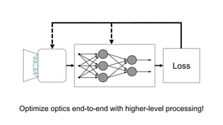
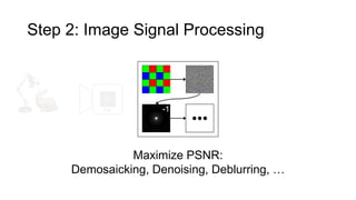
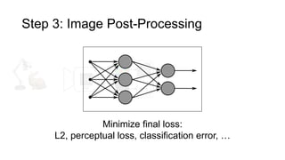
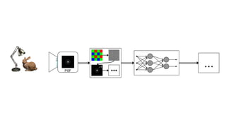
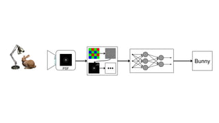
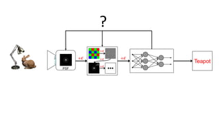
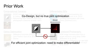
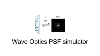
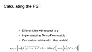
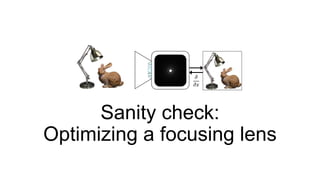
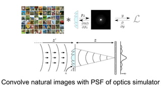
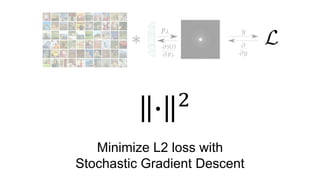
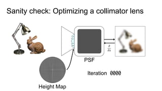
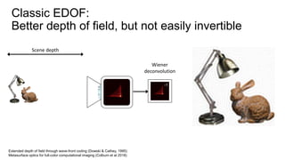
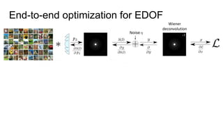
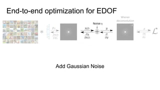
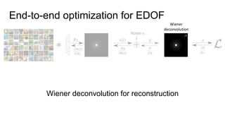
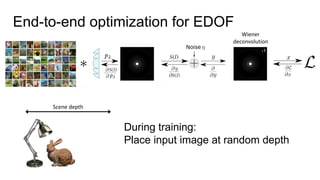
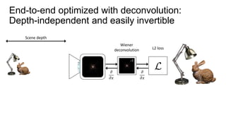
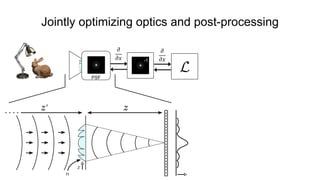
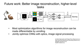
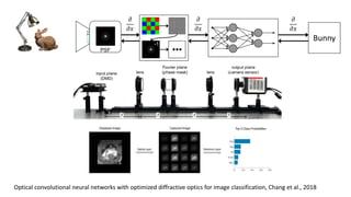
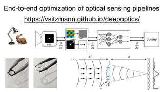
End-to-end Optimization of Optics and Image Processing for
Achromatic Extended Depth of Field and Super-Resolution
Imaging
Vincent Sitzmann*
Stanford University
Steven Diamond*
Stanford University
Yifan Peng*
University of
British Columbia
Xiong Dun
KAUST
Wolfgang Heidrich
KAUST
Stephen Boyd
Stanford University
Felix Heide
Stanford University
Gordon Wetzstein
Stanford University
Courtesy of Michael Bok Courtesy of CSIR Notes
Courtesy of MicrodacCourtesy of Jeffrey Beach
Loss
Optimize optics end-to-end with higher-level processing!
Regular bi-convex lens (focus close) Optimized camera
Results: Achromatic extended DOF
How do computer vision pipelines
work in real life?
What is this?
Step 1: Build camera
Optimize optics to minimize aberrations:
Blur/spot size, chromatic aberrations, distortions, …
Point Spread Function
(PSF)
Step 2: Image Signal Processing
Maximize PSNR:
Demosaicking, Denoising, Deblurring, …
PSF -1
Step 3: Image Post-Processing
Minimize final loss:
L2, perceptual loss, classification error, …
PSF
...PSF
-1
Bunny
PSF
-1
Teapot
?
PSF
-1
+ 𝜖 + 𝜖
+ 𝜖
+ 𝜖
+ 𝜖
𝜕
𝜕𝑥
𝜕
𝜕𝑥
Bunny
𝜕
𝜕𝑥
Vision: The Deep Computational Camera
Optimize end-to-end
PSF
-1
Bunny
𝜕
𝜕𝑥
Vision: The Deep Computational Camera
• Performance & robustness gains
• Domain-specific hardware may reduce footprint, cost, power…
• New design space: The “BunnyCam”
𝜕
𝜕𝑥
PSF
𝜕
𝜕𝑥
-1
Bunny
𝜕
𝜕𝑥
This project: Enable optimization of optics!
𝜕
𝜕𝑥
PSF
𝜕
𝜕𝑥
-1
Prior Work
Computational Cameras
Optics Optimization
Differentiable ISPs
Deep Computational Photography
• Deep Joint Demosaicking and
Denoising (Gharbi et al. 2016)
• Unrolled Optimiziation with Deep
Priors (Diamond et al.)
• …
• EDOF through wave-front coding (Dowski
& Cathey, 1995)
• Recovering HDR radiance maps from
photographs (Debevec & Malik 1997)
• …
• Diffractive Achromat (Peng et al. 2016)
• Lens Factory (Sun et al. 2015)
• Zemax
• …
• HDR image reconstruction from a
single exposure using deep CNNs
(Eiltertsen et al. 2016)
• Learning to synthesize a 4d rgbd light
field from a single image (Srinivasan
et al. 2017)
• …
-1
Co-Design, but no true joint optimization
Wiener
deconvolution
For efficient joint optimization: need to make differentiable!
A differentiable optics model
𝜕
𝜕𝑥
PSF
Image formation model
* =+
How does the optical element map to the PSF?
?
* =+
𝜕
𝜕𝑥
Wave Optics PSF simulator
PSF𝜕
𝜕𝑥
Spherical wave from point source
Phaseshift by optical element
𝑈 𝑥 = exp 𝑗𝑘 𝑥2 + 𝑧′2 + 𝑛 − 1 Φ x
Phaseshift by optical element
𝑈 𝑥 = exp 𝑗𝑘 𝑥2 + 𝑧′2 + 𝑛 − 1 Φ x
Phaseshift by optical element
Φ
𝑈 𝑥 = exp 𝑗𝑘 𝑥2 + 𝑧′2 + 𝑛 − 1 Φ x
Height Map parameterization
(diffractive)
Zernike basis parameterization
(refractive)
Φ 𝑥 = [ 𝑎11, 𝑎12, … , … ] Φ[𝑥] = 𝑍𝑖
𝑗
𝑥 ∙ 𝑎𝑖𝑗
Phaseshift by optical element
Φ
𝑈 𝑥 = exp 𝑗𝑘 𝑥2 + 𝑧′2 + 𝑛 − 1 Φ x
Fresnel propagation to sensor
𝑈′
𝑥 = 𝑈 𝑥 ∗ exp(
𝑗𝑘
2𝑧
𝑥2
)
Intensity measurement at sensor
𝑈′
𝑥 2
PSF
𝜌 𝑧′,𝜆 = exp 𝑗𝑘 𝑥2 + 𝑦2 + 𝑧′2 + 𝑛 − 1 𝜙 𝑥, 𝑦 ∗ exp 𝑗
𝑘
2𝑧
𝑥2
+ 𝑦2
2
Calculating the PSF
PSF
Calculating the PSF
𝜌 𝑧′,𝜆 = exp 𝑗𝑘 𝑥2 + 𝑦2 + 𝑧′2 + 𝑛 − 1 𝜙 𝑥, 𝑦 ∗ exp 𝑗
𝑘
2𝑧
𝑥2
+ 𝑦2
2
• Differentiable with respect to 𝜙
• Implemented as TensorFlow module
• Can easily combine with other models!
Sanity check:
Optimizing a focusing lens
𝜕
𝜕𝑥
Convolve natural images with PSF of optics simulator
Minimize L2 loss with
Stochastic Gradient Descent
∙ 2
Sanity check: Optimizing a collimator lens
𝜕
𝜕𝑥
Iteration
Height Map
PSF
Fabrication
Refractive: Single-point Diamond TurningDiffractive: Photolithography
Application: Achromatic EDOF
Problem with single lens:
Limited Depth of Field, chromatic aberrations
Scene depth
Focal plane
Classic EDOF:
Better depth of field, but not easily invertible
Scene depth
Wiener
deconvolution
-1
Extended depth of field through wave-front coding (Dowski & Cathey, 1995)
Metasurface optics for full-color computational imaging (Colburn et al 2018)
End-to-end optimization for EDOF
-1
Wiener
deconvolution
-1
Wiener
deconvolution
Add Gaussian Noise
End-to-end optimization for EDOF
-1
Wiener
deconvolution
Wiener deconvolution for reconstruction
End-to-end optimization for EDOF
Scene depth
During training:
Place input image at random depth
-1
Wiener
deconvolution
End-to-end optimization for EDOF
End-to-end optimized with deconvolution:
Depth-independent and easily invertible
Scene depth
𝜕
𝜕𝑥
Wiener
deconvolution
𝜕
𝜕𝑥
L2 loss
Fresnel Lens
Multifocal
Lens
Cubic Phase
Plate
Diffractive
Achromat
Refr. / Diffr.
Hybrid Lens
Ours
17.95 dB 18.32 18.33 20.20 18.92 24.30
-1
Refractive Achromatic EDOF element
• Polymethyl methacrylate (PMMA)
• 5 mm aperture size
• Sensor distance 35.5𝑚𝑚
• F-number 7.1
• One active optical surface
• Feature size 3.69𝜇𝑚
Optical surface
Caustics
Regular bi-convex lens Optimized lens
Elephant (0.5m) Book (2.0m)
Sensor image
Test scene
Processed image
Regular bi-convex lens Optimized lens
Elephant (0.5m) Book (2.0m)
Test scene
Regular bi-convex lens (focus close) Optimized camera
Real-world capture
Diffractive Achromatic EDOF element
• Fused silica processed via 16-level
photolithography
• 5 mm aperture size
• Sensor distance 35.5𝑚𝑚
• F-number 7.1
• One active optical surface
• Feature size 2𝜇𝑚
Regular Fresnel Lens Optimized Camera w. diffractive element
Diffractive EDOF: Test scene
Experimental application: Super-Resolution
Please refer to paper for more detail!
Summary
-1
𝜕
𝜕𝑥
Jointly optimizing optics and post-processing
PSF
𝜕
𝜕𝑥
𝜕
𝜕𝑥
Bunny
𝜕
𝜕𝑥
𝜕
𝜕𝑥
PSF
-1
• Most optimization algorithms for image reconstruction can be
made differentiable by unrolling
• Jointly optimize CNNs with optics, image signal processing
Future work: Better image reconstruction, higher-level
tasks
Unrolled Optimization with Deep Priors (Diamond et al.)
Deep Joint Demosaicking and Denoising (Gharbi et al.)
DeepISP (Schwartz et al.)
FlexISP (Heide et al.)
…
Bunny
PSF
Optical convolutional neural networks with optimized diffractive optics for image classification, Chang et al., 2018
-1
𝜕
𝜕𝑥
𝜕
𝜕𝑥
𝜕
𝜕𝑥
Felix Heide
Evan Peng Wolfgang Heidrich
Stephen Boyd Gordon Wetzstein
Xiong Dun
End-to-end optimization of optical sensing pipelines
https://vsitzmann.github.io/deepoptics/
𝜕
𝜕𝑥
Bunny
𝜕
𝜕𝑥
𝜕
𝜕𝑥
PSF
-1

End-to-end Optimization of Cameras and Image Processing - SIGGRAPH 2018

Editor's Notes

  • #2 Welcome everyone…
  • #3 In the animal kingdom, eyes have co-evolved with the brain to form a vibrant variety of domain-specific visual systems.
  • #4 In contrast, while our computer vision pipelines solve widely different problems, they all follow the same fundamental approach of creating a sharp image on a sensor before processing it.
  • #5 Instead, we propose to jointly optimize the camera optics with the brain of our computer vision pipelines – the algorithms.
  • #6 We can then fabricate the optimized lenses with state-of-the-art manufacturing techniques such as single-point diamond turning.
  • #7 We’ll show you how to use these elements to address real-world challenges such as extended depth of field.
  • #8 To get started, let’s briefly think about how computer vision pipelines work in the real world.
  • #9 Let’s say we wanted to classify this scene – a bunny.
  • #10 The first step is to build a camera. Let‘s focus on the camera optics, characterized by its Point Spread Function, which is the impulse response of the optics. We will optimize the PSF for blur and spot size, chromatic aberrations, distortions etc., to get a sharp image with little aberrations on the sensor.
  • #11 In the next step, we design image signal processing, such as Demosaicing, Denoising, Deblurring etc., to maximize the PSNR and make a nice looking image.
  • #12 Lastly, we stick that image into some higher-level algorithm, such as a convolutional neural network, and optimize that for the domain-specific task we‘re trying to solve.
  • #14 And then, hopefully, it works!
  • #15 Except, of course, when it doesn‘t. Along each step of the pipeline, error can accumulate, and information that may be relevant to downstream tasks can be thrown away. There‘s no way for downstream tasks to feed back what information it needs!
  • #16 With this work, we follow the paradimg of optimizing this whole pipeline end-to-end.
  • #18 We focus on the optics with simple processing. We‘ll show you steps towards this vision.
  • #20 So, let’s talk about how we arrive at a differentiable camera model.
  • #21 Let’s zoom into our camera and look at what’s going on inside. The true (or latent) image is first convolved with the PSF, determined by the optics. The sensor then adds noise, so that we measure a blurred, noisy version of the true image.
  • #22 We now need to find a way to compute the PSF of our optical system in a differentiable manner, so that we can compute gradients of the PSF with respect to some parameterization of the optics.
  • #23 To this end, we contribute the differentiable wave optics PSF simulator.
  • #24 Let’s assume there’s a light point source at a fixed distance z prime to the left. It emits a spherical wave. At distance z’, the phase of the spherical wave can be described by the squared phase term below.
  • #25 The wave now hits the optical element. The optical element is represented here as a thickness function phi. Depending on its refractive index, the lens locally shifts the phase of the incoming wavefront, so that after the optical element, the wavefront is described by the term below.
  • #26 The wave now hits the optical element. The optical element is represented here as a thickness function phi. Depending on its refractive index, the lens locally shifts the phase of the incoming wavefront, so that after the optical element, the wavefront is described by the term below.
  • #27 The wave now hits the optical element. The optical element is represented here as a thickness function phi. Depending on its refractive index, the lens locally shifts the phase of the incoming wavefront, so that after the optical element, the wavefront is described by the term below.
  • #29 The optical element can be parameterized in a variety of ways. We parameterized diffractive elements directly via a “height map”, i.e., simply a discretized grid that contains the thickness of the element at each spatial position, and a Zernike basis representation.
  • #30 In the next step, the wave propagates from the aperture to the sensor. Since we are interested in an arbitrary optical element, there is no simple analytical form of this process. Instead, we have to compute the Fresnel propagation integral, which is equivalent to computing a convolution with the Fresnel propagation kernel. This is the operator to propagate light through free space.
  • #31 Finally, the wavefront hits the sensor, which measures the intensity, or squared absolute, of the wavefront. Since the source of our wave was a point source at a distance z prime and of a wavelength lambda, this intensity image is equivalent to the PSF of the system for that depth and wavelength.
  • #34 Now lets see how the optimization pipeline works for the simple task of learning a focusing lens.
  • #35 We use a database of natural images, which we convolve with the PSF generated by the optics simulator to get the sensor output.
  • #36 We apply an L2 loss to the difference between the sensor output and the input image. We optimize the pipeline for the L2 loss using stochastic gradient descent.
  • #37 Here you can see the SGD algorithm running. The PSF converges to a point, the sensor output converges to a sharp image, and the optical element height map converges to a pattern like a Fresnel element.
  • #38 We manufactured the lenses we optimized in simulation using two procedures: photolithography for diffractive lenses, on the left, and diamond turning for refractive lenses, on the right.
  • #39 Here you can see a diffractive lens we optimized and manufactured, on the right, and a refractive lens, on the left.
  • #40 I’ll now go in detail through our application of optimizing a single lens imaging system for achromatic extended depth of field.
  • #41 Single lens cameras have limited depth of field, meaning the range within which an object is sharp is limited, and suffer from chromatic aberrations, or different focal points for different colors.
  • #42 Classic EDOF hand-engineers a depth-independent PSF. However, the PSF engineering has no knowledge of what PSF is easily invertible, as well as the tradeoff of which changes across depth are acceptable versus which ones may break the deconvolution algorithm. This leads to deconvolution artifacts in the reconstructed image.
  • #43 To tackle this problem with our pipeline, we extend the basic focusing lens case with two further steps.
  • #44 We model sensor noise by adding gaussian noise to the image after PSF blur is applied.
  • #45 We then use wiener deconvolution as an image reconstruction algorithm. Wiener deconvolution has an analytical solution and is thus easily differentiated through.
  • #46 We place the sampled images at random depths while running the SGD algorithm. That way we optimize over all depths in expectation.
  • #47 Our optimized imaging system substantially outperforms alternative approaches in simulation, measured by the PSNR of the reconstructed image.
  • #48 We manufactured the optimized lens as a refractive element. You can see from the caustics that the PSF is not simple or obvious. The lens was made out of PMMA, and has an F-number of 7.1.
  • #49 Here we show a test scene captured with a regular bi-convex lens, on the left, and our optimized refractive lens, on the right. The image on the right is that cast on the sensor, before reconstruction. Our optimization does not care about this image, except to the extent that it affects the final reconstructed output. That’s why the image is blurry, but with an approximately depth invariant blur.
  • #50 Now you can see the reconstructed image on the right. The image is sharp and in focus over the entire depth range, and for all colors.
  • #51 Here’s a real world capture with Vincent charging at the camera. On the left, we focused a bi-convex lens close to the camera. On the right, we used our optimized lens with reconstruction. Both lenses have the same F-number.
  • #52 We also optimized and manufactured a diffractive element for achromatic EDOF. Again, you can see the PSF is non-trivial. The lens was made using 16 level photolithography, and has an F-number of 7.1.
  • #53 Here is a test scene captured with a Fresnel lens, on the left, and the optimized diffractive element, on the right. The image on the right includes reconstruction. The output of our optimized pipeline is sharper than the Fresnel lens baseline, though both lenses suffer from haze and other effects common with diffractive elements.
  • #54 We also looked at the more experimental application of super-resolution. We tested whether the optimization pipeline could learn unconventional PSFs. In this case, the pipeline learned to multiplex the image onto three different locations on the camera. You can read about the details in the paper.
  • #55 We also looked at the more experimental application of super-resolution. We tested whether the optimization pipeline could learn unconventional PSFs. In this case, the pipeline learned to multiplex the image onto three different locations on the camera. You can read about the details in the paper.
  • #57 With this project we enable joint optimization of camera optics with higher-level processing by building a differentiable optics simulator that can simply be placed in an end-to-end optimization pipeline.
  • #58 While in this project, we focused on the optics and thus only considered simple post-processing algorithms and tasks, we are working on optimizing the whole camera pipeline end-to-end with more advanced post-processing algorithms, such as neural networks and differentiable unrolled optimization algorithms.
  • #59 More recently, our colleague Julie has used differentiable optics to optimize for the first layer of a convolutional neural network, thereby saving computation and power. Check it out!
  • #60 We thank our collaborators at KAUST and Stanford.
  • #61 We’ve made our code publically available on Github. We welcome questions!