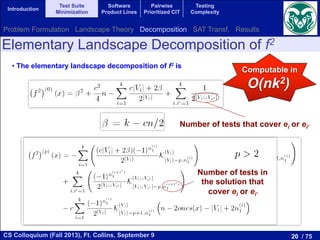
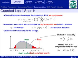
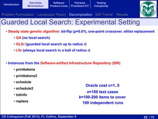
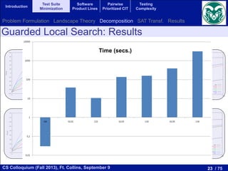
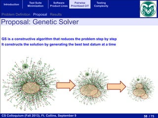
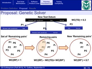
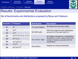
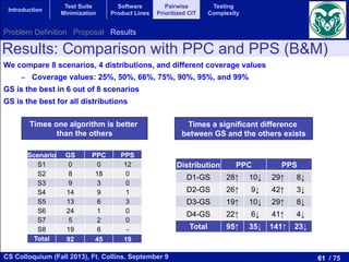
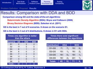
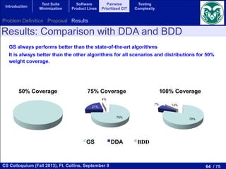
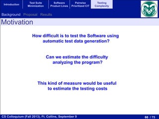
The document discusses recent advancements in test suite minimization within software testing, emphasizing optimization problems and techniques such as evolutionary algorithms and search-based software engineering (SBSE). It outlines the significance of software testing, various testing techniques, and challenges associated with regression testing. Additionally, it highlights the relationship between satisfiability problems and optimization algorithms, advocating the use of advanced SAT solvers for addressing these challenges.


![14 / 75CS Colloquium (Fall 2013), Ft. Collins, September 9
Introduction
Test Suite
Minimization
Software
Product Lines
Pairwise
Prioritized CIT
Testing
Complexity
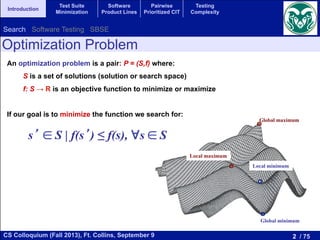
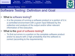
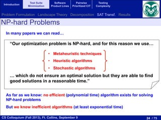
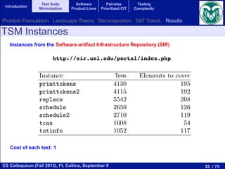
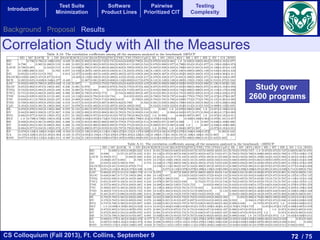
Test Suite Minimization
Given:
# A set of test cases T = {t1, t2, ..., tn}
# A set of program elements to be covered (e.g., branches) E= {e1, e2, ..., ek}
# A coverage matrix
Find a subset of tests X ⊆ T maximizing coverage and minimizing the testing cost
The single-objective version of this problem consists in finding a subset of
sts X ✓ T with minimum cost covering all the program elements. In formal
rms:
minimize cost(X) =
nX
i=1
ti2X
ci (2)
ubject to:
ej 2 E, 9ti 2 X such that element ej is covered by test ti, that is, mij = 1.
The multi-objective version of the TSMP does not impose the constraint of
ll coverage, but it defines the coverage as the second objective to optimize,
ading to a bi-objective problem. In short, the bi-objective TSMP consists in
nding a subset of tests X ✓ T having minimum cost and maximum coverage.
ormally:
minimize cost(X) =
nX
i=1
ti2X
ci (3)
maximize cov(X) = |{ej 2 E|9ti 2 X with mij = 1}| (4)
e1 e2 e3 ... ek
t1 1 0 1 … 1
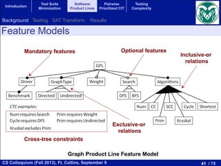
t2 0 0 1 … 0
… … … … … …
tn 1 1 0 … 0
M=
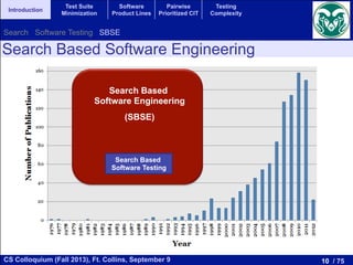
3 Test Suite Minimization Problem
When a piece of software is modified, the new software is tested using
previous test cases in order to check if new errors were introduced. This
is known as regression testing. One problem related to regression testing
Test Suite Minimization Problem (TSMP). This problem is equivalent t
Minimal Hitting Set Problem which is NP-hard [17]. Let T = {t1, t2, · · ·
be a set of tests for a program where the cost of running test ti is ci an
E = {e1, e2, · · · , em} be a set of elements of the program that we want to
with the tests. After running all the tests T we find that each test can
several program elements. This information is stored in a matrix M = [m
dimension n ⇥ m that is defined as:
mij =
(
1 if element ej is covered by test ti
0 otherwise
The single-objective version of this problem consists in finding a subs
tests X ✓ T with minimum cost covering all the program elements. In fo
terms:
minimize cost(X) =
nX
i=1
ti2X
ci
subject to:
8ej 2 E, 9ti 2 X such that element ej is covered by test ti, that is, mi
Yoo & Harman
Problem Formulation Landscape Theory Decomposition SAT Transf. Results](https://image.slidesharecdn.com/cs-csu-chicano-140709093451-phpapp02/85/Recent-Research-in-Search-Based-Software-Testing-14-320.jpg)
![30 / 75CS Colloquium (Fall 2013), Ft. Collins, September 9
Introduction
Test Suite
Minimization
Software
Product Lines
Pairwise
Prioritized CIT
Testing
Complexity
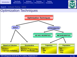
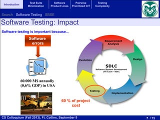
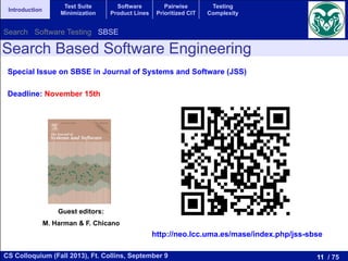
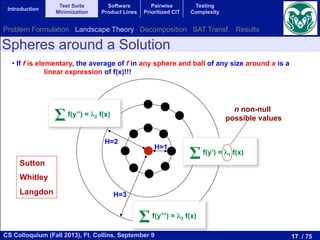
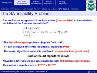
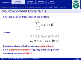
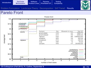
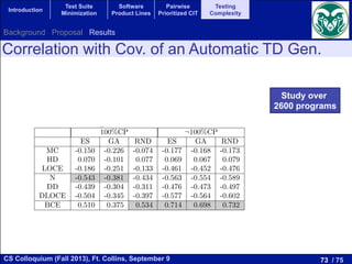
PB Constraints for the TSM Problem
e1 e2 e3 ... em
t1 1 0 1 … 1
t2 0 0 1 … 0
… … … … … …
tn 1 1 0 … 0
M=
previous test cases in order to check if new errors were introduced. This
is known as regression testing. One problem related to regression testing
Test Suite Minimization Problem (TSMP). This problem is equivalent t
Minimal Hitting Set Problem which is NP-hard [17]. Let T = {t1, t2, · · ·
be a set of tests for a program where the cost of running test ti is ci an
E = {e1, e2, · · · , em} be a set of elements of the program that we want to
with the tests. After running all the tests T we find that each test can
several program elements. This information is stored in a matrix M = [m
dimension n ⇥ m that is defined as:
mij =
(
1 if element ej is covered by test ti
0 otherwise
The single-objective version of this problem consists in finding a subs
tests X ✓ T with minimum cost covering all the program elements. In fo
terms:
minimize cost(X) =
nX
i=1
ti2X
ci
subject to:
8ej 2 E, 9ti 2 X such that element ej is covered by test ti, that is, mi
The multi-objective version of the TSMP does not impose the constra
full coverage, but it defines the coverage as the second objective to opti
leading to a bi-objective problem. In short, the bi-objective TSMP consi
finding a subset of tests X ✓ T having minimum cost and maximum cove
Formally:
n
ase is not included. We also introduce m binary variables e
ch program element to cover. If ej = 1 then the correspondin
by one of the selected test cases and if ej = 0 the elem
y a selected test case.
lues of the ej variables are not independent of the ti variable
j must be 1 if and only if there exists a ti variable for whic
1. The dependence between both sets of variables can be wr
ing 2m PB constraints:
ej
nX
i=1
mijti n · ej 1 j m.
n see that if the sum in the middle is zero (no test is co
j) then the variable ej = 0. However, if the sum is greater
ow we need to introduce a constraint related to each objectiv
o transform the optimization problem in a decision probl
in Section 2.2. These constraints are:
variables are not independent of the ti variables. A given
and only if there exists a ti variable for which mij = 1
ence between both sets of variables can be written with
nstraints:
nX
i=1
mijti n · ej 1 j m. (5)
the sum in the middle is zero (no test is covering the
ariable ej = 0. However, if the sum is greater than zero
introduce a constraint related to each objective function
the optimization problem in a decision problem, as we
. These constraints are:
nX
i=1
citi B, (6)
mX
the following 2m PB constraints:
ej
nX
i=1
mijti n · ej 1 j
We can see that if the sum in the middle is zero (no
element ej) then the variable ej = 0. However, if the sum
ej = 1. Now we need to introduce a constraint related to ea
in order to transform the optimization problem in a dec
described in Section 2.2. These constraints are:
nX
i=1
citi B,
mX
j=1
ej P,
Cost Coverage
Problem Formulation Landscape Theory Decomposition SAT Transf. Results](https://image.slidesharecdn.com/cs-csu-chicano-140709093451-phpapp02/85/Recent-Research-in-Search-Based-Software-Testing-30-320.jpg)

![44 / 75CS Colloquium (Fall 2013), Ft. Collins, September 9
Introduction
Test Suite
Minimization
Software
Product Lines
Pairwise
Prioritized CIT
Testing
Complexity
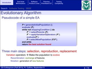
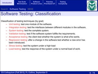
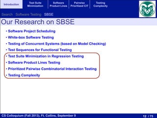
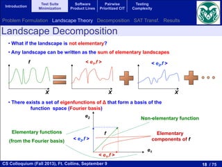
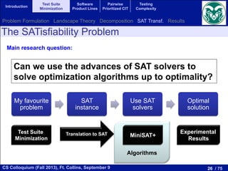
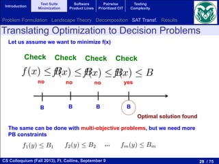
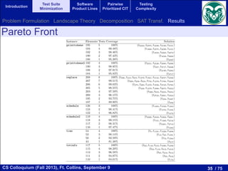
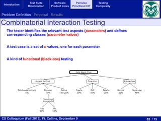
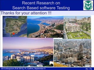
Testing of SPLs: Multi-Objective Formulation
If we don’t have the resources to run all the tests, which one to choose?
Multi-objective formulation:
minimize the number of products
maximize the coverage (t-wise interactions)
The solution is not anymore a table of products, but a Pareto set
by the number of variables dj,k,l that
as:
1X
=1
fX
k=j+1
3X
l=0
dj,k,l (7)
rogram is composed of the goal (7)
(f 1) constraints given by (2) to (6)
he FM expressed with the inequalities
e number of variables of the program
). The solution to this zero-one linear
with the maximum coverage that can
ucts.
ALGORITHM
e for obtaining the optimal Pareto set
This algorithm takes as input the FM
l Pareto set. It starts by adding to the
always in the set: the empty solution
one arbitrary solution (with coverage
ons of the set of features). After that
h successive zero-one linear programs
creasing number of products starting
l model is solved using a extended
. This solver provides a test suite with
This solution is stored in the optimal
m stops when adding a new product to
crease the coverage. The result is the
EXPERIMENTS
s how the evaluation was carried out
sis. The experimental corpus of our
y a benchmark of 118 feature models,
ts ranges from 16 to 640 products, that
om the SPL Conqueror [16] and the
s. The objectives to optimize are the
//minisat.se/MiniSat+.html
want the algorithm to be as fast as possible. For comparison
these experiments were run in a cluster of 16 machines with
Intel Core2 Quad processors Q9400 at 2.66 GHz and 4 GB
running Ubuntu 12.04.1 LTS managed by the HT Condor 7.8.4
manager. Each experiment was executed in one core.
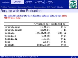
We computed the Pareto optimal front for each model.
Figure 2 shows this front for our running example GPL,
where the total coverage is obtained with 12 products, and
for every test suite size the obtained coverage is also optimal.
As our approach is able to compute the Pareto optimal front
for every feature model in our corpus, it makes no sense to
analyze the quality of the solutions. Instead, we consider more
interesting to study the scalability of our approach. For that,
we analyzed the execution time of the algorithm as a function
of the number of products represented by the feature model as
shown in Figure 3. In this figure we can observe a tendency:
the higher the number of products, the higher the execution
time. Although it cannot be clearly appreciated in the figure,
the execution time does not grow linearly with the number of
products, the growth is faster than linear.
Fig. 2. Pareto optimal front for our running example (GPL).
GPL
2-wise interactions
Background Testing SAT Transform. Results](https://image.slidesharecdn.com/cs-csu-chicano-140709093451-phpapp02/85/Recent-Research-in-Search-Based-Software-Testing-44-320.jpg)
![49 / 75CS Colloquium (Fall 2013), Ft. Collins, September 9
Introduction
Test Suite
Minimization
Software
Product Lines
Pairwise
Prioritized CIT
Testing
Complexity
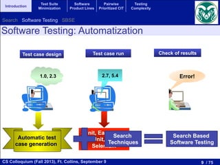
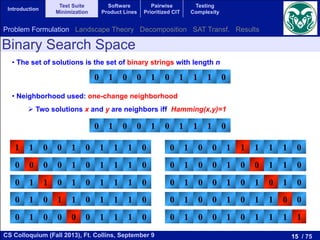
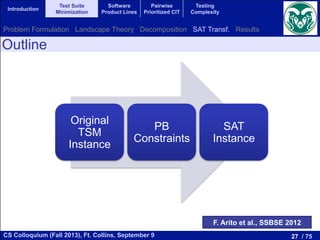
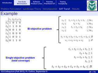
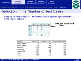
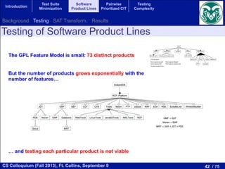
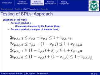
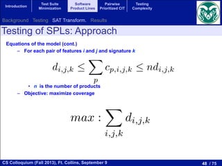
Testing of SPLs: Approach
f:
,k,0 (2)
(3)
(4)
(5)
product.
when all
d dj,k,l,
k with
herwise.
he dj,k,l
lities for
Algorithm 1 Algorithm for obtaining the optimal Pareto set.
optimal set {;};
cov[0] 0;
cov[1] Cf
2 ;
sol arbitraryValidSolution(fm);
i 1;
while cov[i] 6= cov[i 1] do
optimal set optimal set [ {sol};
i i + 1;
m prepareMathModel(fm,i);
sol solveMathModel(m);
cov[i] |sol|;
end while
number of products required to test the SPL and the achieved
Background Testing SAT Transform. Results](https://image.slidesharecdn.com/cs-csu-chicano-140709093451-phpapp02/85/Recent-Research-in-Search-Based-Software-Testing-49-320.jpg)
![50 / 75CS Colloquium (Fall 2013), Ft. Collins, September 9
Introduction
Test Suite
Minimization
Software
Product Lines
Pairwise
Prioritized CIT
Testing
Complexity
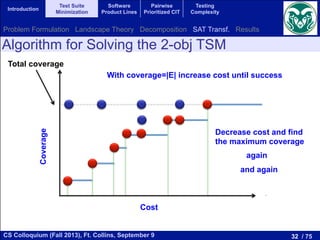
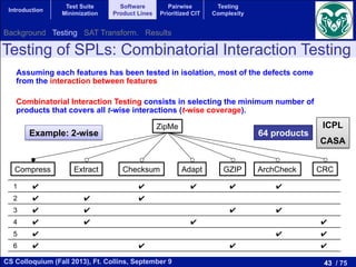
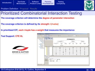
Testing of SPLs: Results
of the redundant constraints can incr
adding more constraints could help th
a solution. We plan to study the right b
and augmenting constraints. Second,
feature models to further study the sca
ACKNOWLEDGEME
Funded by Austrian Science Fund
N15 and Lise Meitner Fellowship M
Ministry of Economy and Competitive
contract TIN2011-28194 and fellowsh
REFERENCES
[1] P. Zave, “Faq sheet on
http://www.research.att.com/ pamela/faq.h
[2] K. Pohl, G. Bockle, and F. J. van der L
Engineering: Foundations, Principles and
Experiments on 118 feature models taken from
SPLOT repository (http://www.splot-research.org)
SPL Conqueror (http://wwwiti.cs.uni-magdeburg.de/~nsiegmun/SPLConqueror/)
16 to 640 products
Intel Core2 Quad Q9400
2.66 GHz, 4 GB
Background Testing SAT Transform. Results](https://image.slidesharecdn.com/cs-csu-chicano-140709093451-phpapp02/85/Recent-Research-in-Search-Based-Software-Testing-50-320.jpg)


![68 / 75CS Colloquium (Fall 2013), Ft. Collins, September 9
Introduction
Test Suite
Minimization
Software
Product Lines
Pairwise
Prioritized CIT
Testing
Complexity
Other Measures
measure in use. An examination of the main metrics reveals that most of them confuse the complexity
of a program with its size. The underlying idea of these measures are that a program will be much more
di cult to work with than a second one if, for example, it is twice the size, has twice as many control paths
leading through it, or contains twice as many logical decisions. Unfortunately, these various ways in which
a program may increase in complexity tend to move in unison, making it di cult to identify the multiple
dimensions of complexity.
In this section we present the measures used in this study. In a first group we select the main measures
that we found in the literature:
• Lines of Code (LOC)
• Source Lines of Code (SLOC)
• Lines of Code Equivalent (LOCE)
• Total Number of Disjunctions (TNDj)
• Total Number of Conjunctions (TNCj)
• Total Number of Equalities (TNE)
• Total Number of Inequalities (TNI )
• Total Number of Decisions (TND)
• Number of Atomic Conditions per Decision (CpD)
• Nesting Degree (N )
• Halstead’s Complexity (HD)
• McCabe’s Cyclomatic Complexity (MC)
Let’s have a look at the measures that are directly based on source lines of code (in C-based languages).
The LOC measure is a count of the number of semicolons in a method, excluding those within comments and
string literals. The SLOC measure counts the source lines that contain executable statements, declarations,
and/or compiler directives. However, comments, and blank lines are excluded. The LOCE measure [31] is
• n1 = the number of distinct operators
• n2 = the number of distinct operands
• N1 = the total number of operators
• N2 = the total number of operands
From these values, six measures can be defined:
• Halstead Length (HL): N = N1 + N2
• Halstead Vocabulary (HV): n = n1 + n2
• Halstead Volume (HVL): V = N ⇤ log2 n
• Halstead Di culty (HD): HD = n1
2 ⇤ N2
n2
• Halstead Level (HLV): L = 1
HD
• Halstead E↵ort (HE): E = HD ⇤ V
• Halstead Time (HT): T = E
18
• Halstead Bugs (HB): B = V
3000
The most basic one is the Halstead Length, which simp
A small number of statements with a high Halstead Volume
quite complex. The Halstead Vocabulary gives a clue on th
highlights if a small number of operators are used repeatedl
operators are used, which will inevitably be more complex.
vocabulary to give a measure of the amount of code written.
the complexity based on the number of unique operators a
is to write and maintain. The Halstead Level is the invers
the program is prone to errors. The Halstead E↵ort attemp
take to recode a particular method. The Halstead Time is t
adequate to provide my desired level of confidence on it”.
complexity and di culty of discovering errors. Software c
McCabe are related to the di culty programmers experien
used in providing feedback to programmers about the com
managers about the resources that will be necessary to mai
Since McCabe proposed the cyclomatic complexity, it
concluded that one of the obvious intuitive weaknesses of
provision for distinguishing between programs which perfor
form massive amounts of computation, provided that they
noticed that cyclomatic complexity is the same for N nested
Moreover, we find the same weaknesses in the group of Halst
degree, which may increase the e↵ort required by the progra
Halstead’s weakness is a factor to consider that a nested sta
also studied the LOCE measure that takes into account wh
The proposed existing measures of decision complexity te
of a program control structure like McCabe’s complexity. Su
subprogram level, but metrics computed at those levels will d
the values of these metrics primarily depend upon the num
suggests that we can compute a size-independent measure o
of decisions within a program. In addition we have considere
The resulting expression takes into account the nesting deg
this assumption, we consider in this paper two measures de
• Density of Decisions (DD) = TND/LOC.
• Density of LOCE (DLOCE) = LOCE/LOC.
Finally, we present the dynamic measure used in the stud
measure, it is necessary to determine which kind of elemen
measures can be defined depending on the kind of element
defined as the percentage of statements (sentences) that are
which is the percentage of branches of the program that a
most of the related articles in the literature. We formally d
We have analyzed several measures as the total number of disjunction
(AND operator) that appear in the source code, these operators join a
(in)equalities is the number of times that the operator (! =) == is found
The total number of decisions and the number of atomic conditions per de
The nesting degree is the maximum number of control flow statements t
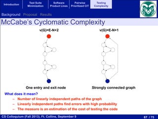
In the following paragraphs we describe the McCabe’s cyclomatic compl
measures in detail.
Halstead complexity measures are software metrics [14] introduced by
Halstead’s Metrics are based on arguments derived from common sense, i
The metrics are based on four easily measurable properties of the progra
• n1 = the number of distinct operators
• n2 = the number of distinct operands
• N1 = the total number of operators
• N2 = the total number of operands
From these values, six measures can be defined:
• Halstead Length (HL): N = N1 + N2
Legend
Background Proposal Results](https://image.slidesharecdn.com/cs-csu-chicano-140709093451-phpapp02/85/Recent-Research-in-Search-Based-Software-Testing-68-320.jpg)
![69 / 75CS Colloquium (Fall 2013), Ft. Collins, September 9
Introduction
Test Suite
Minimization
Software
Product Lines
Pairwise
Prioritized CIT
Testing
Complexity
based on the piece of code shown in Figure 1. First, we compute the
piece of code, which can be seen in Figure 2. This CFG is composed of
Bs. Interpreted as a Markov chain, the basic blocks are the states, and
robabilities to move from one basic block to another. These probabilities
d to a concrete branch. For example, to move from BB1 to BB2 in our
< 2) must be true, then according to equations (2) to (10) the probability
P(y < 2) P(x < 0) ⇤ P(y < 2) = 1
2 + 1
2
1
2 ⇤ 1
2 = 3
4 = 0.75.
/* BB1 */
if (x < 0) || (y < 2)
{
/* BB2 */
y=5;
}
else
{
/* BB3 */
x=y-3;
while (y > 5) || (x > 5)
{
/* BB4 */
y=x-5;
}
/* BB5 */
x=x-3;
}
/* BB6 */
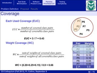
ode to illustrate the computation of Branch Coverage Expectation
transition probabilities, we build the transition matrix that represents
0
0.0 0.75 0.25 0.0 0.0 0.0
1
BB1
BB2 BB3
BB5
BB6
BB4
P(BB6,BB1)=1
P(BB2,BB6)=1
P(BB5,BB6)=1
P(BB3,BB5)=0.25
P(BB3,BB4)=0.75
P(BB4,BB4)=0.75
P(BB4,BB5)=0.25
P(BB1,BB3)=0.25
P(BB1,BB2)=0.75
Figure 2: The CFG and the probabilities used to build a Markov Chain of the piece o
exactly once the BB1 and BB6 in one run. In this way, the start and the end of t
a E[BBi] = 1. An example of the computation of the mathematical expectation is
E(BB2) = ⇡2
⇡1
= 0.1875
0.2500 = 0.75.
Table 1: Stationary probabilities and the frequency of appearance of the basic blocks of the p
Stationary Probabilities ⇡i Frequency of Appearance E
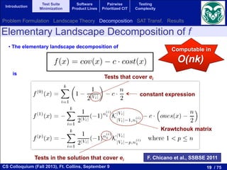
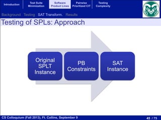
Our Proposal: Branch Coverage Expectation
P(c1&&c2) = P(c1) ⇤ P(c2), (7)
P(c1||c2) = P(c1) + P(c2) P(c1) ⇤ P(c2), (8)
P(¬c1) = 1 P(c1), (9)
P(a < b) =
1
2
, (10)
P(a b) =
1
2
, (11)
P(a > b) =
1
2
, (12)
P(a b) =
1
2
, (13)
P(a == b) = q, (14)
P(a! = b) = 1 q, (15)
where c1 and c2 are conditions.
We establish a 1/2 probability when the operators are ordering relational operators (<, , >, ). Despite
that the actual probability in a random situation is not always 1/2, we have selected the value with the
lowest error rate. In the case of equalities and inequalities the probabilities are q and 1 q, respectively,
where q is a parameter of the measure and its value should be adjusted based on the experience. Satisfying
an equality is, in general, a hard task and, thus, q should be close to zero. This parameter could be highly
dependent on the data dependencies of the program. The quality of the complexity measure depends on a
good election for q. We delay to future work the thorough analysis of this parameter. Based on a previous
phase for setting parameters, we use q = 1/16 for the experimental analysis.
Then, once we have the CFG completed with the transition probabilities, the generation of the transition
matrix is automatic. This matrix relates the states and the probability to move from one to another. We
assume, without loss of generality, that there is only one entry and exit basic block in the code. Then,
Background Proposal Results](https://image.slidesharecdn.com/cs-csu-chicano-140709093451-phpapp02/85/Recent-Research-in-Search-Based-Software-Testing-69-320.jpg)
![70 / 75CS Colloquium (Fall 2013), Ft. Collins, September 9
Introduction
Test Suite
Minimization
Software
Product Lines
Pairwise
Prioritized CIT
Testing
Complexity
BB1
BB2 BB3
BB5
BB6
BB4
P(BB6,BB1)=1
P(BB2,BB6)=1
P(BB5,BB6)=1
P(BB3,BB5)=0.25
P(BB3,BB4)=0.75
P(BB4,BB4)=0.75
P(BB4,BB5)=0.25
P(BB1,BB3)=0.25
P(BB1,BB2)=0.75
G and the probabilities used to build a Markov Chain of the piece of code of Figure 1
d BB6 in one run. In this way, the start and the end of the program always have
ple of the computation of the mathematical expectation is:
0.75.
bilities and the frequency of appearance of the basic blocks of the piece of code shown above.
Stationary Probabilities ⇡i Frequency of Appearance E[BBi]
0.2500 1.00
0.1875 0.75
0.0625 0.25
f every state in a Markov chain can be reached from every othe
hain is irreducible. For irreducible Markov chains having only p
istribution of the states q(t) tends to a given probability distributi
robability distribution ⇡ is called the stationary distribution and
near equations:
⇡T
P = ⇡T
,
⇡T
1 = 1.
.2. Definition of BCE
In our case the Markov model is built from the Control Flow G
tates of the Markov chain are the basic blocks of the program. A b
hat is executed sequentially with no interruption. It has one entry
nly the last instruction can be a jump. Whenever the first instru
est of the instructions are necessarily executed exactly once, in ord
Markov chain we must assign a value to the edges among vertic
ranches are computed according to the logical expressions that ap
efine this probability as follows:
BB1
BB2 BB3
BB5
BB6
BB4
P(BB6,BB1)=1
P(BB2,BB6)=1
P(BB5,BB6)=1
P(BB3,BB5)=0.25
P(BB3,BB4)=0.75
P(BB4,BB4)=0.75
P(BB4,BB5)=0.25
P(BB1,BB3)=0.25
P(BB1,BB2)=0.75
Figure 2: The CFG and the probabilities used to build a Markov Chain of the piece of code of Figure 1
exactly once the BB1 and BB6 in one run. In this way, the start and the end of the program always have
a E[BBi] = 1. An example of the computation of the mathematical expectation is:
E(BB2) = ⇡2
⇡1
= 0.1875
0.2500 = 0.75.
Table 1: Stationary probabilities and the frequency of appearance of the basic blocks of the piece of code shown above.
Stationary Probabilities ⇡i Frequency of Appearance E[BBi]
BB1 0.2500 1.00
BB2 0.1875 0.75
BB3 0.0625 0.25
BB4 0.1875 0.75
BB5 0.0625 0.25
BB6 0.2500 1.00
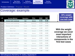
The stationary probability and the frequency of appearance of the BBs in a single execution of the piece
of code can be seen in Table 1. Now, we are able to compute the probability of appearance of a branch in
one single run. For example the expectation of traversing the branch BB3 BB4 is:
E[BB3, BB4] = E(BB3) ⇤ P34 = 1
4 ⇤ 3
4 = 3
16 = 0.1875.
In Figure 3 we show the mathematical expectations of traversing all the branches of the CFG of our
example in one single execution. So, finally we can compute the BCE by averaging the expectations of
traversing the branches which have a value lower than 1/2. We have excluded those values equals to 1/2
because both branches have the same value. In case all branches have the expectation of 1/2, then the BCE
is 1/2. In addition, a program with a Branch Coverage Expectation value of 1/2 would be the easiest one
to be tested. In this example the value of BCE is :
BCE = E[BB1,BB3]+E[BB3,BB4]+E[BB3,BB5]+E[BB4,BB5]+E[BB5,BB6]
5 =
1
4 + 3
16 + 1
16 + 3
16 + 1
4
5 = 3
16 = 0.1875.
ng parameters, we use q = 1/16 for the experiment
we have the CFG completed with the transition pr
matic. This matrix relates the states and the pro
ut loss of generality, that there is only one entry
tain a positive-recurrent irreducible Markov chain
c block (labelled as BB1) having probability 1. W
quency of appearance of each basic block in one s
y probability of a basic block is the probability of
y state. On the other hand, the frequency of appea
traversing the basic block in one single execution
E[BBi] =
⇡i
⇡1
,
mpleted with the transition probabilities, the generation of the transitio
elates the states and the probability to move from one to another. W
that there is only one entry and exit basic block in the code. Then
ent irreducible Markov chain we add a fictional link from the exit t
B1) having probability 1. We then compute the stationary probabilit
of each basic block in one single execution of the program (E[BBi]
c block is the probability of appearance in infinite program execution
hand, the frequency of appearance of a basic block is the mathematic
block in one single execution and is computed as:
E[BBi] =
⇡i
⇡1
, (16
ty of the entry basic block, BB1.
ng a branch (i, j) is computed from the frequency of appearance of th
ility to take the concrete branch from the previous basic block as:
E[BBi, BBj] = E[BBi] ⇤ Pij (17
overage Expectation (BCE) as the average of the values E[BBi, BB
Our Proposal: Branch Coverage Expectation
Markov Chain
Compute
stationary
distribution
Expected BB executions in 1 run
Expected branch execution in 1 run
Background Proposal Results](https://image.slidesharecdn.com/cs-csu-chicano-140709093451-phpapp02/85/Recent-Research-in-Search-Based-Software-Testing-70-320.jpg)
![71 / 75CS Colloquium (Fall 2013), Ft. Collins, September 9
Introduction
Test Suite
Minimization
Software
Product Lines
Pairwise
Prioritized CIT
Testing
Complexity
BCE =
1
|A|
X
(i,j)2A
E[BBi, BBj].
we analyze the new complexity measure over program artifacts,
on based on the piece of code shown in Figure 1. First, we c
his piece of code, which can be seen in Figure 2. This CFG is
BBs. Interpreted as a Markov chain, the basic blocks are the
E(BB2) = ⇡1
= 0.2500 = 0.75.
Table 1: Stationary probabilities and the frequency of appearance of the basic blocks of the piece of code shown above.
Stationary Probabilities ⇡i Frequency of Appearance E[BBi]
BB1 0.2500 1.00
BB2 0.1875 0.75
BB3 0.0625 0.25
BB4 0.1875 0.75
BB5 0.0625 0.25
BB6 0.2500 1.00
The stationary probability and the frequency of appearance of the BBs in a single execution of the pie
of code can be seen in Table 1. Now, we are able to compute the probability of appearance of a branch
one single run. For example the expectation of traversing the branch BB3 BB4 is:
E[BB3, BB4] = E(BB3) ⇤ P34 = 1
4 ⇤ 3
4 = 3
16 = 0.1875.
In Figure 3 we show the mathematical expectations of traversing all the branches of the CFG of o
example in one single execution. So, finally we can compute the BCE by averaging the expectations
traversing the branches which have a value lower than 1/2. We have excluded those values equals to 1
because both branches have the same value. In case all branches have the expectation of 1/2, then the BC
is 1/2. In addition, a program with a Branch Coverage Expectation value of 1/2 would be the easiest o
to be tested. In this example the value of BCE is :
BCE = E[BB1,BB3]+E[BB3,BB4]+E[BB3,BB5]+E[BB4,BB5]+E[BB5,BB6]
5 =
1
4 + 3
16 + 1
16 + 3
16 + 1
4
5 = 3
16 = 0.1875.
9
Our Proposal: Branch Coverage Expectation
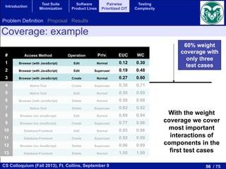
Branch Coverage Expectation
E[BBi, BBj] = E[BBi] ⇤ Pij
h Coverage Expectation (BCE) as the average of the values E[BBi
a program has a low value of BCE then a random test case gener
ber of test cases to obtain full branch coverage. The BCE is bounded
A be the set of edges with E[BBi, BBj] < 1/2:
A = {(i, j)|E[BBi, BBj] <
1
2
}.
7
Most difficult branches to cover BB1
BB2 BB3
BB5
BB6
BB4
P(BB6,BB1)=1
P(BB2,BB6)=1
P(BB5,BB6)=1
P(BB3,BB5)=0.25
P(BB3,BB4)=0.75
P(BB4,BB4)=0.75
P(BB4,BB5)=0.25
P(BB1,BB3)=0.25
P(BB1,BB2)=0.75
Figure 2: The CFG and the probabilities used to build a Markov Chain of the piece of c
exactly once the BB1 and BB6 in one run. In this way, the start and the end of the
a E[BBi] = 1. An example of the computation of the mathematical expectation is:
E(BB2) = ⇡2
⇡1
= 0.1875
0.2500 = 0.75.
Table 1: Stationary probabilities and the frequency of appearance of the basic blocks of the piec
Stationary Probabilities ⇡i Frequency of Appearance E[B
BB1 0.2500 1.00
BB2 0.1875 0.75
BB3 0.0625 0.25
Background Proposal Results](https://image.slidesharecdn.com/cs-csu-chicano-140709093451-phpapp02/85/Recent-Research-in-Search-Based-Software-Testing-71-320.jpg)
![74 / 75CS Colloquium (Fall 2013), Ft. Collins, September 9
Introduction
Test Suite
Minimization
Software
Product Lines
Pairwise
Prioritized CIT
Testing
Complexity
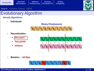
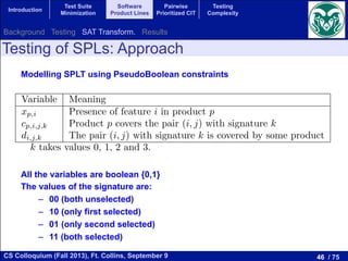
Approximated Behaviour of RND
complexity measures or other known static measures like the nesting degree.
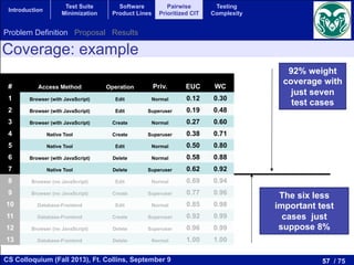
ther use of the Branch Coverage Expectation
e detailed in Section 3 for each branch (BBi, BBj) the expected number of test cases
t is 1/E[BBi, BBj]. Then, given a number of test cases x, we can compute the number
ld be theoretically traversed if the tester execute x random test cases, according to th
f(x) =
⇢
(i, j)
1
E[BBi, BBj]
< x .
ks to this estimation, we propose a theoretical prediction about the behaviour of an au
erator based on random testing.
gure 9 we show a plot for a particular program with the expected theoretical behavi
experimental data obtained using the average branch coverage of the 30 independent e
generator for that program. The features of this test program are shown in Table 9. T
how that our theoretical prediction and the experimental data are very similar. Th
n is more optimistic because it does not take into account data dependencies. At th
gorithm, the experimental behaviour is better than the theoretical prediction, but in
erage (close to 90%), the behaviour of the RND test case generator is worse than ex
on for this behaviour could be the presence of data dependencies in the program,
d in the theoretical approach in order to keep it simple.
100
his estimation, we propose a theoretical prediction about the behaviour of an automatic test
based on random testing.
we show a plot for a particular program with the expected theoretical behaviour together
mental data obtained using the average branch coverage of the 30 independent executions of
tor for that program. The features of this test program are shown in Table 9. The resulting
at our theoretical prediction and the experimental data are very similar. The theoretical
ore optimistic because it does not take into account data dependencies. At the first steps
m, the experimental behaviour is better than the theoretical prediction, but in the region of
close to 90%), the behaviour of the RND test case generator is worse than expected. One
this behaviour could be the presence of data dependencies in the program, which is not
he theoretical approach in order to keep it simple.
0 5 10 15 20 25 30
0
10
20
30
40
50
60
70
80
90
100
Number of Test Cases
BranchCoverage
Random Generator
Theoretical Prediction Approximated
number of TCs to
cover the branch
Background Proposal Results](https://image.slidesharecdn.com/cs-csu-chicano-140709093451-phpapp02/85/Recent-Research-in-Search-Based-Software-Testing-74-320.jpg)


![20260201 [FOSDEM] gomodjail - library sandboxing for Go modules.pdf](https://cdn.slidesharecdn.com/ss_thumbnails/20260201fosdemgomodjail-librarysandboxingforgomodules-260201225659-76609ec4-thumbnail.jpg?width=640&height=640&fit=bounds)


