Hey people of the world! Know what elasticity of substitution really is and find easier ways to solve such problems.

1. Elasticity of
Substitution

2. To begin with, Let’s do MRS.
 MRS or Marginal Rate of Substitution is the
number of units of Good Y to be added for
every 1 unit of Good X removed. It usually
appertains to an indifference curve of a
consumer’s utility function .
 Nevertheless, it also appertains to an isoquant
which happens to be the level curve of a
producer’s production function.
MRSXY = -∆Y/∆X

4. Elasticity of Substitution
 Let F(x,y) = c , a function of two variables, be
the function of a level curve.
 Then the slope of the level curve turns out to be
y’ = d(y)/d(x) = -F1’(x,y)/F2’(x,y). (According to
partial differentiation of implicit functions.)
 Therefore, -y’, represented by Ryx equals,
Ryx = F1’(x,y)/F2’(x,y) = MPX/MPY Or MUX/MUY
Where MP = Marginal Product and MU= Marginal Utility

5. Elasticity of Substitution
 For each value of Ryx in interval I, there
corresponds a certain point (x,y) on the level
curve F(x,y) = c, and thus a certain value of
y/x(Ryx≈-∆y/∆x).
 The fraction y/x is therefore, a function of Ryx.
 When F(x,y) = c, the elasticity of substitution
between y and x is
σyx = ElRyx(y/x)

6. IMPLICATION
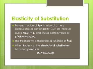
σyx = ElRyx(y/x)
 Thus, σyx is the elasticity of the fraction y/x with
respect to the marginal rate of substitution or
simply, how easy it is to substitute x for y. Roughly
speaking, it is the % change in the fraction y/x
when we move along the level curve F(x,y) = c.
 Technically speaking,
σyx = %∆(y/x)
%∆ MRSYX
 Also, σyx = -F1’F2’(xF1’+yF2’)
xy[(F2’)2
F11”-2F1’F2’F12”+(F1’)2
F22”]

7. Elucidation
 The subscript yx in RYX and MRSXY means the change
in y due to change in x. Therefore, the notation yx.
 MRSyx strictly decreases as we progress along the
level curve. For Indifference Curve, it is due to the
law of Diminishing Marginal Utility. This means that
one is willing to forgo less and less of Good X for
Good Y as one derives the maximum utility from it.
Therefore, the Indifference Curve helps solve utility
maximisation problems.
 MRSXY = MPx/MPy = -d(y)/d(x)

8. A Stimulating Problem
 Compute σyx for the Cobb-Douglas Function
Q = ALα
Kβ
(This is an isoquant level curve, since it involves labour = L and
capital = K. An isoquant curve helps with the problems of cost
minimization.)
 Before the solution, one should know that a Cobb-Douglas
Equation always has
σyx = 1
 It is known as the constant elasticity of substitution.
 General form of a Cobb-Douglas Expression is,
F(x,y) = Axa
yb

9. SolutiontotheProblem

12. Conclusion
 As we saw in the previous example,
σkl = 1
 Therefore, it is verified that a Cobb-
Douglas Function always has constant
elasticity of substitution.
 For functions in which the answer comes
with a variable, that variable tends to 0.
 For example, in σyx = 1/(1+ξ), ξ→0.

13. What do we learn
 Through this presentation, we’ve come to
know about elasticity of substitution and
how the concepts of Maths act as a
handy tool for its application.
 Also, we’re reminded of a few
rudimentary level concepts of Economics.

14. Srishti
419, 1st Year
Eco(H)