1. The document provides an introduction to using ANSYS software to perform finite element analysis (FEA). It describes the basics of solid modeling, meshing, applying loads and boundary conditions, and obtaining results in ANSYS. 2. The document then provides examples of tutorials for performing various structural and thermal analyses using the ANSYS software, including static stress analysis of plates and blocks, frame analysis with multiple materials, truss analysis, modal analysis, and buckling analysis. 3. The tutorials follow the typical ANSYS FEA procedure of preprocessing such as modeling, meshing and applying material properties; solving; and postprocessing to view and interpret results. They demonstrate how to use the various tools in ANSYS to

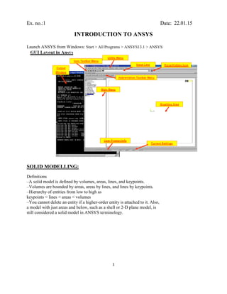
1. 1
Ex. no.:1 Date: 22.01.15
INTRODUCTION TO ANSYS
Launch ANSYS from Windows: Start > All Programs > ANSYS13.1 > ANSYS
SOLID MODELLING:
Definitions
–A solid model is defined by volumes, areas, lines, and keypoints.
–Volumes are bounded by areas, areas by lines, and lines by keypoints.
–Hierarchy of entities from low to high as
keypoints < lines < areas < volumes
–You cannot delete an entity if a higher-order entity is attached to it. Also,
a model with just areas and below, such as a shell or 2-D plane model, is
still considered a solid model in ANSYS terminology.

2. 2
METHODS OF SOLID MODELING
There are two approaches to creating a solid model in ANSYS, Top-down and Bottom-up
• Top-down modeling starts with a definition of volumes (or areas), which are then combined in
some fashion to create the final shape.
Bottom-up modeling starts with keypoints, from which you ―build up‖ lines, areas, etc.
PRIMITIVES
The volumes or areas that you initially define are called primitives, which are basic entities for
the
top-down method. ANSYS contains the following 2D and 3D primitives:

3. 3
WORK PLANE (WP)
Primitives are located and oriented with the help of the working plane. The ―WP‖ in the prompts
stands for Working Plane — a movable reference plane used to locate and orient primitives.
By default, the WP origin coincides with the global origin, but you can move it and/or rotate it to
any desired position by using following options:
Utility Menu> WorkPlane> Offset WP by increment >
Utility Menu> WorkPlane> Offset WP to >
Utility Menu> WorkPlane> Align WP with> XYZ Locations >
BOOLEAN OPERATIONS
The final shape of an object is usually not as simple as primitives. However,
it is likely doable to combine a number of primitives through a series of
proper Boolean operations. The ―input‖ to Boolean operations can be any
geometric entity, ranging from simple primitives to complicated volumes
generated in previous steps.
Boolean operations are computations involving combinations of geometric
entities. ANSYS Boolean operations include add, subtract, intersect, divide,
glue, and overlap. •All Boolean operations are available in the GUI:
Main Menu > Preprocessor > Modeling > Operate > Booleans
By default, input entities of a Boolean operation are deleted after the
operation.

4. 4
Add: Combines two or more entities into one.
Glue: Attaches two or more entities by creating a common
boundary between them, which is useful when you want to
maintain the distinction between entities (such as for different
materials).
Overlap: Same as glue, except that the input entities overlap
each other.
Subtract: Removes the overlapping portion of one or more

5. 5
entities from a set of ―base‖ entities, which can be useful for
creating holes or trimming off portions of an entity.
Divide: Cuts an entity into two or more pieces that are still
connected to each other by common boundaries. The ―cutting
tool‖ may be the working plane, an area, a line, or even a
volume. Useful for ―slicing and dicing‖ a complicated
volume into simpler volumes for brick meshing.
Intersect: Keeps only the overlapping portion of two or more
entities.
Partition: Cuts two or more intersecting entities into multiple

6. 6
pieces that are still connected to each other by common
boundaries, e.g., to find the intersection point of two lines and still
retain all four line segments, as shown. (An intersection operation
would return the common keypoint and delete both lines.)
FINITE ELEMENT DISCRETISATION
Finite Element Discretization or Meshing is the process used to ―fill‖ the solid model with nodes
and elements, i.e, to create the FEA model. Remember, you need nodes and elements for the
finite element solution, not just the solid model. The Solid Model in CAD does NOT participate
in the
finite element solution.
ELEMENT TYPE
The element type is an important choice that determines the following element characteristics:
• Degree of Freedom (DOF) set. A thermal element type, for example, has one dof: TEMP,
whereas a structural element type may have up to six dof: UX, UY, UZ, ROTX, ROTY, ROTZ.
• Element shape -- brick, tetrahedron, quadrilateral, triangle, etc.
• Dimensionality -- 2-D solid (X-Y plane only), or 3-D solid.
• Assumed displacement shape -- linear vs. quadratic.
To define an element:
Main Menu>Preprocessor>Element Type> Add/Edit/Delete>Add

7. 7
MESHING METHODS :There are two main meshing methods: free and mapped.
Free Mesh–Has no element shape restrictions.
–The mesh does not follow any pattern.
–Suitable for complex shaped areas and volumes.
–Suitable for complex shaped areas and volumes.
–Volume meshes consist of high order tetrahedral (10 nodes), large dof.
Mapped Mesh–Restricts element shapes to quadrilaterals (areas) and hexahedra
(volume)
–Typically has a regular pattern with obvious rows of elements.
–Suitable only for ―regular‖ shapes such as rectangles and bricks.
Mesh Density Control
ANSYS provides many tools to control mesh density, on a global and local level:
–Global controls: SmartSizing; Global element sizing; Default sizing
6
–Local controls: Keypoint sizing; Line sizing; Area sizing
To bring up the MeshTool:
Main Menu > Preprocessor > Meshing > MeshTool
SmartSizing: by turning on SmartSizing, and set the desired size level. Size level ranges from 1
(fine) to 10 (coarse), defaults to 6. Then mesh all volumes (or all areas) at once, rather than one-
byone.
Advanced SmartSize controls, such as mesh expansion and transition factors, are available by
Main Menu>Preprocessor>Meshing>Size Cntrls>SmartSize>Adv Opts
Global Element Sizing: Allows you to specify a maximum element edge length for the entire
model (or number of divisions per line):
Go to ―Size Controls‖, ―Global‖ ,and click [Set] or
Main Menu>Preprocessor>Meshing>Size Cntrls>ManualSize>Global >Size

8. 8
Material Properties
Every analysis requires some material property input: Young‘s modulus (EX), Poisson‘s ratio
(PRXY) for structural elements, thermal conductivity (KXX) for thermal elements, etc.
To define the material properties:
Main Menu>Preprocessor>Material Props>Material Models
ANSYS FEA PROCEDURE
In general, a finite element solution may be broken into the following three stages.
• Preprocessing: defining the problem; the major steps in preprocessing are given below:
Define keypoints/lines/areas/volumes (Solid Modeling)
Define element type and material/geometric properties
Mesh lines/areas/volumes as required
• Solution: assigning loads, constraints and solving;
Apply the loads (point or pressure), Specify constraints (translational and rotational)
Finally solve the problem.
• Postprocessing: further processing and viewing of the results;
Lists of nodal displacements and show the deformation
Element forces and moments
Stress/strain contour diagrams

9. 9
Ex. no.:2 Date: 29.01.15
2 DIMENSIONAL STATIC STRESS ANALYSIS IN RECTANGULAR
PLATE
AIM:
Determine the stress concentration in a rectangular plate of length 50cm and width 20cm
with hollow circles at the centre. Load on right edge of the rectangular plate is 10x105
N.
Young‘s modulus of 70E9
N/cm2
and of Poission ratio 0.3
SYSTEM CONFIGURATION:
ANSYS Version 12.1
17‖ VGA color Monitor
Intel I3 processor
320 GB HDD
2GB RAM
ANSYS PROCEDURE:
Preference Structural
Preprocessor elemental type addaddSolidQuad 4node 42OK
Material properties  Material Models  Structural  Linear 
Elastic  isotropic (enter Young‘s Modulus Value & Possion Ratio)
modelingcreatearearectangleby dimensions
enter the lower left coordinates(X,Y),the width and height
meshingmesh toolmeshareapick area
loadsnew analysisanalysis typestatic
applyloadsdisplacementUxOK
applypressureon linesOK
Solution solvecurrent LS
General

10. 10
post processorplot results nodal solutionsDOF solutions vector sum plot
list resultsnodal solutionsDOF solutions vector sum plot
RESULTS
Original and deformed shape of 2D plane
Stress distribution of 2D plane

11. 11
Ex. no.:3 Date: 05.02.15
3 DIMENSIONAL STATIC STRESS ANALYSIS IN BLOCK
AIM:
Determine the stress concentration in a large isotropic block subjected to a point
load of 22500 N downward and fixed at the bottom.Youngs modulus 144e7
N/mm2
,
Poisson ratio 0.34
SYSTEM CONFIGURATION:
ANSYS Version 12.1
17‖ VGA color Monitor
Intel I3 processor
320 GB HDD
2GB RAM
ANSYS PROCEDURE:
Preference Structural
Preprocessor elemental type addaddSolidbrick 8 node 45OK
Material properties  Material Models  Structural  Linear
 Elastic  isotropic (enter Young‘s Modulus Value & Poisson Ratio)
Modelingcreatevolumesblockby dimensions
Enter the coordinates(X, Y)
Meshingmesh toolmeshvolumepick volume
Loadsnew analysisanalysis typestatic
Applyloadsdisplacementall DOFOK
Applyforce and momenton nodeOK
Solution solvecurrent LS
General
Post processorplot results nodal solutionsDOF solutions vector sum plot

12. 12
List resultsnodal solutionsDOF solutions vector sum plot
RESULTS
Original and deformed shape of 3D volume
Stress distribution of 3D volume

13. 13
Ex. no.:4 Date: 12.02.15
2 DIMENSIONAL FRAME WITH MULTIPLE MATERIALS AND
ELEMENT TYPE ANALYSIS
AIM:
Determine the stress concentration in 2D frame with multiple materials and
element type analysis.Young‘s modulus of 70E9 N/cm2
and of Poisson ratio 0.3.
SYSTEM CONFIGURATION:
ANSYS Version 12.1
17‖ VGA color Monitor
Intel I3 processor
320 GB HDD
2GB RAM
ANSYS PROCEDURE:
Preference Structural
Preprocessor elemental type addaddLink3D finite stn 180
Material properties  Material Models  Structural  Linear 
Elastic  isotropic (enter Young‘s Modulus Value & Possion Ratio)
modelingcreatekeypointsby dimensions
lineslinesstraight linesjoin keypoints
meshingmesh toolmeshlinepick lines
loadsnew analysisanalysis typestatic
applyloadsdisplacementUxOK
applypressureon linesOK
Solution solvecurrent LS
General
post processorplot results nodal solutionsDOF solutions vector sum plot

14. 14
list resultsnodal solutionsDOF solutions vector sum plot
RESULTS
Original and deformed shape of multi frame
Stress distribution of multi frame

15. 15
Ex. No.:5 Date: 19.02.15
3 DIMENSIONAL TRUSS ANALYSIS
AIM:
Determine the stress concentration in 3D truss. Young‘s modulus of 70E9
N/cm2
and of Poission ratio 0.3
SYSTEM CONFIGURATION:
ANSYS Version 12.1
17‖ VGA color Monitor
Intel I3 processor
320 GB HDD
2GB RAM
ANSYS PROCEDURE:
Preference Structural
Preprocessor elemental type addaddlink3D finite stn 180 OK
Material properties  Material Models  Structural  Linear 
Elastic  isotropic (enter Young‘s Modulus Value & Possion Ratio)
modelingcreatekeypoints
lineslinesstraight line join key points
meshingmesh toollinesmeshpick lines
loadsnew analysisanalysis typestatic
applyloadsdisplacementUxOK
applyforce and momentson nodesOK
Solution solvecurrent LS
General
post processorplot results nodal solutionsDOF solutions vector sum plot
list resultsnodal solutionsDOF solutions vector sum plot

16. 16
RESULTS
Original and deformed shape of 3D truss
Stress distribution of 3D truss

17. 17
Ex. No.:6 Date: 26.02.15
MODAL ANALYSIS IN ANSYS
AIM:
Determine the first five modal natural frequency of square plate of area 1m2
. Young‘s
modulus of 70E9
N/cm2
, Poission ratio of 0.3 and density 2.7E3
.
SYSTEM CONFIGURATION:
ANSYS Version 12.1
17‖ VGA color Monitor
Intel I3 processor
320 GB HDD
2GB RAM
ANSYS PROCEDURE:
Preference Structural
Preprocessor elemental type addaddsolidquad 4 node 182 OK
Material properties  Material Models  Structural  Linear 
Elastic  isotropic (enter Young‘s Modulus Value & Possion Ratio)
modelingcreatearearectangleby dimensions
circleby dimensions
operatebooleanssubtractareas
meshingmesh toolareasmeshpick areas
loadsapplyloadsdisplacementUx(upper edge & bottom
edge)OK
 applyloadsdisplacementUy(left edge & right edge)OK
Solution analysis typenew analysismodal
analysis optionsenter no. Modes:5
enter no. of mode expansions:5

18. 18
solvecurrent LS
General
post processorread results first set
list resultsnodal solutionsDOF solutions vector sum plot
 plot results nodal solutionsDOF solutions vector sum plot
RESULTS
Modal frequencies for 5 modes of 2D plane
SET TIME/FREQ LOAD STEP SUBSTEP CUMULATIVE
1 2289.8 1 1 1
2 2853.0 1 2 2
3 2853.7 1 3 3
4 3379.7 1 4 4
5 4067.9 1 5 5
Modal Displacement distribution of 2D plane

19. 19
Ex. No.:7 Date: 05.03.15
PLATE BUCKING ANALYSIS EIGEN BUCKLING ANALYSIS
AIM:
Determine the plate bucking analysis Eigen buckling analysis of rectangular plate of
width 10cm and height 0f 2cm.Young‘s modulus of 70E9
N/cm2
, Poission ratio of 0.3 and
density 2.7E3
.
SYSTEM CONFIGURATION:
ANSYS Version 12.1
17‖ VGA color Monitor
Intel I3 processor
320 GB HDD
2GB RAM
ANSYS PROCEDURE:
Preference Structural
Preprocessor elemental type addaddsolidquad 4 node 182 OK
Material properties  Material Models  Structural  Linear 
Elastic  isotropic (enter Young‘s Modulus Value & Possion Ratio)
modelingcreatearearectangleby dimensions
meshingmesh toolareasmeshpick areas
loadsapplyloadsdisplacementUx(left edge),Uy(bottom)OK
applyloadspressureon lines(right edge line)enter the
pressure value
Solution analysis typenew analysisstatic
analysis optionsenter no. Modes:5
enter no. of mode expansions:5

20. 20
solvecurrent LS
General
post processorread results first set
list resultsnodal solutionsDOF solutions vector sum plot
 plot results nodal solutionsDOF solutions vector sum plot
RESULTS:
Bucking mode values:
SET TIME/FREQ LOAD STEP SUBSTEP CUMULATIVE
1 0.77570E+08 1 1 1
2 0.10039E+09 1 2 2
3 0.11611E+09 1 3 3
4 0.11734E+09 1 4 4
5 0.11930E+09 1 5 5

21. 21
Original and buckled deformation
Displacement distribution of buckled deformation

22. 22
Ex. No.:8 Date: 12.03.15
SIMPLE DYNAMIC ANALYSIS
AIM:
Determine the plate bucking analysis Eigen buckling analysis of rectangular plate of
width 10cm and height 0f 2cm.Young‘s modulus of 70E9
N/cm2
, Poission ratio of 0.3 and
density 2.7E3
.
SYSTEM CONFIGURATION:
ANSYS Version 12.1
17‖ VGA color Monitor
Intel I3 processor
320 GB HDD
2GB RAM
ANSYS PROCEDURE:
Preference Structural
Preprocessor elemental type addaddsolidquad 4 node 182 OK
Material properties  Material Models  Structural  Linear 
Elastic  isotropic (enter Young‘s Modulus Value & Possion Ratio)
modelingcreatearearectangleby dimensions
meshingmesh toolareasmeshpick areas
loadsapplyloadsdisplacementUx(left edge),Uy(bottom)OK
applyloadspressureon lines(right edge line)enter the
pressure value
Solution analysis typenew analysisstatic
analysis optionsenter no. Modes:5
enter no. of mode expansions:5

23. 23
solvecurrent LS
General
post processorread results first set
list resultsnodal solutionsDOF solutions vector sum plot
 plot results nodal solutionsDOF solutions vector sum plot
RESULTS:
Dynamic 4 step load data:
SET TIME/FREQ LOAD STEP SUBSTEP CUMULATIVE
1 0.10000E-04 1 10 10
2 0.50000E-04 2 8 18
3 0.60000E-04 3 10 28
4 0.60000E-01 4 100 128
Time history deflection graph

24. 24
Ex. no.:9 Date: 19.03.15
BOX BEAM ANALYSIS
AIM:
Determine the stress concentration and displacement in box beam materials.
Young‘s modulus of 70E9 N/cm2
and of Poisson ratio 0.3.
SYSTEM CONFIGURATION:
ANSYS Version 12.1
17‖ VGA color Monitor
Intel I3 processor
320 GB HDD
2GB RAM
ANSYS PROCEDURE:
Preference Structural
Preprocessor elemental type addaddbeam2 Node 188
Material properties  Material Models  Structural  Linear 
Elastic  isotropic (enter Young‘s Modulus Value & Possion Ratio)
modelingcreatenodesby dimensions
Elementsthrough nodesjoin nodes
loadsnew analysisanalysis typestatic
applyloadsdisplacementall dof at left edgeOK
applyforce and momenton nodeOK
Solution solvecurrent LS
General
post processorplot results nodal solutionsDOF solutions vector sum plot
list resultsnodal solutionsDOF solutions vector sum plot

25. 25
RESULTS:
Original and deformed box beam
Stress concentration in box beam

26. 26
Ex. no.:10 Date: 26.03.15
STEADY STATE HEAT CONDUCTION IN SOLIDS
AIM:
Determine the temperature distribution in a square plate of side 1m and thichness1m with
thermal conductivity k1=25 W/m 0
C,k2= 50 W/m 0
C ,k3=30 W/m 0
C.The convection takes place
on the right edge of the plate with free stream temperature of 50 0
C.The left edge of the plate is
maintained at a temperature of 100 0
C and the top and bottom edges are insulated.
SYSTEM CONFIGURATION:
ANSYS Version 12.1
17‖ VGA color Monitor
Intel I3 processor
320 GB HDD
2GB RAM
ANSYS PROCEDURE
Preference thermal
Preprocessor elemental type addaddthermal massbrick 20 node 90
material propertiesisotropic(enter thermal conductivity value K)
modelingcreatearearectangleby two corners
enter the lower left coordinates(X,Y),the width and height
meshingsize controlmanual sizeglobalsize
element edge length
meshareapick area
loadsnew analysisanalysis typesteady state
applytemperatureon linepick the top edgeapply
(enter the temperature value)
applyheat fluxon linepick the right, left and bottom edge.

27. 27
apply (enter heat flux value as 0)
heat generation on area pick all ok
Solution solvecurrent LS
General
post processorplot results nodal solutionsDOF solutions temperature
list resultsnodal solutionsDOF solutions temperature

28. 28
RESULTS:
Temperature distribution
Vector plot of temperature distribution

29. 29
Ex. no.:11 Date: 26.03.15
STEADY STATE HEAT CONVECTION IN SOLIDS
AIM :
Determine the temperature distribution in a square plate of side 2m and thichness1m with
thermal conductivity K=25 W/m 0
C and convection film co-efficient h=20 W/m2 0
C.The
convection takes place on the right edge of the plate with free stream temperature of 50 0
C.The
left edge of the plate is maintained at a temperature of 100 0
C and the top and bottom edges are
insulated.
SYSTEM CONFIGURATION :
ANSYS Version 12.1
17‖ VGA color Monitor
Intel I3 processor
320 GB HDD
2GB RAM
ANSYS PROCEDURE :
Preference thermal
Preprocessor elemental type addaddthermal massbrick 20 node 90
material propertiesisotropic(enter thermal conductivity value K)
modelingcreatearearectangleby two corners
enter the lower left coordinates(X,Y),the width and height
meshingsize controlmanual sizeglobalsize
element edge length
meshareapick area
loadsnew analysisanalysis typesteady state
applytemperatureon linepick the top edgeapply
(enter the temperature value)

30. 30
applyheat fluxon linepick the right, left and bottom edge.
apply (enter heat flux value as 0)
heat generation on area pick all ok
Solution solvecurrent LS
General
post processorplot results nodal solutionsDOF solutions temperature
list resultsnodal solutionsDOF solutions temperature

31. 31
RESULTS:
Temperature distribution by convection
‗
Vector plot of temperature

32. 32
Ex. no.:12 Date: 02.04.15
STEADY STATE RADIATIVE HEAT TRANSFER
AIM:
Determine the temperature distribution in a square plate of side 2m and thickness
1m with Thermal conductivity K = 25W/mo
C and Boltzmann Constant σ = 5.67x10-8
W m-2
K-
4
. The Radiation takes place on the right edge of the plate with free stream temperature of 50o
c.
The left edge of the plate is maintained at a temperature of 100o
c and the top and bottom edge
are insulated.
SYSTEM CONFIGURATION:
ANSYS Version 12.1
17‖ VGA Color monitor
Intel I3 Processor
320 GB HDD
2 GB RAM
ANSYS PROCEDURE :
Preference thermal
Preprocessor elemental type addaddthermal massbrick 20 node 90
material propertiesisotropic(enter thermal conductivity value K)
modelingcreatearearectangleby two corners
enter the lower left coordinates(X,Y),the width and height
meshingsize controlmanual sizeglobalsize
element edge length
meshareapick area
loadsnew analysisanalysis typesteady state
applytemperatureon linepick the top edgeapply
(enter the temperature value)

33. 33
Radiation  Solution Options( enter the Boltzmann Constant, σ = 5.67x10-8
W m-2
K-4
)
Option
applyheat fluxon linepick the right, left and bottom edge.
apply (enter heat flux value as 0)
heat generation on area pick all ok
Solution solvecurrent LS
General
post processorplot results nodal solutionsDOF solutions temperature
listresultsnodalsolutionsDOFsolutionstemperature

34. 34
RESULTS:
Temperature distribution by radiation
Vector plot of temperature distribution

35. 35
Ex. no.:13 Date: 09.04.15
COMBINED CONDUCTION AND CONVECTION HEAT HEAT
TRANSFER ANALYSIS
AIM :
Determine the temperature distribution in a square plate of side 2m and thichness1m with
thermal conductivity K=25 W/m 0
C and convection film co-efficient h=20 W/m2 0
C.The
convection takes place on the right edge of the plate with free stream temperature of 50 0
C.The
left edge of the plate is maintained at a temperature of 100 0
C and the top and bottom edges are
insulated.
SYSTEM CONFIGURATION :
ANSYS Version 12.1
17‖ VGA color Monitor
Intel I3 processor
320 GB HDD
2GB RAM
ANSYS PROCEDURE
Preference thermal
Preprocessor elemental type addaddthermal massbrick 20 node 90
material propertiesisotropic(enter thermal conductivity value K)
modelingcreatearearectangleby two corners
enter the lower left coordinates(X,Y),the width and height
meshingsize controlmanual sizeglobalsize
element edge length
meshareapick area
loadsnew analysisanalysis typesteady state
applytemperatureon linepick the top edgeapply

36. 36
(enter the temperature value)
applyheat fluxon linepick the right, left and bottom edge.
apply (enter heat flux value as 0)
heat generation on area pick all ok
Solution solvecurrent LS
General
post processorplot results nodal solutionsDOF solutions temperature
list resultsnodal solutionsDOF solutions temperature

37. 37
RESULTS:
Temperature distribution with combined conduction and convection
.
Vector plot of temperature distribution

38. 38
Ex. no.:14 Date: 09.04.15
COMBINED CONDUCTION AND RADIATION HEAT TRANSFER
ANALYSIS
AIM:
Determine the temperature distribution in a square plate of side 2m and thickness 1m
with thermal conductivity K=25 W/m 0
C and Boltzmann‘s constant (σ)= 5.67*10-8
W.m-2
.k-4
.The
radiation takes place on the right edge of the plate with free stream temperature of 50 0
C. The left
edge of the plate is maintained at a temperature of 100 0
C.
SYSTEM CONFIGURATION:
ANSYS Version 12.1
17‖ VGA color Monitor
Intel I3 processor
320 GB HDD
2GB RAM
ANSYS PROCEDURE :
Preferencethermal
Preprocessorelemental type addaddthermal massbrick 20 node 90
material propertiesisotropic(enter thermal conductivity value K)
modelingcreatearearectangleby two corners
enter the lower left coordinates(X,Y),the width and height
meshingsize controlmanual sizeglobalsize
element edge length
meshareapick area
loadsnew analysisanalysis typesteady state
applytemperatureon linepick the top edgeapply

39. 39
(enter the temperature value)
Radiation optionssolution optionsBoltzmann‘s constant(σ)= 5.67*10-8
W.m-2
.k-4
applyheat fluxon linepick the right, left and bottom edge.
apply (enter heat flux value as 0)
heat generation on area pick all ok
Solutionsolvecurrent LS
General post processorplot results nodal solutionsDOF solutions temperature
list resultsnodal solutionsDOF solutions temperature

40. 40
RESULTS:
Temperature distribution with combined conduction and radiation
Vector plot of temperature distribution

41. 41
Ex. no.:15 Date: 16.04.15
COMBINED CONVECTION AND RADIATION HEAT TRANSFER IN
CYLINDER
AIM:
Determine the temperature distribution in a cylinder of radius 2m and thickness 10m with
thermal conductivity K=25 W/m 0
C and radiation Boltzman‘s constant =5.67^10
-8
W/m-2
K-4
.
The convection and radiation takes place on the right edge of the cylinder with free stream
temperature of 50 0
C.The left edge of the plate is maintained at a temperature of 100 0
C.
SYSTEM CONFIGURATION:
ANSYS Version 12.1
17‖ VGA color Monitor
Intel I3 processor
320 GB HDD
2GB RAM
ANSYS PROCEDURE:
Preference thermal
Preprocessor elemental type addaddthermal massbrick 20 node 90
material propertiesisotropic(enter thermal conductivity value K)
modelingcreatearearectangleby two corners
enter the lower left coordinates(X,Y),the width and height
meshingsize controlmanual sizeglobalsize
element edge length
meshareapick area
loadsnew analysisanalysis typesteady state
applytemperatureon linepick the top edgeapply
(enter the temperature value)

42. 42
radiation options solution options Stefen-Boltzman’s
constant=5.67^10
-8
W/m-2
K-4
applyheat fluxon linepick the right, left and bottom edge.
apply (enter heat flux value as 0)
heat generation on area pick all ok
Solution solvecurrent LS
General
post processorplot results nodal solutionsDOF solutions temperature
list resultsnodal solutionsDOF solutions temperature

43. 43
RESULTS:
Temperature distribution with combined convection and radiation
Vector plot of temperature distribution

44. 44
Ex. no.:16 Date: 23.04.15
UNSTEADY STATE CONDUCTION AND CONVECTION HEAT
TRANSFER IN SQUARE PLATE
AIM :
Determine the temperature distribution in a square plate of side 2m and thichness1m with
thermal conductivity K=25 W/m 0
C and convection film co-efficient h=20 W/m2 0
C.The
convection takes place on the right edge of the plate with free stream temperature of 50 0
C.The
left edge of the plate is maintained at a temperature of 100 0
C and the top and bottom edges are
insulated.
SYSTEM CONFIGURATION :
ANSYS Version 12.1
17‖ VGA color Monitor
Intel I3 processor
320 GB HDD
2GB RAM
ANSYS PROCEDURE:
Preference thermal
Preprocessor elemental type addaddthermal massbrick 20 node 90
material propertiesisotropic(enter thermal conductivity value K)
modelingcreatearearectangleby two corners
enter the lower left coordinates(X,Y),the width and height
meshingsize controlmanual sizeglobalsize
element edge length
meshareapick area
loadsnew analysisanalysis typesteady state
applytemperatureon linepick the top edgeapply
(enter the temperature value)

45. 45
applyheat fluxon linepick the right, left and bottom edge.
apply (enter heat flux value as 0)
heat generation on area pick all ok
Solution solvecurrent LS
General
post processorplot results nodal solutionsDOF solutions temperature
list resultsnodal solutionsDOF solutions temperature

46. 46
RESULTS:
Unsteady Temperature distribution with combined conduction and convection
Vector plot of unsteady temperature distribution

47. 47
Ex. no.:17 Date: 30.04.15
UNSTEADY STATE CONDUCTION AND RADIATION HEAT
TRANSFER ANALYSIS
AIM:
Determine the temperature distribution in a square plate of side 2m and thickness 1m
with thermal conductivity K=25 W/m 0
C and Boltzmann‘s constant (σ)= 5.67*10-8
W.m-2
.k-4
.The
radiation takes place on the right edge of the plate with free stream temperature of 50 0
C. The left
edge of the plate is maintained at a temperature of 100 0
C.
SYSTEM CONFIGURATION:
ANSYS Version 12.1
17‖ VGA color Monitor
Intel I3 processor
320 GB HDD
2GB RAM
ANSYS PROCEDURE
Preferencethermal
Preprocessorelemental type addaddthermal massbrick 20 node 90
material propertiesisotropic(enter thermal conductivity value K)
modelingcreatearearectangleby two corners
enter the lower left coordinates(X,Y),the width and height
meshingsize controlmanual sizeglobalsize
element edge length
meshareapick area
loadsnew analysisanalysis typesteady state
applytemperatureon linepick the top edgeapply

48. 48
(enter the temperature value)
Radiation optionssolution optionsBoltzmann‘s constant(σ)= 5.67*10-8
W.m-2
.k-4
applyheat fluxon linepick the right, left and bottom edge.
apply (enter heat flux value as 0)
heat generation on area pick all ok
Solutionsolvecurrent LS
General post processorplot results nodal solutionsDOF solutions temperature
list resultsnodal solutionsDOF solutions temperature

49. 49
RESULTS:
Unsteady Temperature distribution with combined conduction and radiation
Vector plot of unsteady temperature distribution