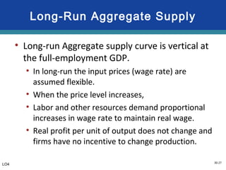
Potential GDP
0
ASLR1
ASLR2
Long-run aggregate supply increases when productivity or the quantity of resources increases permanently. This shifts the long-run aggregate supply curve rightward, increasing the potential GDP of the economy.
30-2
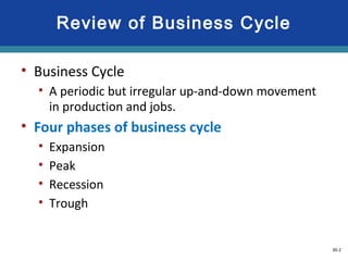
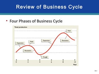
Review of BusinessCycle
• Business Cycle
• A periodic but irregular up-and-down movement
in production and jobs.
• Four phases of business cycle
• Expansion
• Peak
• Recession
• Trough
30-4
Overview of AD-ASModel
• Aggregate Demand and Aggregate Supply Model
• The aggregate demand (AD) and aggregate supply
(AS) model shows a relationship between the
price level in an economy and the real GDP of the
economy.
• Three components of the AD-AS model
• Aggregate demand
• Aggregate supply
• Potential GDP (Long-run Aggregate supply)
5.
30-5
Overview of AD-ASModel
• Potential GDP is determined by the economy’s
production capacity.
• Aggregate supply comes from the economy’s
production decisions by firms.
• Aggregate demand comes from the economy’s
expenditure decisions by households, firms,
governments, and foreigners.
• These three components determine a
macroeconomic equilibrium.
6.
30-6
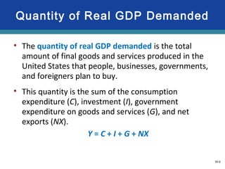
• The quantityof real GDP demanded is the total
amount of final goods and services produced in the
United States that people, businesses, governments,
and foreigners plan to buy.
• This quantity is the sum of the consumption
expenditure (C), investment (I), government
expenditure on goods and services (G), and net
exports (NX).
Y = C + I + G + NX
Quantity of Real GDP Demanded
7.
30-7
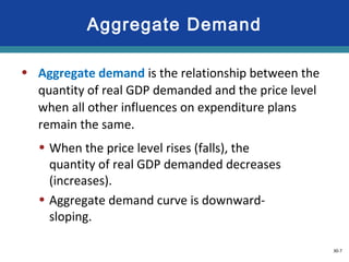
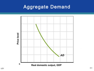
• Aggregate demandis the relationship between the
quantity of real GDP demanded and the price level
when all other influences on expenditure plans
remain the same.
• When the price level rises (falls), the
quantity of real GDP demanded decreases
(increases).
• Aggregate demand curve is downward-
sloping.
Aggregate Demand
8.
30-8
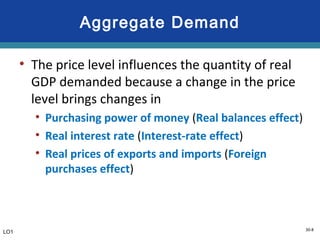
Aggregate Demand
• Theprice level influences the quantity of real
GDP demanded because a change in the price
level brings changes in
• Purchasing power of money (Real balances effect)
• Real interest rate (Interest-rate effect)
• Real prices of exports and imports (Foreign
purchases effect)
LO1
30-10
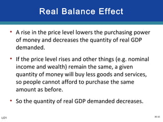
Real Balance Effect
•A rise in the price level lowers the purchasing power
of money and decreases the quantity of real GDP
demanded.
• If the price level rises and other things (e.g. nominal
income and wealth) remain the same, a given
quantity of money will buy less goods and services,
so people cannot afford to purchase the same
amount as before.
• So the quantity of real GDP demanded decreases.
LO1
11.
30-11
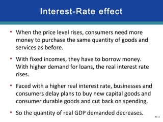
Interest-Rate effect
• Whenthe price level rises, consumers need more
money to purchase the same quantity of goods and
services as before.
• With fixed incomes, they have to borrow money.
With higher demand for loans, the real interest rate
rises.
• Faced with a higher real interest rate, businesses and
consumers delay plans to buy new capital goods and
consumer durable goods and cut back on spending.
• So the quantity of real GDP demanded decreases.
12.
30-12
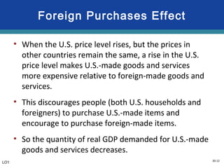
Foreign Purchases Effect
•When the U.S. price level rises, but the prices in
other countries remain the same, a rise in the U.S.
price level makes U.S.-made goods and services
more expensive relative to foreign-made goods and
services.
• This discourages people (both U.S. households and
foreigners) to purchase U.S.-made items and
encourage to purchase foreign-made items.
• So the quantity of real GDP demanded for U.S.-made
goods and services decreases.
LO1
13.
30-13
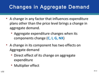
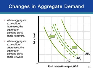
Changes in AggregateDemand
• A change in any factor that influences expenditure
plans other than the price level brings a change in
aggregate demand.
• Aggregate expenditure changes when its
components change (C, I, G, NX)
• A change in its component has two effects on
Aggregate demand
• Direct effect of its change on aggregate
expenditure
• Multiplier effect
LO2
14.
30-14
Changes in AggregateDemand
Real domestic output, GDP
Pricelevel
AD1
AD3
AD2
0
• When aggregate
expenditure
increases, the
aggregate
demand curve
shifts rightward.
• When aggregate
expenditure
decreases, the
aggregate
demand curve
shifts leftward.
30-16
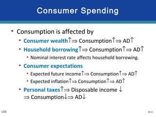
Investment Spending
• Investmentspending is affected by
• Real interest rates↑⇒ Investment↓⇒ AD↓
• Expected returns↑⇒ Investment↑⇒ AD↑
• Expected returns ↑ when
• Expectations about future business conditions ↑
• Technology ↑
• Degree of excess capacity↓
• Business taxes ↓
LO2
17.
30-17
Government Spending
• Aggregatedemand increases when
• Government spending increases
• Increased spending on infrastructure (highways, ports,
public utility), military, and education
• Transfer payments increases
• Extended unemployment benefits, increased welfare
benefits, increased social security
• Taxes decreases (through consumption and
investment)
• Income tax return, payroll tax reduction
LO2
18.
30-18
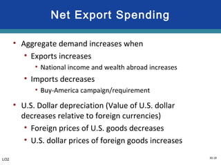
Net Export Spending
•Aggregate demand increases when
• Exports increases
• National income and wealth abroad increases
• Imports decreases
• Buy-America campaign/requirement
• U.S. Dollar depreciation (Value of U.S. dollar
decreases relative to foreign currencies)
• Foreign prices of U.S. goods decreases
• U.S. dollar prices of foreign goods increases
LO2
19.
30-19
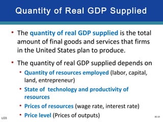
Quantity of RealGDP Supplied
• The quantity of real GDP supplied is the total
amount of final goods and services that firms
in the United States plan to produce.
• The quantity of real GDP supplied depends on
• Quantity of resources employed (labor, capital,
land, entrepreneur)
• State of technology and productivity of
resources
• Prices of resources (wage rate, interest rate)
• Price level (Prices of outputs)LO3
20.
30-20
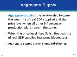
Aggregate Supply
• Aggregatesupply is the relationship between
the quantity of real GDP supplied and the
price level when all other influences on
production plans remain the same.
• When the price level rises (falls), the quantity
of real GDP supplied increases (decreases).
• Aggregate supply curve is upward-sloping.
LO3
21.
30-21
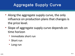
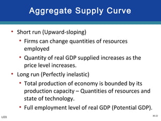
Aggregate Supply Curve
•Along the aggregate supply curve, the only
influence on production plans that changes is
the price level.
• Slope of aggregate supply curve depends on
time horizon
• Immediate short run
• Short run
• Long run
LO3
22.
30-22
Aggregate Supply Curve
•Short run (Upward-sloping)
• Firms can change quantities of resources
employed
• Quantity of real GDP supplied increases as the
price level increases.
• Long run (Perfectly inelastic)
• Total production of economy is bounded by its
production capacity – Quantities of resources and
state of technology.
• Full employment level of real GDP (Potential GDP).
LO3
30-24
Aggregate Supply: LongRun
Real GDP
Pricelevel
ASLR
Qf (Full-employment GDP)0
Long-run
aggregate
supply
LO3
25.
30-25
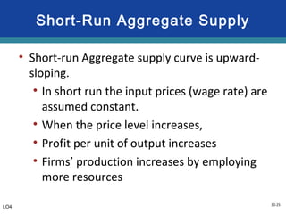
Short-Run Aggregate Supply
•Short-run Aggregate supply curve is upward-
sloping.
• In short run the input prices (wage rate) are
assumed constant.
• When the price level increases,
• Profit per unit of output increases
• Firms’ production increases by employing
more resources
LO4
26.
30-26
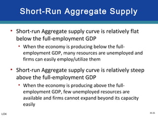
Short-Run Aggregate Supply
•Short-run Aggregate supply curve is relatively flat
below the full-employment GDP
• When the economy is producing below the full-
employment GDP, many resources are unemployed and
firms can easily employ/utilize them
• Short-run Aggregate supply curve is relatively steep
above the full-employment GDP
• When the economy is producing above the full-
employment GDP, few unemployed resources are
available and firms cannot expand beyond its capacity
easily
LO4
27.
30-27
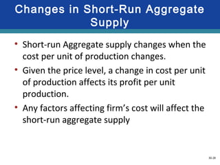
Long-Run Aggregate Supply
•Long-run Aggregate supply curve is vertical at
the full-employment GDP.
• In long-run the input prices (wage rate) are
assumed flexible.
• When the price level increases,
• Labor and other resources demand proportional
increases in wage rate to maintain real wage.
• Real profit per unit of output does not change and
firms have no incentive to change production.
LO4
28.
30-28
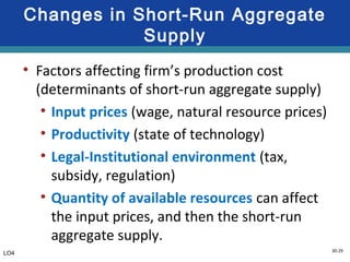
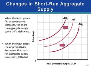
Changes in Short-RunAggregate
Supply
• Short-run Aggregate supply changes when the
cost per unit of production changes.
• Given the price level, a change in cost per unit
of production affects its profit per unit
production.
• Any factors affecting firm’s cost will affect the
short-run aggregate supply
29.
30-29
Changes in Short-RunAggregate
Supply
• Factors affecting firm’s production cost
(determinants of short-run aggregate supply)
• Input prices (wage, natural resource prices)
• Productivity (state of technology)
• Legal-Institutional environment (tax,
subsidy, regulation)
• Quantity of available resources can affect
the input prices, and then the short-run
aggregate supply.
LO4
30.
30-30
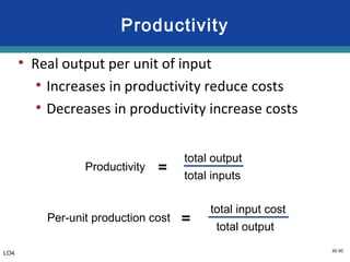
Productivity
• Real outputper unit of input
• Increases in productivity reduce costs
• Decreases in productivity increase costs
Per-unit production cost =
total input cost
total output
Productivity =
total output
total inputs
LO4
31.
30-31
Changes in Short-RunAggregate
Supply
Real domestic output, GDP
Pricelevel
AS1
AS3
AS2
0
• When the input prices
fall or productivity
increases, the short-
run aggregate supply
curve shifts rightward.
• When the input prices
rise or productivity
decreases, the short-
run aggregate supply
curve shifts leftward.
32.
30-32
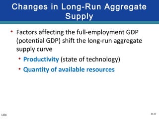
Changes in Long-RunAggregate
Supply
• Factors affecting the full-employment GDP
(potential GDP) shift the long-run aggregate
supply curve
• Productivity (state of technology)
• Quantity of available resources
LO4
33.
30-33
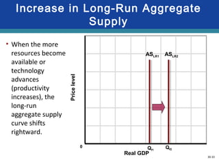
Increase in Long-RunAggregate
Supply
Real GDP
Pricelevel
ASLR1
Qf1
0
ASLR2
Qf2
• When the more
resources become
available or
technology
advances
(productivity
increases), the
long-run
aggregate supply
curve shifts
rightward.
34.
30-34
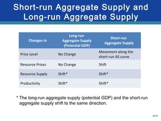
Short-run Aggregate Supplyand
Long-run Aggregate Supply
* The long-run aggregate supply (potential GDP) and the short-run
aggregate supply shift to the same direction.
Changes in
Long-run
Aggregate Supply
(Potential GDP)
Short-run
Aggregate Supply
Price Level No Change
Movement along the
short-run AS curve
Resource Prices No Change Shift
Resource Supply Shift* Shift*
Productivity Shift* Shift*
35.
30-35
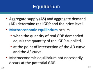
Equilibrium
• Aggregate supply(AS) and aggregate demand
(AD) determine real GDP and the price level.
• Macroeconomic equilibrium occurs
• when the quantity of real GDP demanded
equals the quantity of real GDP supplied.
• at the point of intersection of the AD curve
and the AS curve.
• Macroeconomic equilibrium not necessarily
occurs at the potential GDP.
LO6
36.
30-36
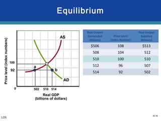
Equilibrium
Real GDP
(billions ofdollars)
Pricelevel(indexnumbers)
100
92
502 510 514
a
b
AD
AS
Real Output
Demanded
(Billions)
Price Level
(Index Number)
Real Output
Supplied
(Billions)
$506 108 $513
508 104 512
510 100 510
512 96 507
514 92 502
0
LO5
37.
30-37
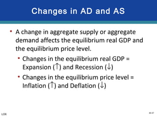
Changes in ADand AS
• A change in aggregate supply or aggregate
demand affects the equilibrium real GDP and
the equilibrium price level.
• Changes in the equilibrium real GDP =
Expansion (↑) and Recession (↓)
• Changes in the equilibrium price level =
Inflation (↑) and Deflation (↓)
LO6
38.
30-38
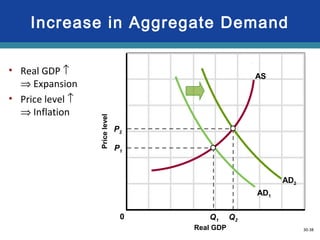
Increase in AggregateDemand
Real GDP
Pricelevel
AD1
AS
P1
P2
Q2Q1
AD2
0
• Real GDP ↑
⇒ Expansion
• Price level ↑
⇒ Inflation
39.
30-39
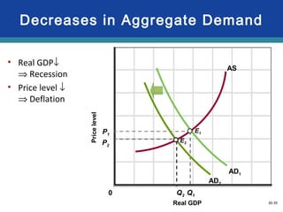
Decreases in AggregateDemand
Real GDP
Pricelevel
AD1
AS
P1
P2
Q2 Q1
AD2
E2
E1
0
• Real GDP↓
⇒ Recession
• Price level ↓
⇒ Deflation
40.
30-40
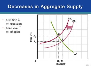
Decreases in AggregateSupply
Real GDP
Pricelevel
AD
AS1
P1
P2
Q2 Q1
AS2
E1
E2
0
• Real GDP ↓
⇒ Recession
• Price level ↑
⇒ Inflation
41.
30-41
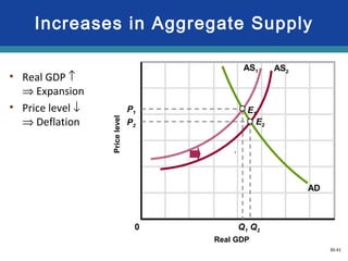
Increases in AggregateSupply
Real GDP
Pricelevel
AS2
P2
Q1
AS1
E1
AD
E2
P1
Q20
• Real GDP ↑
⇒ Expansion
• Price level ↓
⇒ Deflation
42.
30-42
Business Cycle Revisited
•Along the business cycle, we observe
• Expansion with high inflation
• Recession with low inflation or deflation
• These changes can be explained by aggregate
demand fluctuations
• Investment spending fluctuates erratically
• Initiates aggregate expenditure changes
and magnify through multiplier effects
LO6
43.
30-43
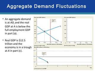
Aggregate Demand Fluctuations
•An aggregate demand
is at AD0 and the real
GDP at A is below the
full-employment GDP
in part (a).
• Real GDP is $12.5
trillion and the
economy is in a trough
at A in part (c).
44.
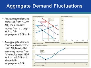
30-44
• An aggregatedemand
increases from AD0 to
AD1, the economy
moves from a trough
at A to full-
employment GDP at B.
• An aggregate demand
continues to increase
from AD1 to AD2, the
economy moves from
full-employment GDP
at B to real GDP at C
above full-
employment GDP.
Aggregate Demand Fluctuations
45.
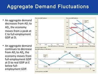
30-45
• An aggregatedemand
decreases from AD2 to
AD3, the economy
moves from a peak at
C to full-employment
GDP at D.
• An aggregate demand
continues to decrease
from AD3 to AD4, the
economy moves from
full-employment GDP
at D to real GDP at E
below full-
employment GDP.
Aggregate Demand Fluctuations
46.
30-46
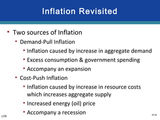
Inflation Revisited
• Twosources of Inflation
• Demand-Pull Inflation
• Inflation caused by increase in aggregate demand
• Excess consumption & government spending
• Accompany an expansion
• Cost-Push Inflation
• Inflation caused by increase in resource costs
which increases aggregate supply
• Increased energy (oil) price
• Accompany a recessionLO6
47.
30-47
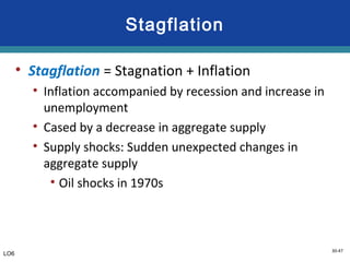
Stagflation
• Stagflation =Stagnation + Inflation
• Inflation accompanied by recession and increase in
unemployment
• Cased by a decrease in aggregate supply
• Supply shocks: Sudden unexpected changes in
aggregate supply
• Oil shocks in 1970s
LO6
30-49
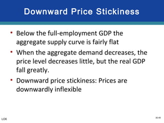
Downward Price Stickiness
•Below the full-employment GDP the
aggregate supply curve is fairly flat
• When the aggregate demand decreases, the
price level decreases little, but the real GDP
fall greatly.
• Downward price stickiness: Prices are
downwardly inflexible
LO6
50.
30-50
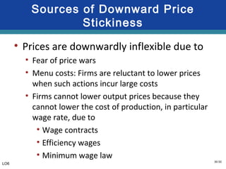
Sources of DownwardPrice
Stickiness
• Prices are downwardly inflexible due to
• Fear of price wars
• Menu costs: Firms are reluctant to lower prices
when such actions incur large costs
• Firms cannot lower output prices because they
cannot lower the cost of production, in particular
wage rate, due to
• Wage contracts
• Efficiency wages
• Minimum wage law
LO6
51.
30-51
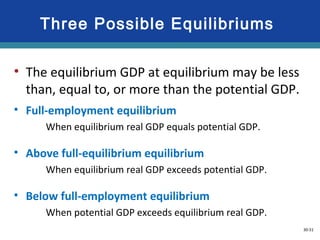
• The equilibriumGDP at equilibrium may be less
than, equal to, or more than the potential GDP.
• Full-employment equilibrium
When equilibrium real GDP equals potential GDP.
• Above full-equilibrium equilibrium
When equilibrium real GDP exceeds potential GDP.
• Below full-employment equilibrium
When potential GDP exceeds equilibrium real GDP.
Three Possible Equilibriums
52.
30-52
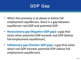
• When theeconomy is at above or below full
employment equilibrium, there is a gap between
equilibrium real GDP and potential GDP.
• Recessionary gap (Negative GDP gap): a gap that
exists when potential GDP exceeds real GDP (below
full-employment equilibrium).
• Inflationary gap (Positive GDP gap): a gap that exists
when real GDP exceeds potential GDP (above full-
employment equilibrium).
GDP Gap
53.
30-53
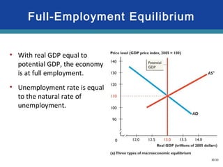
• With realGDP equal to
potential GDP, the economy
is at full employment.
• Unemployment rate is equal
to the natural rate of
unemployment.
Full-Employment Equilibrium
54.
30-54
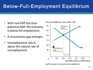
• With realGDP less than
potential GDP, the economy
is below full employment.
• A recessionary gap emerges.
• Unemployment rate is
above the natural rate of
unemployment.
Below-Full-Employment Equilibrium
55.
30-55
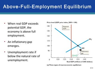
• When realGDP exceeds
potential GDP, the
economy is above full
employment.
• An inflationary gap
emerges.
• Unemployment rate if
below the natural rate of
unemployment.
Above-Full-Employment Equilibrium
56.
30-56
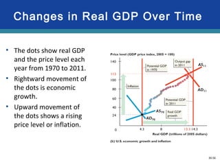
Changes in RealGDP Over Time
• The dots show real GDP
and the price level each
year from 1970 to 2011.
• Rightward movement of
the dots is economic
growth.
• Upward movement of
the dots shows a rising
price level or inflation.
57.
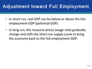
30-57
• In shortrun, real GDP can be below or above the full-
employment GDP (potential GDP).
• In long run, the resource prices (wage rate) gradually
change and shift the short-run supply curve to bring
the economy back to the full employment GDP.
Adjustment toward Full Employment
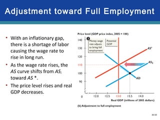
58.
30-58
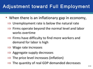
• When thereis an inflationary gap in economy,
⇒ Unemployment rate is below the natural rate
⇒ Firms operate beyond the normal level and labor
works overtime
⇒ Firms have difficulty to find more workers and
demand for labor is high
⇒ Wage rate increases
⇒ Aggregate supply decreases
⇒ The price level increases (inflation)
⇒ The quantity of real GDP demanded decreases
Adjustment toward Full Employment
59.
30-59
• With aninflationary gap,
there is a shortage of labor
causing the wage rate to
rise in long run.
• As the wage rate rises, the
AS curve shifts from AS2
toward AS *.
• The price level rises and real
GDP decreases.
Adjustment toward Full Employment
60.
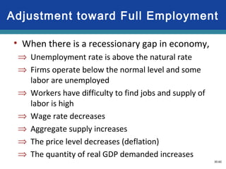
30-60
• When thereis a recessionary gap in economy,
⇒ Unemployment rate is above the natural rate
⇒ Firms operate below the normal level and some
labor are unemployed
⇒ Workers have difficulty to find jobs and supply of
labor is high
⇒ Wage rate decreases
⇒ Aggregate supply increases
⇒ The price level decreases (deflation)
⇒ The quantity of real GDP demanded increases
Adjustment toward Full Employment
61.
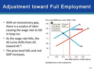
30-61
• With anrecessionary gap,
there is a surplus of labor
causing the wage rate to fall
in long run.
• As the wage rate falls, the
AS curve shifts from AS1
toward AS *.
• The price level falls and real
GDP increases.
Adjustment toward Full Employment
62.
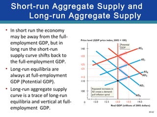
30-62
• In shortrun the economy
may be away from the full-
employment GDP, but in
long run the short-run
supply curve shifts back to
the full-employment GDP.
• Long-run equilibria are
always at full-employment
GDP (Potential GDP).
• Long-run aggregate supply
curve is a trace of long-run
equilibria and vertical at full-
employment GDP.
Short-run Aggregate Supply and
Long-run Aggregate Supply
63.
30-63
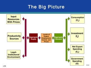
The Big Picture
Levelsof
Output,
Employment,
Income, and
Prices
Aggregate
Demand
Aggregate
Supply
Input
Resources
With Prices
Productivity
Sources
Legal-
Institutional
Environment
Consumption
(Ca)
Investment
(Ig)
Net Export
Spending
(Xn)
Government
Spending
(G)
LO6
Editor's Notes
#2 This chapter introduces the concepts of aggregate demand and aggregate supply, explaining the shapes of the aggregate demand and aggregate supply curves and the forces that cause them to shift. Additionally, the equilibrium levels of prices and real GDP are considered. The chapter analyzes the effects of shifts in the aggregate demand and/or aggregate supply curves on the price level and size of real GDP. This is a “variable price-variable output” model unlike the previous chapter that was an immediate short-run model where prices were assumed fixed. As you will see, this chapter’s model can distinguish between the immediate-short-run, the short-run, and the long-run.
#9 Aggregate demand is a schedule or curve that shows the various amounts of real domestic output that domestic and foreign buyers desire to purchase at each possible price level. The aggregate demand curve shows an inverse relationship between price level and real domestic output.
(The explanation of the inverse relationship is not the same as for demand for a single product, which centered on substitution and income effects. Substitution effect doesn’t apply within the scope of domestically produced goods, since there is no substitute for “everything.” Income effect also doesn’t apply in the aggregate case, since income now varies with aggregate output.)
The explanation of the inverse relationship between price level and real output in aggregate demand are explained by the following three effects.
Real balances effect: When price level falls, the purchasing power of existing financial balances rises, which can increase spending.
Interest rate effect: A decline in price level means lower interest rates that can increase levels of certain types of spending.
Foreign purchases effect: When price level falls, other things being equal, U.S. prices will fall relative to foreign prices, which will tend to increase spending on U.S. exports and also decrease import spending in favor of U.S. products that compete with imports (similar to the substitution effect).
#10 This figure depicts the aggregate demand curve. The downsloping aggregate demand curve, AD, indicates an inverse (or negative) relationship between the price level and the amount of real output purchased.
#11 Aggregate demand is a schedule or curve that shows the various amounts of real domestic output that domestic and foreign buyers desire to purchase at each possible price level. The aggregate demand curve shows an inverse relationship between price level and real domestic output.
(The explanation of the inverse relationship is not the same as for demand for a single product, which centered on substitution and income effects. Substitution effect doesn’t apply within the scope of domestically produced goods, since there is no substitute for “everything.” Income effect also doesn’t apply in the aggregate case, since income now varies with aggregate output.)
The explanation of the inverse relationship between price level and real output in aggregate demand are explained by the following three effects.
Real balances effect: When price level falls, the purchasing power of existing financial balances rises, which can increase spending.
Interest rate effect: A decline in price level means lower interest rates that can increase levels of certain types of spending.
Foreign purchases effect: When price level falls, other things being equal, U.S. prices will fall relative to foreign prices, which will tend to increase spending on U.S. exports and also decrease import spending in favor of U.S. products that compete with imports (similar to the substitution effect).
#12 Aggregate demand is a schedule or curve that shows the various amounts of real domestic output that domestic and foreign buyers desire to purchase at each possible price level. The aggregate demand curve shows an inverse relationship between price level and real domestic output.
(The explanation of the inverse relationship is not the same as for demand for a single product, which centered on substitution and income effects. Substitution effect doesn’t apply within the scope of domestically produced goods, since there is no substitute for “everything.” Income effect also doesn’t apply in the aggregate case, since income now varies with aggregate output.)
The explanation of the inverse relationship between price level and real output in aggregate demand are explained by the following three effects.
Real balances effect: When price level falls, the purchasing power of existing financial balances rises, which can increase spending.
Interest rate effect: A decline in price level means lower interest rates that can increase levels of certain types of spending.
Foreign purchases effect: When price level falls, other things being equal, U.S. prices will fall relative to foreign prices, which will tend to increase spending on U.S. exports and also decrease import spending in favor of U.S. products that compete with imports (similar to the substitution effect).
#13 Aggregate demand is a schedule or curve that shows the various amounts of real domestic output that domestic and foreign buyers desire to purchase at each possible price level. The aggregate demand curve shows an inverse relationship between price level and real domestic output.
(The explanation of the inverse relationship is not the same as for demand for a single product, which centered on substitution and income effects. Substitution effect doesn’t apply within the scope of domestically produced goods, since there is no substitute for “everything.” Income effect also doesn’t apply in the aggregate case, since income now varies with aggregate output.)
The explanation of the inverse relationship between price level and real output in aggregate demand are explained by the following three effects.
Real balances effect: When price level falls, the purchasing power of existing financial balances rises, which can increase spending.
Interest rate effect: A decline in price level means lower interest rates that can increase levels of certain types of spending.
Foreign purchases effect: When price level falls, other things being equal, U.S. prices will fall relative to foreign prices, which will tend to increase spending on U.S. exports and also decrease import spending in favor of U.S. products that compete with imports (similar to the substitution effect).
#14 Determinants of aggregate demand are the “other things” (besides price level) that can cause a shift or change in demand.
Effects of the following determinants are discussed in more detail on the slides following the graph.
1. Changes in consumer spending, which can be caused by changes in several factors: consumer wealth, consumer expectations, household debt, and taxes.
2. Changes in investment spending, which can be caused by changes in several factors: interest rates. Another factor is expected returns which are a function of: expected future business conditions, technology, degree of excess capacity, and business taxes.
Changes in government spending
Changes in net export spending unrelated to price level, which may be caused by changes in other factors such as: national incomes abroad and exchange rates.
#15 This figure shows changes in aggregate demand.
A change in one or more of the listed determinants of aggregate demand will shift the aggregate demand curve. The rightward shift from AD1 to AD2 represents an increase in aggregate demand; the leftward shift from AD1 to AD3 shows a decrease in aggregate demand. The vertical distances between AD1 and the dashed lines represent the initial changes in spending. Through the multiplier effect, that spending produces the full shifts of the curves.
#16 Consumer wealth is the difference between household assets (homes and stocks and bonds) and liabilities (loans and credit cards). The value of the assets can change and the consumer will react by spending more as asset values increase and spending less as asset values decrease.
Households can borrow in order to spend more which increases AD and if the household reduces spending in order to pay off household debt, AD decreases.
Expectations of future higher incomes or higher prices will increase current household spending and AD; expectations of lower household spending or lower prices will decrease AD.
A reduction in personal income taxes increases disposable income and increases spending by the household, increasing AD; an increase in taxes will decrease disposable income and decrease household spending, decreasing AD.
#17 Investment spending is spending on capital goods. Increases in investment spending increases AD; decreases in investment goods decreases AD.
As real interest rates increase, the cost of borrowing increases and subsequently less will be borrowed resulting in less money spent, reducing AD. On the other hand, a decrease in real interest rates will increase borrowing and subsequently investment spending will increase AD.
If business owners and managers are optimistic about future expected returns they will spend more now increasing AD and if expected returns are less than favorable they will spend less now reducing AD.
New technologies enhance future expected returns and thus motivate businesses to spend money on the new technology increasing AD.
If excess capacity increases, businesses will decrease current spending, decreasing AD. If excess capacity decreases, businesses will increase spending in order to expand operations, increasing AD.
An increase in business taxes will decrease the amount of after-tax income for businesses, reducing the amount of spending businesses are capable of, reducing AD. A decrease in business taxes will have the opposite effect on AD.
#18 Other things equal, if government spending increases, AD increases. An example of government spending is more, or less, transportation projects.
If government spending decreases, AD decreases. An example of this is more, or less, military spending.
#19 If net export spending rises, AD rises. If net export spending declines, AD declines. As the national incomes of trading partners of the U.S. increase, they are more able to purchase U.S. produced goods and services which increases AD. If the foreign nations’ incomes decline, the opposite occurs.
If the dollar depreciates relative to another country’s currency, AD increases. Depreciation of the dollar encourages U.S. exports since U.S. products become less expensive, as foreign buyers can obtain more dollars for their currency. Conversely, dollar depreciation discourages import buying in the U.S. because our dollars can’t be exchanged for as much foreign currency.
AD can decrease through changes in currency exchange rates if the U.S. dollar appreciates relative to another country’s currency. The currency appreciation of the dollar discourages U.S. exports because now U.S. goods are relatively more expensive than before since it takes more of the foreign currency to buy the U.S. dollar. This will also encourage more import spending since the U.S. dollar can buy more of another nation’s currency than before. Net exports will decline which reduces AD.
#20 Aggregate supply is a schedule or curve showing the level of real domestic output available at each possible price level. The relationship is determined on the basis of whether input prices and output prices are fixed or flexible.
In the immediate short run, both input prices and output prices are fixed. The input prices are fixed by contractual agreements such as labor contracts. Output prices may be fixed as a result of issuance of catalogs or price lists that are in effect for a stated period of time.
In the short run, input prices are fixed but output prices are variable.
In the long run, input prices and output prices can vary.
#21 Aggregate supply is a schedule or curve showing the level of real domestic output available at each possible price level. The relationship is determined on the basis of whether input prices and output prices are fixed or flexible.
In the immediate short run, both input prices and output prices are fixed. The input prices are fixed by contractual agreements such as labor contracts. Output prices may be fixed as a result of issuance of catalogs or price lists that are in effect for a stated period of time.
In the short run, input prices are fixed but output prices are variable.
In the long run, input prices and output prices can vary.
#22 Aggregate supply is a schedule or curve showing the level of real domestic output available at each possible price level. The relationship is determined on the basis of whether input prices and output prices are fixed or flexible.
In the immediate short run, both input prices and output prices are fixed. The input prices are fixed by contractual agreements such as labor contracts. Output prices may be fixed as a result of issuance of catalogs or price lists that are in effect for a stated period of time.
In the short run, input prices are fixed but output prices are variable.
In the long run, input prices and output prices can vary.
#23 Aggregate supply is a schedule or curve showing the level of real domestic output available at each possible price level. The relationship is determined on the basis of whether input prices and output prices are fixed or flexible.
In the immediate short run, both input prices and output prices are fixed. The input prices are fixed by contractual agreements such as labor contracts. Output prices may be fixed as a result of issuance of catalogs or price lists that are in effect for a stated period of time.
In the short run, input prices are fixed but output prices are variable.
In the long run, input prices and output prices can vary.
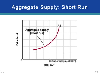
#24 The figure shows the aggregate supply curve in the short run.
The upsloping aggregate supply curve AS indicates a direct (or positive) relationship between the price level and the amount of real output that firms will offer for sale. The AS curve is relatively flat below the full-employment output because unemployed resources and unused capacity allow firms to respond to price-level rises with large increases in real output. It is relatively steep beyond the full-employment output because resource shortages and capacity limitations make it difficult to expand real output as the price level rises.
AS slopes upward because with input prices fixed, rising prices increase real profits and declining prices result in decreases in real profits.
#25 This figure reflects aggregate supply in the long run. The long-run aggregate supply curve, ASLR, is vertical at the full-employment level of real GDP (Qf) because in the long run wages and other input prices rise and fall to match changes in the price level. So price-level changes do not affect firms’ profits and thus they create no incentive for firms to alter their output. In the long run, the economy will produce the full-employment output level no matter what the price level is because profits always adjust to give firms exactly the right profit incentive to produce exactly the full employment output level.
#26 Determinants of aggregate supply are the “other things” besides price level that cause changes or shifts in aggregate supply at each price level.
Changes that reduce per-unit production costs shift the aggregate supply curve to the right; changes that increase per-unit production costs shift AS left.
(References to “aggregate supply” in the remainder of the chapter apply to the short run curve unless otherwise noted.)
#27 Determinants of aggregate supply are the “other things” besides price level that cause changes or shifts in aggregate supply at each price level.
Changes that reduce per-unit production costs shift the aggregate supply curve to the right; changes that increase per-unit production costs shift AS left.
(References to “aggregate supply” in the remainder of the chapter apply to the short run curve unless otherwise noted.)
#28 Determinants of aggregate supply are the “other things” besides price level that cause changes or shifts in aggregate supply at each price level.
Changes that reduce per-unit production costs shift the aggregate supply curve to the right; changes that increase per-unit production costs shift AS left.
(References to “aggregate supply” in the remainder of the chapter apply to the short run curve unless otherwise noted.)
#29 Determinants of aggregate supply are the “other things” besides price level that cause changes or shifts in aggregate supply at each price level.
Changes that reduce per-unit production costs shift the aggregate supply curve to the right; changes that increase per-unit production costs shift AS left.
(References to “aggregate supply” in the remainder of the chapter apply to the short run curve unless otherwise noted.)
#30 Determinants of aggregate supply are the “other things” besides price level that cause changes or shifts in aggregate supply at each price level.
Changes that reduce per-unit production costs shift the aggregate supply curve to the right; changes that increase per-unit production costs shift AS left.
(References to “aggregate supply” in the remainder of the chapter apply to the short run curve unless otherwise noted.)
#31 Changes in productivity (productivity = real output divided by input) can cause changes in per-unit production cost (production cost per unit = total input cost divided by units of output). If productivity rises, unit production costs will fall. This can shift aggregate supply to the right and lower prices. The reverse is true when productivity falls. Productivity improvement is very important in business efforts to reduce costs.
#32 This figure illustrates changes in aggregate supply. A change in one or more of the AS determinants listed on the next slide will shift the aggregate supply curve. The rightward shift of the aggregate supply curve from AS1 to AS2 represents an increase in aggregate supply; the leftward shift of the curve from AS1 to AS3 shows a decrease in aggregate supply.
#33 Determinants of aggregate supply are the “other things” besides price level that cause changes or shifts in aggregate supply at each price level.
Changes that reduce per-unit production costs shift the aggregate supply curve to the right; changes that increase per-unit production costs shift AS left.
(References to “aggregate supply” in the remainder of the chapter apply to the short run curve unless otherwise noted.)
#34 This figure reflects aggregate supply in the long run. The long-run aggregate supply curve, ASLR, is vertical at the full-employment level of real GDP (Qf) because in the long run wages and other input prices rise and fall to match changes in the price level. So price-level changes do not affect firms’ profits and thus they create no incentive for firms to alter their output. In the long run, the economy will produce the full-employment output level no matter what the price level is because profits always adjust to give firms exactly the right profit incentive to produce exactly the full employment output level.
#36 If AD decreases, recession and cyclical unemployment may result. Prices don’t fall easily.
Fear of price wars keeps prices from being reduced. Businesses fear that if they decrease their price, their rivals may decrease their price even more which could result in a “price war”: successively deeper and deeper price cuts which result in reduced profits for all of the firms.
Menu costs discourage repeated price changes. Menu costs are the costs businesses incur from printing new price lists or catalogs, re-pricing inventory, and communicating new prices to customers. Firms may wait and see if the decline in aggregate demand is permanent.
Large parts of the work force are under wage contracts that are not flexible, therefore businesses can’t afford to reduce the price of their products.
Employers are reluctant to cut wages because of the impact on employee morale, effort, and productivity. Employers seek to pay efficiency wages – wages that maximize work effort and productivity, minimizing cost.
The minimum wage law is a legal minimum wage for low-skilled labor. Firms that pay minimum wages cannot reduce them when aggregate demand declines.
#37 This figure shows the equilibrium price level and equilibrium real GDP. The intersection of the aggregate demand curve and the aggregate supply curve determines the economy’s equilibrium price level. At the equilibrium price level of 100 (in index-value terms), the $510 billion of real output demanded matches the $510 billion of real output supplied. So the equilibrium GDP is $510 billion.
#38 If AD decreases, recession and cyclical unemployment may result. Prices don’t fall easily.
Fear of price wars keeps prices from being reduced. Businesses fear that if they decrease their price, their rivals may decrease their price even more which could result in a “price war”: successively deeper and deeper price cuts which result in reduced profits for all of the firms.
Menu costs discourage repeated price changes. Menu costs are the costs businesses incur from printing new price lists or catalogs, re-pricing inventory, and communicating new prices to customers. Firms may wait and see if the decline in aggregate demand is permanent.
Large parts of the work force are under wage contracts that are not flexible, therefore businesses can’t afford to reduce the price of their products.
Employers are reluctant to cut wages because of the impact on employee morale, effort, and productivity. Employers seek to pay efficiency wages – wages that maximize work effort and productivity, minimizing cost.
The minimum wage law is a legal minimum wage for low-skilled labor. Firms that pay minimum wages cannot reduce them when aggregate demand declines.
#39 This figure shows an increase in aggregate demand that causes demand-pull inflation. The increase in aggregate demand from AD1 to AD2 causes demand-pull inflation, shown as the rise in the price level from P1 to P2. It also causes an inflationary GDP gap of Q1 minus Qf. The rise in the price level reduces the size of the multiplier effect. If the price level had remained at P1, the increase in aggregate demand from AD1 to AD2 would increase output from Qf to Q2 and the multiplier would have been at full strength. But because of the increase in the price level, real output increases only from Qf to Q1 and the multiplier effect is reduced.
#40 This figure shows a decrease in aggregate demand that causes a recession. If the price level is downwardly inflexible at P1, a decline of aggregate demand from AD1 to AD2 will move the economy leftward from a to b along the horizontal broken-line segment and reduce real GDP from Qf to Q1. Idle production capacity, cyclical unemployment, and a recessionary GDP gap (of Q1 minus Qf) will result. If the price level were flexible downward, the decline in aggregate demand would move the economy depicted from a to c instead of from a to b.
#41 This figure reflects a decrease in aggregate supply that causes cost-push inflation. A leftward shift of aggregate supply from AS1 to AS2 raises the price level from P1 to P2 and produces cost-push inflation. Real output declines and a recessionary GDP gap (of Q1 minus Qf) occurs.
#42 This figure illustrates growth, full employment, and relative price stability. Normally, an increase in aggregate demand from AD1 to AD2 would move the economy from a to b along AS1. Real output would expand to Q2, and inflation would result (P1 to P3). But in the late 1990s, significant increases in productivity shifted the aggregate supply curve, as shown by AS1 to AS2. The economy moved from a to c rather than from a to b. It experienced strong economic growth (Q1 to Q3), full employment, and only very mild inflation (P1 to P2) before receding in March 2001.
#43 If AD decreases, recession and cyclical unemployment may result. Prices don’t fall easily.
Fear of price wars keeps prices from being reduced. Businesses fear that if they decrease their price, their rivals may decrease their price even more which could result in a “price war”: successively deeper and deeper price cuts which result in reduced profits for all of the firms.
Menu costs discourage repeated price changes. Menu costs are the costs businesses incur from printing new price lists or catalogs, re-pricing inventory, and communicating new prices to customers. Firms may wait and see if the decline in aggregate demand is permanent.
Large parts of the work force are under wage contracts that are not flexible, therefore businesses can’t afford to reduce the price of their products.
Employers are reluctant to cut wages because of the impact on employee morale, effort, and productivity. Employers seek to pay efficiency wages – wages that maximize work effort and productivity, minimizing cost.
The minimum wage law is a legal minimum wage for low-skilled labor. Firms that pay minimum wages cannot reduce them when aggregate demand declines.
#47 If AD decreases, recession and cyclical unemployment may result. Prices don’t fall easily.
Fear of price wars keeps prices from being reduced. Businesses fear that if they decrease their price, their rivals may decrease their price even more which could result in a “price war”: successively deeper and deeper price cuts which result in reduced profits for all of the firms.
Menu costs discourage repeated price changes. Menu costs are the costs businesses incur from printing new price lists or catalogs, re-pricing inventory, and communicating new prices to customers. Firms may wait and see if the decline in aggregate demand is permanent.
Large parts of the work force are under wage contracts that are not flexible, therefore businesses can’t afford to reduce the price of their products.
Employers are reluctant to cut wages because of the impact on employee morale, effort, and productivity. Employers seek to pay efficiency wages – wages that maximize work effort and productivity, minimizing cost.
The minimum wage law is a legal minimum wage for low-skilled labor. Firms that pay minimum wages cannot reduce them when aggregate demand declines.
#48 If AD decreases, recession and cyclical unemployment may result. Prices don’t fall easily.
Fear of price wars keeps prices from being reduced. Businesses fear that if they decrease their price, their rivals may decrease their price even more which could result in a “price war”: successively deeper and deeper price cuts which result in reduced profits for all of the firms.
Menu costs discourage repeated price changes. Menu costs are the costs businesses incur from printing new price lists or catalogs, re-pricing inventory, and communicating new prices to customers. Firms may wait and see if the decline in aggregate demand is permanent.
Large parts of the work force are under wage contracts that are not flexible, therefore businesses can’t afford to reduce the price of their products.
Employers are reluctant to cut wages because of the impact on employee morale, effort, and productivity. Employers seek to pay efficiency wages – wages that maximize work effort and productivity, minimizing cost.
The minimum wage law is a legal minimum wage for low-skilled labor. Firms that pay minimum wages cannot reduce them when aggregate demand declines.
#50 If AD decreases, recession and cyclical unemployment may result. Prices don’t fall easily.
Fear of price wars keeps prices from being reduced. Businesses fear that if they decrease their price, their rivals may decrease their price even more which could result in a “price war”: successively deeper and deeper price cuts which result in reduced profits for all of the firms.
Menu costs discourage repeated price changes. Menu costs are the costs businesses incur from printing new price lists or catalogs, re-pricing inventory, and communicating new prices to customers. Firms may wait and see if the decline in aggregate demand is permanent.
Large parts of the work force are under wage contracts that are not flexible, therefore businesses can’t afford to reduce the price of their products.
Employers are reluctant to cut wages because of the impact on employee morale, effort, and productivity. Employers seek to pay efficiency wages – wages that maximize work effort and productivity, minimizing cost.
The minimum wage law is a legal minimum wage for low-skilled labor. Firms that pay minimum wages cannot reduce them when aggregate demand declines.
#51 If AD decreases, recession and cyclical unemployment may result. Prices don’t fall easily.
Fear of price wars keeps prices from being reduced. Businesses fear that if they decrease their price, their rivals may decrease their price even more which could result in a “price war”: successively deeper and deeper price cuts which result in reduced profits for all of the firms.
Menu costs discourage repeated price changes. Menu costs are the costs businesses incur from printing new price lists or catalogs, re-pricing inventory, and communicating new prices to customers. Firms may wait and see if the decline in aggregate demand is permanent.
Large parts of the work force are under wage contracts that are not flexible, therefore businesses can’t afford to reduce the price of their products.
Employers are reluctant to cut wages because of the impact on employee morale, effort, and productivity. Employers seek to pay efficiency wages – wages that maximize work effort and productivity, minimizing cost.
The minimum wage law is a legal minimum wage for low-skilled labor. Firms that pay minimum wages cannot reduce them when aggregate demand declines.
#58 Don’t neglect the predictions of the model. This is the payoff for the student. With this simple model, we can now say quite a lot about growth, inflation, and the business cycle. However, when you do so, be aware that the AS-AD model predicts a fall in the price level when either aggregate demand decreases or aggregate supply increases. And the model predicts that real GDP decreases when either aggregate supply or aggregate demand decreases. But, some students object by pointing out that GDP rarely decreases and the price level rarely falls. These students are bothered by this apparent mismatch between the predictions of the model and the observed economy. The best way to handle this issue is to emphasize that in our actual economy, aggregate supply and aggregate demand almost always are increasing. When we use the model to simulate the effects of a decrease in either aggregate supply and aggregate demand, we’re studying what happens relative to the trends in real GDP and the price level. A fall in the price level in the model translates into a lower price level than would otherwise have occurred and a slowing of inflation. The story is similar for real GDP.
#59 Don’t neglect the predictions of the model. This is the payoff for the student. With this simple model, we can now say quite a lot about growth, inflation, and the business cycle. However, when you do so, be aware that the AS-AD model predicts a fall in the price level when either aggregate demand decreases or aggregate supply increases. And the model predicts that real GDP decreases when either aggregate supply or aggregate demand decreases. But, some students object by pointing out that GDP rarely decreases and the price level rarely falls. These students are bothered by this apparent mismatch between the predictions of the model and the observed economy. The best way to handle this issue is to emphasize that in our actual economy, aggregate supply and aggregate demand almost always are increasing. When we use the model to simulate the effects of a decrease in either aggregate supply and aggregate demand, we’re studying what happens relative to the trends in real GDP and the price level. A fall in the price level in the model translates into a lower price level than would otherwise have occurred and a slowing of inflation. The story is similar for real GDP.
#61 Don’t neglect the predictions of the model. This is the payoff for the student. With this simple model, we can now say quite a lot about growth, inflation, and the business cycle. However, when you do so, be aware that the AS-AD model predicts a fall in the price level when either aggregate demand decreases or aggregate supply increases. And the model predicts that real GDP decreases when either aggregate supply or aggregate demand decreases. But, some students object by pointing out that GDP rarely decreases and the price level rarely falls. These students are bothered by this apparent mismatch between the predictions of the model and the observed economy. The best way to handle this issue is to emphasize that in our actual economy, aggregate supply and aggregate demand almost always are increasing. When we use the model to simulate the effects of a decrease in either aggregate supply and aggregate demand, we’re studying what happens relative to the trends in real GDP and the price level. A fall in the price level in the model translates into a lower price level than would otherwise have occurred and a slowing of inflation. The story is similar for real GDP.
#64 This figure illustrates the many concepts and principles discussed in the preceding chapters and how they relate to one another.