This document covers basic macroeconomic relationships including:
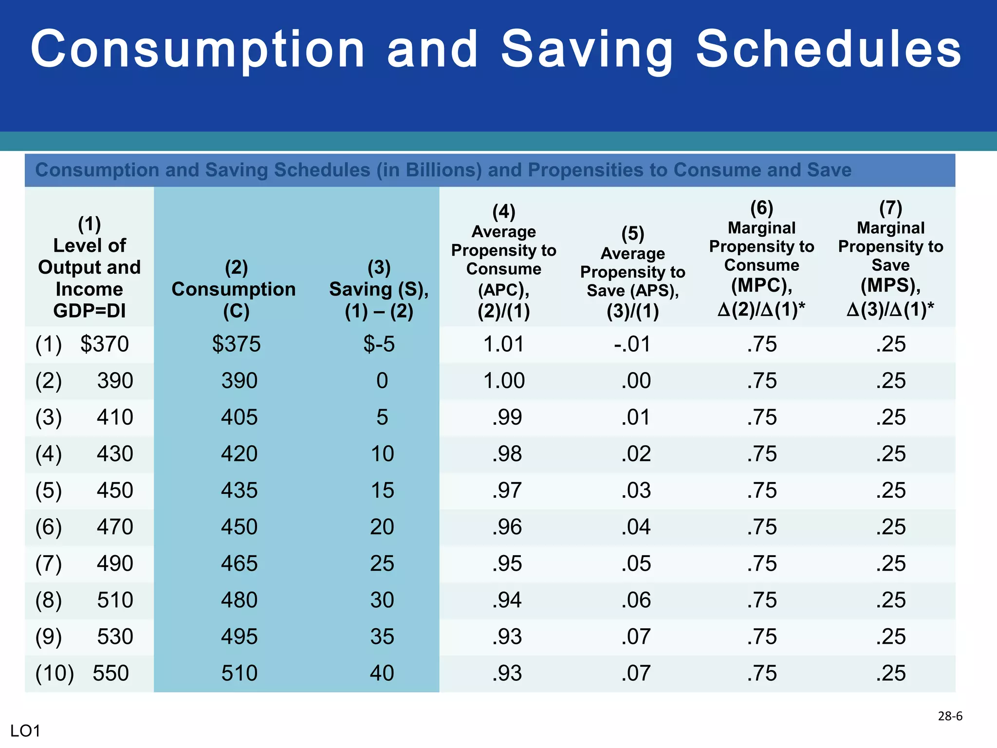
1) How consumption and saving are primarily determined by disposable income, with consumption directly related to and saving inversely related to income levels.
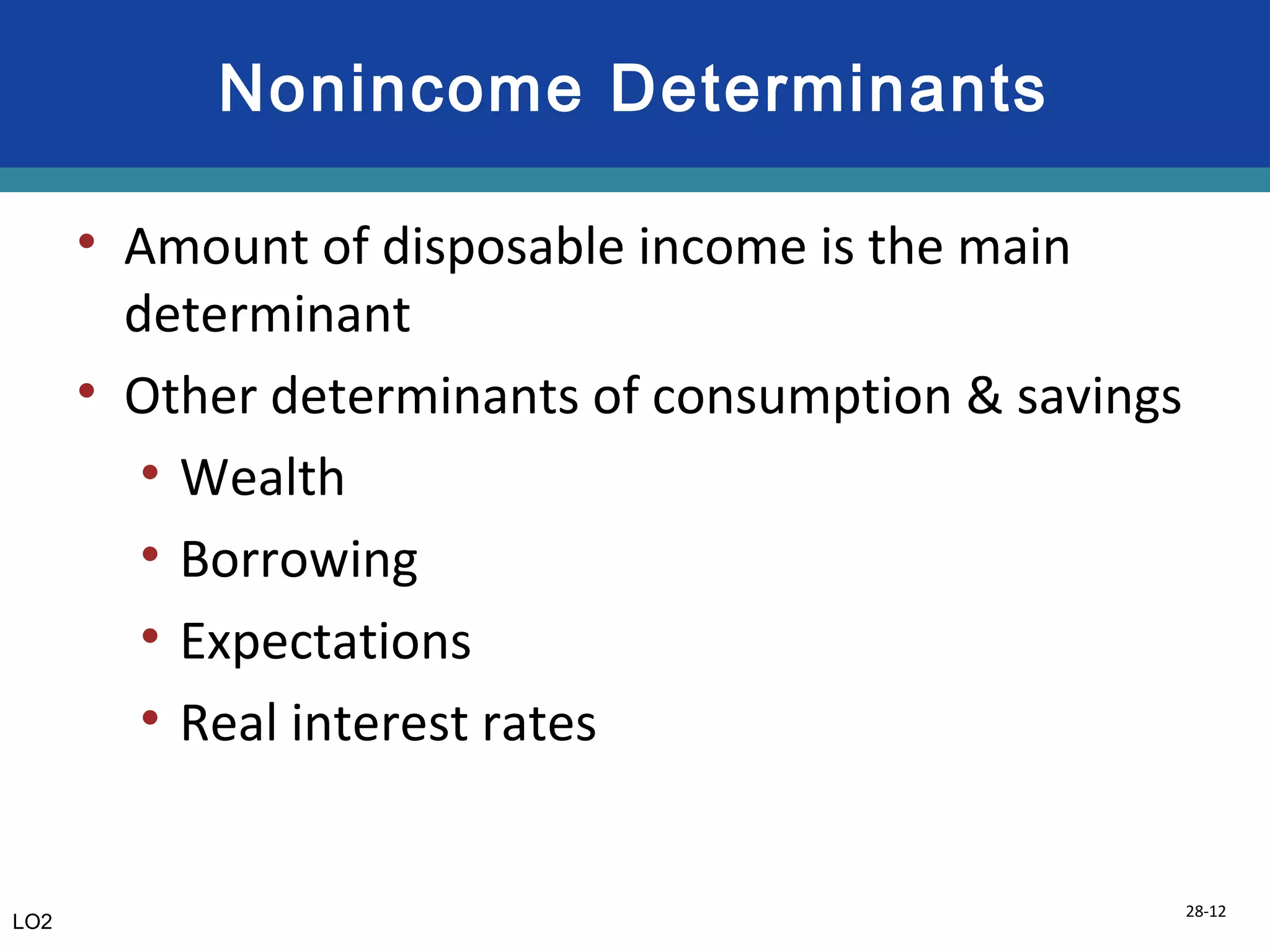
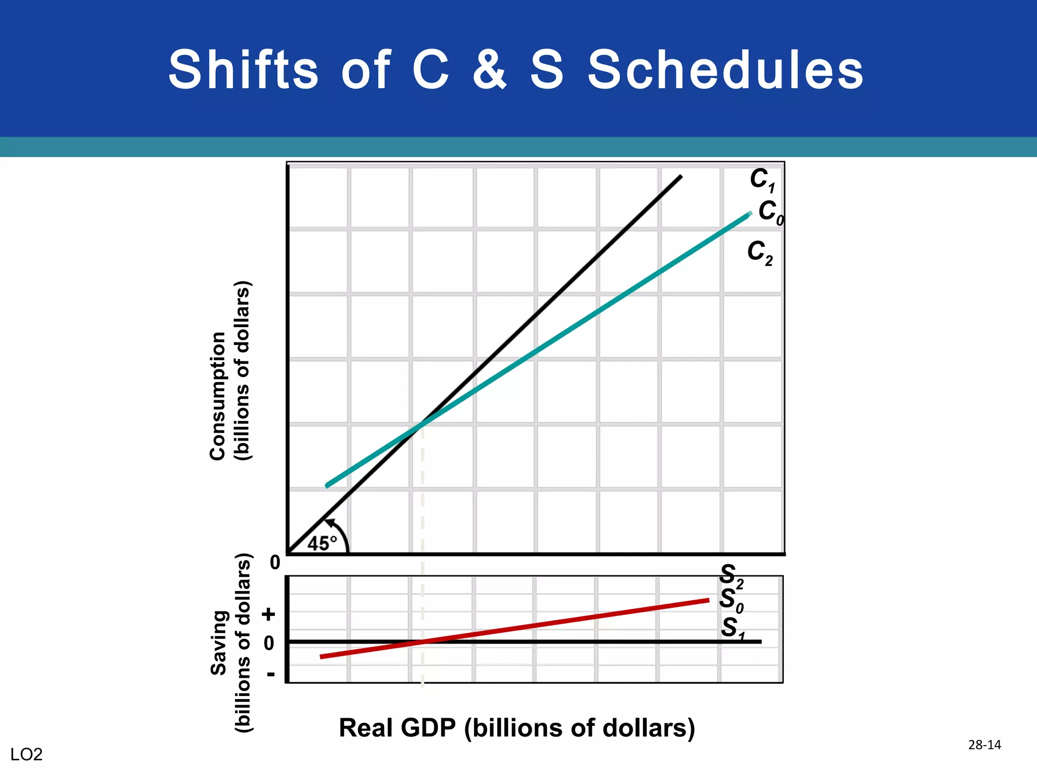
2) Other factors besides income that can affect consumption and saving such as wealth, borrowing, expectations, and interest rates.
3) How investment is directly related to real interest rates, with lower rates stimulating more investment, and various other non-interest factors that can affect investment levels.
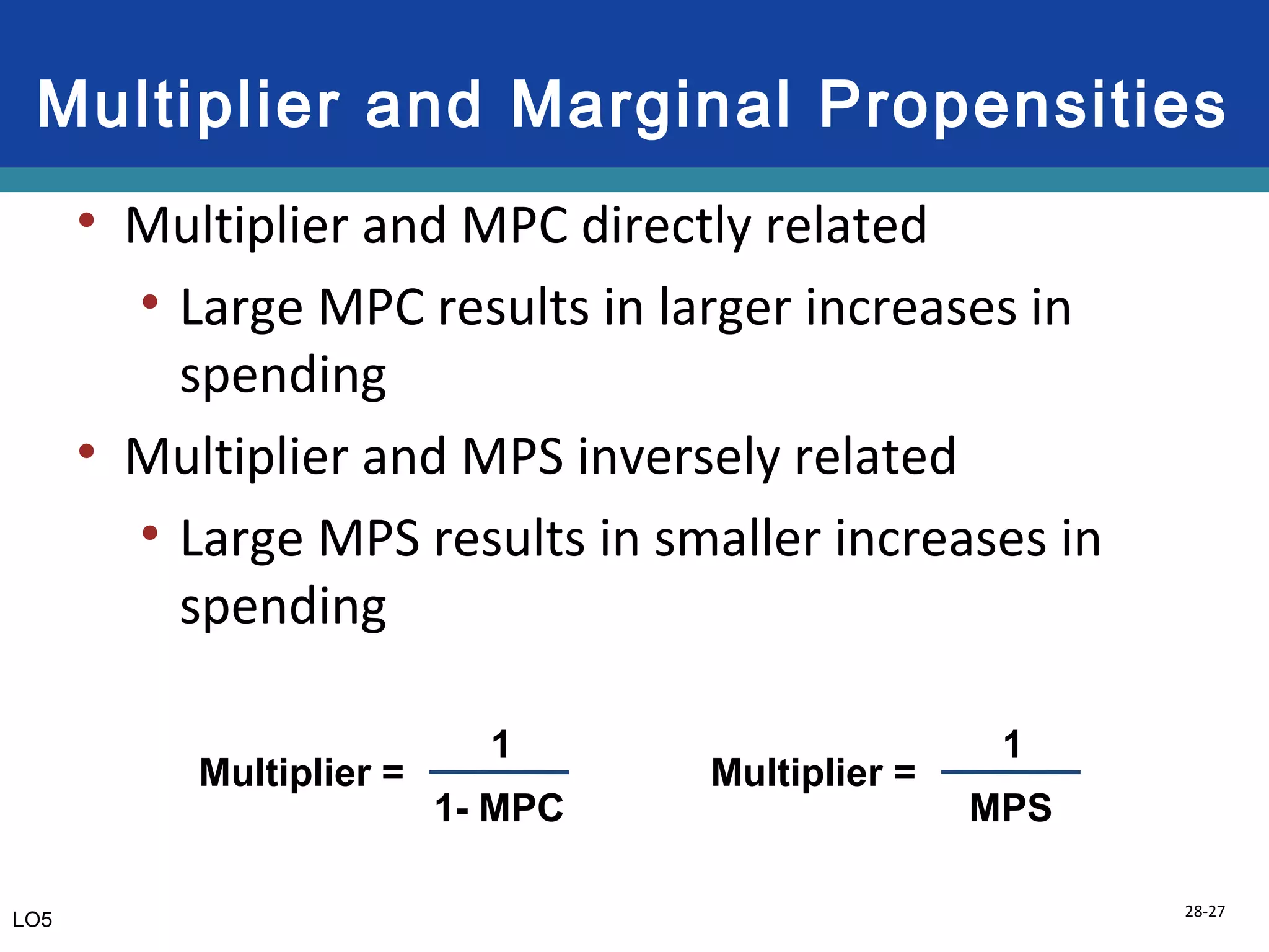
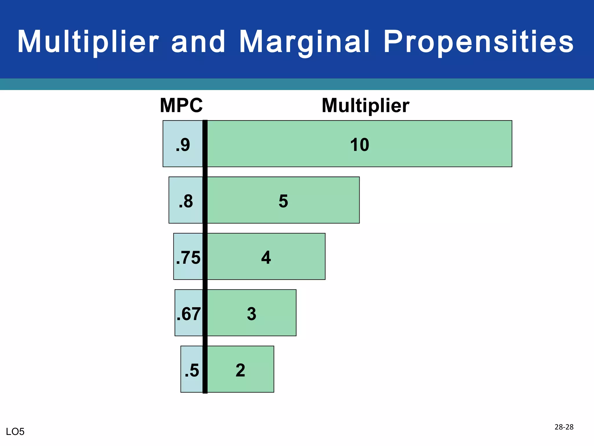
4) How changes in investment or other spending components can multiply, with the multiplier effect magnifying the initial change in spending into a larger change in real GDP.
This document discusses national income accounting and gross domestic product (GDP) as measures of an economy's overall performance. It explains that the Bureau of Economic Analysis compiles National Income and Product Accounts to assess the health of the economy, track its long-run trends, and help formulate policy. GDP is defined as the monetary value of all final goods and services produced within a country in a given period of time. The two main approaches to calculating GDP are the expenditures approach and the income approach.
Economic growth can be measured as an increase in real GDP or real GDP per capita over time. Real GDP in the US has increased over sixfold since 1950, growing at an average annual rate of 3.1%. Real GDP per capita has increased over threefold, growing at around 2% per year. Factors that determine economic growth include increases in the quantity and quality of labor, capital, technology, and efficiency. Productivity growth, driven by technological advances, education, and capital investment, has been a major contributor to economic growth. While some argue that sustained growth may not be environmentally sustainable, most economists view economic growth as increasing living standards and enabling solutions to problems through human innovation.
LO1. Explain how sticky prices relate to the AE model.
LO2. Explain how an economy’s investment schedule is derived from the investment demand curve & an interest rate.
LO3. The table shows different levels of output and the corresponding levels of consumption, investment, exports and aggregate expenditures to determine the equilibrium level of output where aggregate expenditures equals output.
LO4. Equilibrium is also characterized by savings equaling investment and consumption being less than output due to savings being a leakage from the circular flow of spending.
This document discusses business cycles, unemployment, and inflation. It begins by describing the four phases of the business cycle: peak, recession, trough, and expansion. It then discusses different types of unemployment like frictional, structural, and cyclical unemployment. Finally, it explains the two types of inflation - demand-pull inflation caused by excess spending, and cost-push inflation caused by increases in input costs. It also discusses how inflation can redistribute incomes and outlines some of the economic costs of unemployment like reduced GDP and higher social costs.
The document provides information about an economics class, including:
1) It welcomes students back and congratulates those with good grades from the previous semester.
2) It outlines the course details - the name, venue, tutor, and lecturer.
3) It explains the aims of the class include understanding macroeconomics and achieving an A grade.
This document discusses basic macroeconomic relationships including consumption, investment, and the multiplier effect. It contains the following key points:
1) Consumption is directly related to disposable income, with a marginal propensity to consume (MPC) of typically around 0.75. This means that an additional $1 of income leads to $0.75 of additional consumption.
2) Investment demand is negatively related to real interest rates, with the investment demand curve sloping downward. Factors like expectations, costs, and technological change can cause shifts in the investment demand curve.
3) The multiplier effect describes how an initial change in spending, such as an increase in investment, leads to a multiplied impact on overall
This document discusses key aspects of fiscal policy and the federal budget in the United States. It begins by defining the federal budget and its two main purposes of financing government activities and achieving macroeconomic goals. It then explains how fiscal policy uses changes in government spending and taxes to influence aggregate demand and achieve full employment, inflation control, and economic growth. The document also discusses the effects of expansionary and contractionary fiscal policy, discretionary versus built-in (automatic) fiscal policy, and how to evaluate the stance of fiscal policy using cyclically adjusted budget deficits and surpluses.
The document discusses key macroeconomic concepts including aggregate demand, aggregate supply, the consumption function, investment function, and the multiplier. It provides details on how each of these factors impact macroeconomic variables like output, employment, prices, and trade. It also examines the relationship between aggregate demand and supply using the AD-AS framework and how this intersection determines macroeconomic equilibrium.
Introduction to Macroeconomics: National IncomeUpananda Witta
This document provides an overview of macroeconomics concepts across several chapters. It defines macroeconomics as dealing with aggregate economic metrics rather than individual parts. Key concepts discussed include the circular flow of income and goods between households, firms, and the government. The document also examines gross domestic product, national income, consumption, investment, fiscal and monetary policy, and how international trade impacts a country's national income. Multiple diagrams and equations are presented to illustrate macroeconomic relationships between sectors.
This document provides an overview of aggregate demand, including its basic concept, determinants, components, and relationship to aggregate supply. It defines aggregate demand as the total quantity of goods and services demanded in an economy at a given price level. The four main components that make up aggregate demand are consumption, investment, government spending, and net exports. Each component is affected by various economic factors, such as consumer confidence, interest rates, fiscal policy, and exchange rates. The document also discusses how aggregate demand curves can be used to model the aggregate demand-aggregate supply relationship in an economy.
This document defines and explains aggregate demand. It notes that aggregate demand is the total demand for finished goods and services in an economy, consisting of consumer goods, capital goods, exports, imports, and government spending. It was introduced by economist John Maynard Keynes and focuses on using fiscal and monetary policy to address economic recessions. The document then provides details on Keynesian economics, the Great Depression that prompted Keynes' work, and how to calculate aggregate demand using the equation of consumption, investment, government spending, and net exports. It also discusses factors that can cause the aggregate demand curve to shift in or out.
The document summarizes key concepts from Chapter 31 of an economics textbook on the aggregate expenditures model. It introduces the model's assumptions, components of aggregate expenditures (C + I + G + NX), and how equilibrium GDP is achieved when aggregate expenditures equal real GDP. It explains how changes in investment, net exports, government purchases affect the aggregate expenditures schedule and equilibrium GDP. The multiplier effect of changes in investment on equilibrium GDP is also discussed.
The document discusses key macroeconomic concepts including aggregate demand, aggregate supply, the consumption function, investment function, and the multiplier. It provides the following key points:
- Aggregate demand is the total demand for final goods and services in an economy. It is affected by factors like money, taxes, prices, and trade.
- Aggregate supply represents the maximum output an economy can produce at full employment. It can shift due to changes in inputs like labor, capital, technology and costs.
- The consumption function explains autonomous and induced consumption and how consumption relates to disposable income based on the marginal propensity to consume.
- The investment function depends on interest rates, profit expectations and taxes, and
The document discusses key economic goals and indicators used to measure economic performance, including low inflation, low unemployment, a healthy balance of payments, and high economic growth. It defines inflation, unemployment, balance of payments, and economic growth. For each concept, it provides the measurement used (e.g. Consumer Price Index for inflation, unemployment rate for unemployment) and a brief explanation of the measurement. It also discusses GDP and the three approaches used to calculate it - output, expenditure, and income.
Aggregate demand is the total planned expenditure in an economy at a given price level. It is composed of consumption (C), investment (I), government spending (G), and net exports (X-M). Each component is influenced by various economic factors - consumption depends on disposable income and credit availability, investment depends on interest rates and profit levels, government spending depends on public opinion and the state of the economy, and net exports depend on domestic and foreign income and exchange rates. Changes in any component will cause the aggregate demand curve to shift right for an increase or left for a decrease on a graph with real output on the x-axis and price level on the y-axis.
The document discusses aggregate expenditures and the aggregate demand model. It provides an example where an increase in planned investment of $100 billion leads to an increase in real GDP of $500 billion through a multiplier process. As households spend a portion of additional income, this stimulates further rounds of spending. The multiplier captures how an initial change in spending is amplified through subsequent rounds of consumption. A higher price level reduces consumption and planned investment, shifting the aggregate expenditure curve inward and lowering real GDP demanded.
Macroeconomics deals with the aggregate or total level of key economic variables for an entire economy, such as output, consumption, investment, employment, and prices. It examines unemployment, inflation, and output growth. The document provides definitions and explanations of these macroeconomic concepts as well as the scope and importance of macroeconomics in understanding national economies and formulating policy.
This document provides an introduction to key concepts in macroeconomics, including defining macroeconomics and discussing measures like GDP, unemployment rate, and CPI. It summarizes GDP as the total market value of final goods and services produced in a country in a year, measured through expenditure and income approaches. It also outlines how the unemployment rate and CPI are calculated as important economic indicators.
This chapter discusses debates around stabilization policy. It considers whether policy should be active or passive in response to economic fluctuations, and whether policy should be set by rule or allow discretion. Arguments for active policy include reducing economic hardship, while arguments for passive policy cite lags in policy effects. Rules are argued to increase credibility and avoid time inconsistency, while discretion allows flexibility. Overall there is no clear consensus from history on the best approach.
This document provides an overview of macroeconomics and key macroeconomic indicators and concepts. It discusses how macroeconomics examines the aggregate economy at a national level, looking at factors like GDP, inflation, economic growth, and unemployment. It also summarizes different approaches to calculating national income, including the income, expenditure, and output approaches. Key indicators discussed include GDP, GNP, NNP, personal income, and disposable income.
This document provides an introduction to macroeconomic concepts including consumption, investment, government spending, international trade, and applications for managers. It defines consumption as the use of goods and services to satisfy human wants, and describes the importance of consumption. It also defines investment and the different types, as well as the purposes and roles of government spending and international trade measures like exports, imports, and net exports. Finally, it discusses how macroeconomic trends can impact businesses and why managers should consider the macroeconomic environment when making decisions.
The document defines inflation as a persistent increase in general price levels in an economy. It discusses the main causes of inflation including demand-pull, cost-push, and structural imbalances. Demand-pull inflation occurs when aggregate demand increases due to factors like rising incomes and investment. Cost-push inflation occurs when costs of production rise due to increasing input costs like wages and commodities. Inflation affects different groups in various ways - fixed income earners lose purchasing power while borrowers benefit from inflation. The government typically gains tax revenue during inflation. The document outlines various monetary and fiscal policy tools used by the RBI and government to control inflation.
AS Macro Revision: Monetary Policy and Exchange Ratestutor2u
The document provides an overview of monetary policy and interest rates. It discusses:
1. The different interest rates that exist in an economy and how central banks like the Bank of England use policy interest rates to regulate the economy.
2. How changes in interest rates can affect borrowing costs, consumer spending, business investment, and the housing market.
3. The factors considered by the Bank of England when setting policy interest rates, including inflation, GDP growth, and financial stability.
The document discusses how governments can use fiscal policy and the multiplier concept to estimate the impact of changes in government spending, taxes, and transfers on real GDP. It explains that:
1) An increase in government spending has a multiplier effect, leading to increased incomes, consumption, and GDP that is greater than the initial spending increase.
2) Increases in transfers or decreases in taxes also increase aggregate demand but by less than an equal increase in spending, as people save some of the additional income.
3) Taxes reduce the size of the multiplier because they capture some of each round of increased GDP, lowering the rise in disposable income from one round to the next. The automatic increases in tax revenue
The document discusses key concepts related to macroeconomic growth, including:
1. Gross domestic product (GDP) is used to measure aggregate economic activity and output. GDP can be calculated using expenditure, production, and income approaches.
2. Nominal GDP measures total output in current prices, while real GDP accounts for inflation by using constant prices to measure output.
3. Economic growth is measured as the percentage change in real GDP from one period to the next. Periods of growth are called expansions, while declines are called contractions or recessions.
Macroeconomics studies the overall economy and aggregates like total output, income, employment and prices. It examines how the whole economy behaves, including why economic activity rises and falls. Macroeconomists analyze indicators like GDP, unemployment, inflation, interest rates, stock markets and exchange rates. GDP measures the total value of final goods and services produced domestically in a year. Other key concepts include consumption, investment, and the relationship between gross domestic product, gross national product, net domestic product and national income.
Monetary and fiscal policy ppt @ becdomsBabasab Patil
The document discusses monetary and fiscal policies used to address short-run economic fluctuations. It introduces the aggregate demand and supply model and explains how shifts in these curves can cause changes in output and price levels. Monetary policy, by adjusting the money supply, and fiscal policy, by changing government spending or taxes, are used to shift aggregate demand to counter recessions or stabilize prices.
This document discusses key macroeconomic relationships including the components of GDP, consumption and income relationships, and the multiplier effect. It notes that GDP is equal to consumption + investment + government spending + net exports. Consumption makes up about 2/3 of GDP and is positively related to disposable income, while investment is irregular. A change in one component of GDP, such as an increase in investment, will lead to a multiplier effect where GDP increases by a larger amount than the initial change due to induced changes in other components like consumption. The size of the multiplier depends on the marginal propensity to consume.
This lecture covers basic macroeconomic relationships including:
1. How consumption and disposable income are directly related, as shown by data points forming a 45 degree line. Savings is the difference between income and consumption.
2. Consumption and savings schedules are derived, showing the amounts consumed and saved at different income levels.
3. Investment is determined by expected returns and interest rates, shown through the investment demand curve.
4. The multiplier effect demonstrates how an initial change in spending like investment leads to multiple rounds of further spending and income changes, magnifying the initial change in GDP.
This chapter introduces three basic macroeconomic relationships: 1) the income-consumption and income-saving relationships, 2) the relationship between the interest rate and investment, and 3) the multiplier concept relating changes in spending to changes in output. It provides details on consumption and saving schedules, average and marginal propensities to consume and save, and how nonincome factors can shift these schedules. It also discusses how the expected rate of return and real interest rate determine an investment demand curve.
1) The document discusses concepts related to aggregate expenditure and aggregate demand, including consumption, investment, government purchases, and net exports. It provides exhibits showing relationships between these components and income.
2) The spending multiplier effect is discussed, where a change in autonomous expenditure is amplified into a larger change in output and income. The multiplier is calculated as 1 divided by 1 minus the marginal propensity to consume.
3) Aggregate expenditure is determined by adding consumption, investment, government purchases, and net exports. Equilibrium output is reached where aggregate expenditure intersects the 45-degree line on a graph of expenditure and income.
Fiscal policy refers to government spending and tax policies used to influence macroeconomic conditions. Discretionary fiscal policy involves deliberate changes to spending and taxes, while automatic stabilizers adjust naturally with economic fluctuations. Expansionary policy, like increased spending, aims to boost aggregate demand during recessions by shifting the curve outward, raising real GDP and prices. Contractionary policy, like tax increases, seeks to reduce demand and inflation by shifting the curve inward. The multiplier effect amplifies these impacts. Lags and crowding out limit fiscal policy effectiveness.
The document defines the investment multiplier as the ratio of change in national income due to a change in investment. It explains that an initial increase in investment can lead to an even greater increase in national income through subsequent rounds of spending. The multiplier effect is dependent on the marginal propensity to consume. The document also outlines the assumptions, workings, and limitations of the multiplier model.
This document provides an overview of basic macroeconomic relationships between income, consumption, and savings. It defines consumption and savings functions, and examines how consumption and savings are influenced by both income and non-income factors like wealth, expectations, interest rates, debt, and taxes. The relationships are illustrated using consumption and savings schedules, which can shift due to changes in determinants. Key concepts explained include average and marginal propensities to consume and save, and how movements along and shifts of the schedules occur.
This chapter discusses the household consumption sector. It defines key terms like average propensity to consume, marginal propensity to consume, and introduces the consumption function. The chapter shows consumption as the largest component of GDP and explores factors that determine consumption levels like disposable income, availability of credit, and consumer expectations. It also discusses theories around consumption behaviors, such as the permanent income hypothesis.
(1) Monetary policy can be either tight or easy depending on economic conditions. Easy monetary policy increases the money supply to boost aggregate demand during recessions, while tight policy decreases the money supply to reduce aggregate demand and inflation.
(2) The central bank implements monetary policy by buying or selling government bonds, adjusting reserve requirements, or changing interest rates. Buying bonds increases bank reserves and money supply, while selling bonds decreases them.
(3) Easy monetary policy raises investment and GDP by increasing money supply, lowering interest rates, and shifting aggregate demand curves rightward. Tight policy lowers investment and GDP by decreasing money supply, raising rates, and shifting curves left.
Misplaced expectations from climate disclosure initiativesNadia Ameli
The financial sector’s response to pressures around climate change has emphasized the role of disclosure, notably through the recommendations of the Financial Stability Board’s Task Force on Climate-related Financial Disclosures. This Perspective examines two dimensions of the expectations behind transparency and disclosure initiatives: the belief that disinvestment is driven by disclosure; and that investment ‘switches’ from high- to low-carbon assets. We warn about the risk of disappointment from inflated expectations about what transparency can really deliver and suggest some areas that research and public policy should examine to mobilize the required capital to meet climate goals.
This document discusses key concepts in engineering economics such as time value of money, interest rates, cash flows, and economic policies in India. It provides an overview of simple and compound interest, and how interest compounds over time. It also summarizes India's economic policies including fiscal policy, monetary policy, liberalization, privatization, and globalization implemented since 1991. These reforms aimed to make the Indian economy more market-oriented and expand the role of private and foreign investment.
This document provides an overview of leverages including operating leverage, financial leverage, and combined leverage. It defines leverage as using assets or funds to pay fixed returns. It discusses the differences between debt and equity financing. It also covers various leverage concepts like trading on equity, break-even analysis, EBIT-EPS analysis, and measures of operating and financial leverage. The document aims to introduce students to important leverage concepts and their applications in financial management.
The document is a presentation from Teck Resources' 2015 sustainability report investors' conference call. It discusses Teck's approach to sustainability, including setting short and long-term sustainability goals. It highlights key sustainability risks around energy/climate change, water management, and communities. It also summarizes Teck's 2015 sustainability performance, including reducing energy and emissions, improving water recycling, and increasing agreements with Indigenous peoples. The presentation provides examples to illustrate Teck's sustainability strategies and performance.
This document discusses key economic concepts including consumption, saving, the multiplier effect, investment demand, and how changes in government spending and taxes can impact GDP through the multiplier. It provides examples of how an initial $1,000 change in spending can multiply into $2,000 in total income due to subsequent rounds of spending. It also notes that the size of the multiplier depends on the marginal propensity to consume.
This presentation provides an overview and financial analysis of the UTE Pecém power plant project in Brazil. It outlines key assumptions used in the analysis, including an energy price of R$125.95/MWh, availability of 615MW, and a 30-year useful life. It estimates annual fixed revenue of R$417.4 million and fixed costs of 7% of revenue for operation and maintenance. It also discusses sectoral taxes, fiscal benefits, a capital expenditure of US$1.346 billion to be financed with 75% leverage, and debt terms.
Capital return-announcement-with-non-gaapsDelta_Airlines
Delta provided projections for its future financial performance from 2015-2017. It expects to significantly improve its operating margin to between 14-16% through cost productivity and capacity discipline. Delta plans to generate $7-8 billion in annual operating cash flow and $4-5 billion in free cash flow, which it will use to continue strengthening its balance sheet and increase returns to shareholders. By maintaining its disciplined capital investment of $2.5-3 billion annually and implementing its financial framework, Delta believes it can achieve 15%+ annual EPS growth and a ROIC of 20-25% over the next three years.
1. The document discusses aggregate demand and aggregate supply, which are used to analyze short-run economic fluctuations.
2. It explains that the aggregate demand curve slopes downward, as a lower price level increases the quantity of goods and services demanded through wealth, interest rate, and exchange rate effects.
3. The aggregate supply curve is vertical in the long run but slopes upward in the short run, as firms supply more output when prices are higher due to sticky wages or prices or misperceptions.
Confirmation of Payee (CoP) is a vital security measure adopted by financial institutions and payment service providers. Its core purpose is to confirm that the recipient’s name matches the information provided by the sender during a banking transaction, ensuring that funds are transferred to the correct payment account.
Confirmation of Payee was built to tackle the increasing numbers of APP Fraud and in the landscape of UK banking, the spectre of APP fraud looms large. In 2022, over £1.2 billion was stolen by fraudsters through authorised and unauthorised fraud, equivalent to more than £2,300 every minute. This statistic emphasises the urgent need for robust security measures like CoP. While over £1.2 billion was stolen through fraud in 2022, there was an eight per cent reduction compared to 2021 which highlights the positive outcomes obtained from the implementation of Confirmation of Payee. The number of fraud cases across the UK also decreased by four per cent to nearly three million cases during the same period; latest statistics from UK Finance.
In essence, Confirmation of Payee plays a pivotal role in digital banking, guaranteeing the flawless execution of banking transactions. It stands as a guardian against fraud and misallocation, demonstrating the commitment of financial institutions to safeguard their clients’ assets. The next time you engage in a banking transaction, remember the invaluable role of CoP in ensuring the security of your financial interests.
For more details, you can visit https://technoxander.com.
Falcon stands out as a top-tier P2P Invoice Discounting platform in India, bridging esteemed blue-chip companies and eager investors. Our goal is to transform the investment landscape in India by establishing a comprehensive destination for borrowers and investors with diverse profiles and needs, all while minimizing risk. What sets Falcon apart is the elimination of intermediaries such as commercial banks and depository institutions, allowing investors to enjoy higher yields.
How Poonawalla Fincorp and IndusInd Bank’s Co-Branded RuPay Credit Card Cater...beulahfernandes8
The eLITE RuPay Platinum Credit Card, a strategic collaboration between Poonawalla Fincorp and IndusInd Bank, represents a significant advancement in India's digital financial landscape. Spearheaded by Abhay Bhutada, MD of Poonawalla Fincorp, the card leverages deep customer insights to offer tailored features such as no joining fees, movie ticket offers, and rewards on UPI transactions. IndusInd Bank's solid banking infrastructure and digital integration expertise ensure seamless service delivery in today's fast-paced digital economy. With a focus on meeting the growing demand for digital financial services, the card aims to cater to tech-savvy consumers and differentiate itself through unique features and superior customer service, ultimately poised to make a substantial impact in India's digital financial services space.
KYC Compliance: A Cornerstone of Global Crypto Regulatory FrameworksAny kyc Account
This presentation explores the pivotal role of KYC compliance in shaping and enforcing global regulations within the dynamic landscape of cryptocurrencies. Dive into the intricate connection between KYC practices and the evolving legal frameworks governing the crypto industry.
Discover the Future of Dogecoin with Our Comprehensive Guidance36 Crypto
Learn in-depth about Dogecoin's trajectory and stay informed with 36crypto's essential and up-to-date information about the crypto space.
Our presentation delves into Dogecoin's potential future, exploring whether it's destined to skyrocket to the moon or face a downward spiral. In addition, it highlights invaluable insights. Don't miss out on this opportunity to enhance your crypto understanding!
https://36crypto.com/the-future-of-dogecoin-how-high-can-this-cryptocurrency-reach/
How to Identify the Best Crypto to Buy Now in 2024.pdfKezex (KZX)
To identify the best crypto to buy in 2024, analyze market trends, assess the project's fundamentals, review the development team and community, monitor adoption rates, and evaluate risk tolerance. Stay updated with news, regulatory changes, and expert opinions to make informed decisions.
The Rise and Fall of Ponzi Schemes in America.pptxDiana Rose
Ponzi schemes, a notorious form of financial fraud, have plagued America’s investment landscape for decades. Named after Charles Ponzi, who orchestrated one of the most infamous schemes in the early 20th century, these fraudulent operations promise high returns with little or no risk, only to collapse and leave investors with significant losses. This article explores the nature of Ponzi schemes, notable cases in American history, their impact on victims, and measures to prevent falling prey to such scams.
Understanding Ponzi Schemes
A Ponzi scheme is an investment scam where returns are paid to earlier investors using the capital from newer investors, rather than from legitimate profit earned. The scheme relies on a constant influx of new investments to continue paying the promised returns. Eventually, when the flow of new money slows down or stops, the scheme collapses, leaving the majority of investors with substantial financial losses.
Historical Context: Charles Ponzi and His Legacy
Charles Ponzi is the namesake of this deceptive practice. In the 1920s, Ponzi promised investors in Boston a 50% return within 45 days or 100% return in 90 days through arbitrage of international reply coupons. Initially, he paid returns as promised, not from profits, but from the investments of new participants. When his scheme unraveled, it resulted in losses exceeding $20 million (equivalent to about $270 million today).
Notable American Ponzi Schemes
1. Bernie Madoff: Perhaps the most notorious Ponzi scheme in recent history, Bernie Madoff’s fraud involved $65 billion. Madoff, a well-respected figure in the financial industry, promised steady, high returns through a secretive investment strategy. His scheme lasted for decades before collapsing in 2008, devastating thousands of investors, including individuals, charities, and institutional clients.
2. Allen Stanford: Through his company, Stanford Financial Group, Allen Stanford orchestrated a $7 billion Ponzi scheme, luring investors with fraudulent certificates of deposit issued by his offshore bank. Stanford promised high returns and lavish lifestyle benefits to his investors, which ultimately led to a 110-year prison sentence for the financier in 2012.
3. Tom Petters: In a scheme that lasted more than a decade, Tom Petters ran a $3.65 billion Ponzi scheme, using his company, Petters Group Worldwide. He claimed to buy and sell consumer electronics, but in reality, he used new investments to pay off old debts and fund his extravagant lifestyle. Petters was convicted in 2009 and sentenced to 50 years in prison.
4. Eric Dalius and Saivian: Eric Dalius, a prominent figure behind Saivian, a cashback program promising high returns, is under scrutiny for allegedly orchestrating a Ponzi scheme. Saivian enticed investors with promises of up to 20% cash back on everyday purchases. However, investigations suggest that the returns were paid using new investments rather than legitimate profits. The collapse of Saivian l
In World Expo 2010 Shanghai – the most visited Expo in the World History
https://www.britannica.com/event/Expo-Shanghai-2010
China’s official organizer of the Expo, CCPIT (China Council for the Promotion of International Trade https://en.ccpit.org/) has chosen Dr. Alyce Su as the Cover Person with Cover Story, in the Expo’s official magazine distributed throughout the Expo, showcasing China’s New Generation of Leaders to the World.
Madhya Pradesh, the "Heart of India," boasts a rich tapestry of culture and heritage, from ancient dynasties to modern developments. Explore its land records, historical landmarks, and vibrant traditions. From agricultural expanses to urban growth, Madhya Pradesh offers a unique blend of the ancient and modern.
Dr. Alyce Su Cover Story - China's Investment Leadermsthrill
In World Expo 2010 Shanghai – the most visited Expo in the World History
https://www.britannica.com/event/Expo-Shanghai-2010
China’s official organizer of the Expo, CCPIT (China Council for the Promotion of International Trade https://en.ccpit.org/) has chosen Dr. Alyce Su as the Cover Person with Cover Story, in the Expo’s official magazine distributed throughout the Expo, showcasing China’s New Generation of Leaders to the World.
Monthly Market Risk Update: June 2024 [SlideShare]Commonwealth
Markets rallied in May, with all three major U.S. equity indices up for the month, said Sam Millette, director of fixed income, in his latest Market Risk Update.
For more market updates, subscribe to The Independent Market Observer at https://blog.commonwealth.com/independent-market-observer.
Fabular Frames and the Four Ratio ProblemMajid Iqbal
Digital, interactive art showing the struggle of a society in providing for its present population while also saving planetary resources for future generations. Spread across several frames, the art is actually the rendering of real and speculative data. The stereographic projections change shape in response to prompts and provocations. Visitors interact with the model through speculative statements about how to increase savings across communities, regions, ecosystems and environments. Their fabulations combined with random noise, i.e. factors beyond control, have a dramatic effect on the societal transition. Things get better. Things get worse. The aim is to give visitors a new grasp and feel of the ongoing struggles in democracies around the world.
Stunning art in the small multiples format brings out the spatiotemporal nature of societal transitions, against backdrop issues such as energy, housing, waste, farmland and forest. In each frame we see hopeful and frightful interplays between spending and saving. Problems emerge when one of the two parts of the existential anaglyph rapidly shrinks like Arctic ice, as factors cross thresholds. Ecological wealth and intergenerational equity areFour at stake. Not enough spending could mean economic stress, social unrest and political conflict. Not enough saving and there will be climate breakdown and ‘bankruptcy’. So where does speculative design start and the gambling and betting end? Behind each fabular frame is a four ratio problem. Each ratio reflects the level of sacrifice and self-restraint a society is willing to accept, against promises of prosperity and freedom. Some values seem to stabilise a frame while others cause collapse. Get the ratios right and we can have it all. Get them wrong and things get more desperate.
2. 28-2
LO1. Describe how changes in income affect consumption (and
saving).
LO2. List & explain factors other than income that can affect
consumption
LO3. Explain how changes in real interest rate affect investment
LO4. Identify & explain factors other than RIR that can affect
investment
LO5. Illustrate how changes in investment (or one of the other
components of total spending) can increase or decrease real
GDP by a multiple amount.
4. 28-4
• Consumption and saving
• Primarily determined by DI (disposable income = Income – Tax)
• Direct relationship
• DI – Consumption = Saving
• Consumption schedule
• Planned household spending (in our model)
• Saving schedule
• DI minus C
• Dissaving can occur, dissaving (terlebih belanja) using
borrowing or by selling asset.
Income Consumption and Saving
LO1
6. 28-6
Consumption and Saving Schedules
Consumption and Saving Schedules (in Billions) and Propensities to Consume and Save
(1)
Level of
Output and
Income
GDP=DI
(2)
Consumption
(C)
(3)
Saving (S),
(1) – (2)
(4)
Average
Propensity to
Consume
(APC),
(2)/(1)
(5)
Average
Propensity to
Save (APS),
(3)/(1)
(6)
Marginal
Propensity to
Consume
(MPC),
∆(2)/∆(1)*
(7)
Marginal
Propensity to
Save
(MPS),
∆(3)/∆(1)*
(1) $370 $375 $-5 1.01 -.01 .75 .25
(2) 390 390 0 1.00 .00 .75 .25
(3) 410 405 5 .99 .01 .75 .25
(4) 430 420 10 .98 .02 .75 .25
(5) 450 435 15 .97 .03 .75 .25
(6) 470 450 20 .96 .04 .75 .25
(7) 490 465 25 .95 .05 .75 .25
(8) 510 480 30 .94 .06 .75 .25
(9) 530 495 35 .93 .07 .75 .25
(10) 550 510 40 .93 .07 .75 .25
LO1
7. 28-7
Consumption and Saving Schedules
370 390 410 430 450 470 490 510 530 550
C
S
Consumption
schedule
Saving schedule
Saving $5 billion
Dissaving $5 billion
Dissaving
$5 billion Saving $5 billion
Consumption(billionsofdollars)
Saving
(billionsofdollars)
Disposable income (billions of dollars)LO1
8. 28-8
Average Propensities
(Purata kecenderungan)
• Average propensity to consume (APC)
• Fraction of total income consumed
• Average propensity to save (APS)
• Fraction of total income saved
APC = APS =
consumption
income income
saving
APC + APS = 1
LO1
10. 28-10
Marginal Propensities
(Kadar perubahan kecenderungan untuk
berbelanja/menyimpan)
• Marginal propensity to consume (MPC)
• Proportion of a change in income consumed
• Marginal propensity to save (MPS)
• Proportion of a change in income saved
MPC = MPS =
change in consumption
change in income change in income
change in saving
MPC + MPS = 1
LO1
12. 28-12
Nonincome Determinants
• Amount of disposable income is the main
determinant
• Other determinants of consumption & savings
• Wealth
• Borrowing
• Expectations
• Real interest rates
LO2
14. 28-14
Shifts of C & S Schedules
C0
S0
Real GDP (billions of dollars)
Consumption
(billionsofdollars)
Saving
(billionsofdollars) C2
C1
S1
S2
0
0
-
+
LO2
LO2
15. 28-15
LO3. Explain how changes in real interest rate affect investment
LO4. Identify & explain factors other than RIR that can affect
investment
16. 28-16
• Investment consists of spending on new plants, capital
equipment, machinery, inventories, construction, etc.
• The investment decision weighs marginal benefits and
marginal costs.
• The expected rate of return is the marginal benefit.
• The interest rate (the cost of borrowing funds) represents the
marginal cost.
Interest-Rate-Investment
Relationship
LO3
21. 28-21
Instability of Investment
• Investment is a very unstable type of spending.
• Ig is more volatile than GDP
• REASONS
• Variability of expectations
• Durability
• Irregularity of innovation
• Variability of profits
LO4
23. 28-23
The Multiplier Effect
• Def: A change in spending changes real GDP more than the
initial change in spending
• Layman: increase in final income arising from any new
injection of spending.
Multiplier =
change in real GDP
initial change in spending
Change in GDP = multiplier x initial change in spending
LO5
26. 28-26
The Multiplier Effect
(1)
Change in
Income
(2)
Change in
Consumption
(MPC = .75)
(3)
Change in
Saving
(MPS = .25)
Increase in investment of $5.00 $5.00 $3.75 $1.25
Second round 3.75 2.81 .94
Third round 2.81 2.11 .70
Fourth round 2.11 1.58 .53
Fifth round 1.58 1.19 .39
All other rounds 4.75 3.56 1.19
Total $20.00 $15.00 $5.00
$5.00
$3.75
$2.81
$2.11
$1.58
$4.75
Cumulative
income,
GDP(billions
ofdollars)
20.00
15.25
13.67
11.56
8.75
5.00 2 3 54 All others1
LO5
27. 28-27
Multiplier and Marginal Propensities
• Multiplier and MPC directly related
• Large MPC results in larger increases in
spending
• Multiplier and MPS inversely related
• Large MPS results in smaller increases in
spending
Multiplier =
1
1- MPC
Multiplier =
1
MPS
LO5
29. 28-29
The Actual Multiplier Effect?
• Actual multiplier is lower than the model
assumes
• Consumers buy imported products
• Households pay income taxes
• Inflation
• Multiplier may be 0
LO5
30. 28-30
Squaring the Economic Circle
• Humorous small town example of the
multiplier
• One person in town decides not to buy a
product
• Creates a ripple effect of people not spending,
following the first decision
• Ultimately the entire town experiences an
economic downturn
Editor's Notes
This chapter introduces three basic macroeconomic relationships. First, the focus is on the income-consumption and income-saving relationships. Second, the relationship between the interest rate and investment is examined. Finally, the multiplier concept is developed, relating changes in spending to changes in output.
DI represents disposable income (after-tax income) and is the most important determinant of C (consumption spending). What is not spent is called saving. Both consumption and saving are directly related to the level of income.
We can make the following conclusions:
Households consume a large portion of their disposable income and spend a larger proportion of a small disposable income than of a large disposable income.
Households save a smaller proportion of a small disposable income than of a large disposable income.
Dissaving is consuming in excess of disposable income. Households dissave by borrowing or by selling accumulated wealth (assets).
This figure shows the consumption and disposable income for the U.S. for 1987–2012. Each dot in this figure shows consumption and disposable income in a specific year. The line, C, which generalizes the relationship between consumption and disposable income, indicates a direct relationship and shows that households consume most of their after-tax incomes.
This figure represents graphically the recent historical relationship between disposable income (DI), consumption (C), and saving (S) in the United States.
A 45-degree line represents all points where consumer spending is equal to disposable income. Other points represent actual C, DI relationships for each year.
If the actual graph of the relationship between consumption and income is below the 45-degree line, then the difference must represent the amount of income that is saved. Notice that consumption can exceed disposable income and personal saving can be negative.
This table shows the consumption and saving schedules and propensities to consume and save (propensities to consume and save will be presented in later slides).
A hypothetical consumption schedule shows that households spend a larger proportion of a small income than of a large income based on the APC. Note that “dissaving” occurs at low levels of disposable income, where consumption exceeds income and households must borrow or use up some of their wealth.
The break-even income is where C= DI and S= 0. In this table, the break-even income occurs when DI = $390.
This figure shows (a) consumption and (b) saving schedules. The two parts of this figure show the income-consumption and income-saving relationships graphically. The saving schedule in (b) is found by subtracting the consumption schedule in (a) vertically from the 45° line. Consumption equals disposable income (and saving, thus, equals zero) at $390 billion for this hypothetical data.
The definition of the average propensity to consume (APC) is the fraction, or percentage, of income consumed (APC = consumption/income). If you multiply the fraction by 100 you can express this as a percentage. The definition of the average propensity to save (APS) is a the fraction, or percentage, of income saved (APS = saving/income). If you multiply the fraction by 100 you can express this as a percentage.
The Global Perspective shows the APCs for several nations in 2009. Note the high APCs for Australia, the U.S., and Canada.
Note that APC + APS = 1.
This Global Perspective shows the average propensities to consume for selected nations. There are surprisingly large differences in the average propensities to consume (APCs) among nations. In 2011, Canada and the United States, in particular, had substantially higher APCs, and thus lower APSs, than several other advanced economies.
Marginal propensity to consume (MPC) is the fraction or proportion of any change in income that is consumed. (MPC = change in consumption/change in income.) Marginal propensity to save (MPS) is the fraction or proportion of any change in income that is saved. (MPS = change in saving/change in income.) Note that MPC + MPS = 1.
This figure shows the marginal propensity to consume and the marginal propensity to save as the slopes of the consumption and savings schedules. The MPC is the slope of the consumption schedule and the MPS is the slope of the saving schedule. The Greek letter delta means “the change in.”
Nonincome determinants of consumption and saving can cause people to spend or save more or less at various income levels, although the level of income is the basic determinant.
Wealth: An increase in wealth shifts the consumption schedule up and the saving schedule down. In recent years, major fluctuations in stock market values have increased the importance of this wealth effect. A “reverse wealth effect” occurred in 2000 and 2001 when stock prices fell dramatically.
Household debt: Lower debt levels shift the consumption schedule up and the saving schedule down.
Expectations: Changes in expected future prices or wealth can affect consumption spending today.
Real interest rates: Declining interest rates increase the incentive to borrow and consume, and reduce the incentive to save. Because many household expenditures are not interest sensitive – the electric bill, groceries, etc. – the effect of interest rate changes on spending are modest.
Macroeconomic models focus on real domestic output (real GDP) more than on disposable income. The figure on the next slide reflects this change in the labeling of the horizontal axis.
Changes along schedules: Movement from one point to another on a given schedule is called a change in the amount consumed. A shift in the schedule is called a change in the consumption schedule and is caused by one of the non-income determinants of consumption.
Schedule shifts: Consumption and saving schedules will always shift in opposite directions unless a shift is caused by a tax change.
Taxation: Lower taxes will shift both schedules up since taxation affects both spending and saving and vice versa for higher taxes.
Stability: Economists believe that the consumption and saving schedules are generally stable unless deliberately shifted by government action.
This figure shows the shifts of the consumption and saving schedules. Normally, if households consume more at each level of real GDP, they are necessarily saving less. Graphically this means that an upward shift of the consumption schedule (C0 to C1) entails a downward shift of the saving schedule (S0 to S1). If households consume less at each level of real GDP, they are saving more. A downward shift of the consumption schedule (C0 to C2) is reflected in an upward shift of the saving schedule (S0 to S2). This pattern breaks down, however, when taxes change; then the consumption and saving schedules move in the same direction—opposite to the direction of the tax change.
Investment consists of spending on new plants, capital equipment, machinery, inventories, construction, etc. The investment decision weighs marginal benefits and marginal costs. The expected rate of return is the marginal benefit and the interest rate (the cost of borrowing funds) represents the marginal cost.
The expected rate of return is found by finding the expected economic profit (total revenue minus total cost) as a percentage of the cost of investment. The text’s example gives $100 expected profit on a $1000 investment, for a 10% expected rate of return. Thus, the business would not want to pay more than a 10% interest rate on the investment. Remember that the expected rate of return is not a guaranteed rate of return. Investment carries risk.
The real interest rate, i (nominal rate corrected for expected inflation), determines the cost of investment.
The interest rate represents either the cost of borrowed funds or the opportunity cost of investing your own funds, which is income forgone. If the real interest rate exceeds the expected rate of return, the investment should not be made.
The investment demand schedule, or curve, shows an inverse relationship between the interest rate and the amount of investment. As long as the expected return exceeds the interest rate, the investment is expected to be profitable.
This figure, which can be found in the Key Graph section, shows the investment demand curve. The investment demand curve is constructed by arraying all potential investment projects in descending order of their expected rates of return. The curve slopes downward, reflecting an inverse relationship between the real interest rate (the financial “price” of each dollar of investing) and the quantity of investment demanded.
Shifts in investment demand (see the next slide for the figure that represents the graph) occur when any determinant apart from the interest rate changes. Greater expected returns create more investment demand, shifting the curve to the right. The reverse causes a leftward shift.
Changes in expected returns result because:
Acquisition, maintenance, and operating costs of capital goods may change. Higher costs lower the expected return.
Business taxes may change. Increased taxes lower the expected return.
Technology may change. Technological change often involves lower costs, which would increase expected returns.
Stock of capital goods on hand will affect new investment. If there is abundant idle capital on hand because of weak demand or recent investment, new investments would be less profitable.
If firms are planning on increasing their inventories, investment demand shifts to the right. If firms are planning to decrease their inventories, investment demand shifts left. These planned inventory changes are based on expectations of either faster or slower sales. If the firm expects faster sales in the future, they will add to inventory. If the firm expects slower sales in the future, they will decrease inventories.
Expectations about future economic and political conditions, both in the aggregate and in certain specific markets, can change the view of expected profits.
This figure shows the shifts of the investment demand curve. Increases in investment demand are shown as rightward shifts of the investment demand curve; decreases in investment demand are shown as leftward shifts of the investment demand curve.
This Global Perspective shows gross investment expenditures as a percentage of GDP for selected nations for 2011. As a percentage of GDP, investment varies widely by nation. These differences, of course, can change from year to year.
Investment is a very unstable type of spending. Ig is more volatile than GDP. Expectations of future business conditions are easily and quickly changed. Capital goods are durable, so spending can be postponed or not. Firms can choose to replace or fix older equipment and buildings. This is unpredictable. Innovation occurs irregularly; new products stimulate investment and create waves of investment spending that in time recede. Profits affect both the incentive and ability to invest and profits vary considerably from year-to-year, contributing to the instability of investment spending.
This figure shows the volatility of investment for the period 1973–2012. Annual percentage changes in investment spending are often several times greater than the percentage changes in GDP. (Data is represented in real terms. Investment is gross private domestic investment).
Changes in spending ripple through the economy to generate even larger changes in real GDP. This is called the multiplier effect.
Multiplier = change in real GDP / initial change in spending. Alternatively, it can be rearranged to read: change in real GDP = initial change in spending x multiplier.
Points to remember about the multiplier:
The initial change in spending is usually associated with investment because it is so volatile, but changes in consumption (unrelated to income), net exports, and government purchases also are subject to the multiplier effect.
The initial change refers to an up-shift or down-shift in the aggregate expenditures schedule due to a change in one of its components, like investment.
The multiplier works in both directions (up or down).
It occurs because of the interconnectedness of the economy.
This figure illustrates the multiplier process with an MPC of .75. An initial change in investment spending of $5 billion creates an equal $5 billion of new income in round 1. Households spend $3.75 billion of this new income, creating $3.75 of added income in round 2. Of this $3.75 of new income, households spend $2.81 billion, and income rises by that amount in round 3. Such income increments over the entire process get successively smaller but eventually produce a total change of income and GDP of $20 billion. The multiplier therefore is 4.
The significance of the multiplier is that a small change in investment plans or consumption-saving plans can trigger a much larger change in the equilibrium level of GDP. The magnitude of the change in GDP is dependent on the size of the MPC and MPS.
This figure illustrates the relationship between the MPC and the multiplier. The larger the MPC (the smaller the MPS), the greater the size of the multiplier.
The actual multiplier in the U.S. (estimated to be between 2.5 and 0) is smaller than the model in this chapter because, in the U.S. economy, there are other leakages from the spending and income cycle besides just saving. Imports and taxes reduce the flow of money back into spending on domestically produced output, reducing the multiplier effect. Also, increases in spending can drive up prices (inflation) and at higher prices, any given amount of spending will buy less real output.
The central idea illustrated in this example is of the multiplier effect that exists in a market economic system. One independently determined change in spending has an effect on another’s income, which then sets in motion a chain of events whereby spending changes directly with the income changes. A decline in spending begins a chain of declines, or, in other words, the initial decrease in spending is multiplied in terms of the final effect of this single decision. This occurs because of the observation that any change in income causes a change in spending that is directly proportional to it. The multiplier effect helps us understand why there is a business cycle as opposed to a stable level of output growth from year to year. In the Buchwald piece, a “downturn” for one person became a downturn for everyone in that fictional economy. Likewise, if the story had begun with a burst of optimism and an increase in spending, it might have rippled through to expand everyone’s fortunes.
The multiplier intensifies the effect of a spending change, whether it is an increase or decrease.
The multiplier is based on two facts:
1. The economy has continuous flows of expenditures and income—a ripple effect—in which income received by one comes from money spent by another, and so forth.
2. Any change in income will cause both consumption and saving to vary in the same direction as the initial change in income.