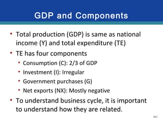
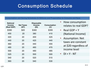
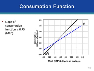
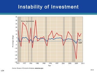
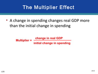
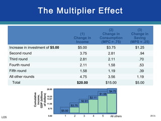
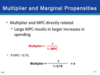
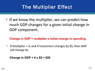
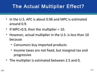
Chapter 28
Basic Macroeconomic
Relationships
Copyright © 2015 McGraw-Hill Education. All rights reserved. No reproduction or distribution without the prior written consent of McGraw-Hill Education.
28-2
GDP and Components
• Total production (GDP) is same as national
income (Y) and total expenditure (TE)
• TE has four components
• Consumption (C): 2/3 of GDP
• Investment (I): Irregular
• Government purchases (G)
• Net exports (NX): Mostly negative
• To understand business cycle, it is important
to understand how they are related.
28-3
Basic Macroeconomic
Relationships
• Three basic macroeconomic relationships
• Consumption and Income
• Consumption and saving
• Interest rate and Investment
• Spending and Output
• Multiplier effect
28-4
• National Income (Y): total income earned by
households equal to GDP
• Net taxes: Taxes minus transfer payments
• NT = Taxes – Transfer payments
• Disposable Income: Income after taxes and
transfer payments
• DI = Y – NT
National Income and Disposable
Income
LO1
28-5
• Disposable Income can be freely spent
(consumption) or saved (saving) by
households.
• DI = C + S
• Disposable Income and Consumption
• When C < DI, S > 0 (Saving)
• When C > DI, S < 0 (Dis-saving)
Income, Consumption, and Saving
LO1
28-6
• Consumption schedule
• Disposable income is the major determinant
of consumption
• Relationship between Disposable income and
consumption
• Higher the disposable income, higher the
consumption.
Income, Consumption, and Saving
LO1
28-7
Income Consumption and Saving
LO1
28-8
Marginal Propensity to Consume
• Marginal propensity to consume (MPC)
• Proportion of a change in income consumed
• Because households spends only fraction of
disposable income and save the rest, MPC is
less than 1.
MPC = =
change in consumption
change in income ΔDI
ΔC
LO1
28-9
Marginal Propensities
Disposable income
Consumption
C
MPC =
15
20 = .75
∆C ($15)
∆DI ($20)
• MPC=0.75 means
• 75% of additional
income will be spent.
• When household’s
disposable income
increases by $1, the
house hold will spend
75¢ portion of
additional $1 income.
• It is also a slope of
consumption function.
28-10
Average Propensities
• Average propensity to consume (APC)
• Fraction of total income consumed
• Average propensity to save (APS): Saving rate
• Fraction of total income saved
APC = APS =
consumption
income income
saving
APC + APS = 1
LO1
28-11
Global Perspective
LO1
28-12
Consumption Schedule
Consumption and Saving Schedules (in Billions) and Propensities to Consume and Save
Disposable
Income
(DI)
Consumption
(C)
Saving
(S)
$360 $395
380 410
400 425
420 440
440 455
460 470
480 485
500 500
520 515
540 530
LO1
Consumption and Saving Schedules (in Billions) and Propensities to Consume and Save
Disposable
Income
(DI)
Consumption
(C)
Saving
(S)
Change in
Disposable
Income
(∆DI)
Change in
Consumption
(∆C)
$360 $395 $-35
380 410 -30
400 425 -25
420 440 -20
440 455 -15
460 470 -10
480 485 -5
500 500 0
520 515 5
540 530 10
Consumption and Saving Schedules (in Billions) and Propensities to Consume and Save
Disposable
Income
(DI)
Consumption
(C)
Saving
(S)
Change in
Disposable
Income
(∆DI)
Change in
Consumption
(∆C)
Marginal
Propensity to
Consume
(MPC)
$360 $395 $-35
380 410 -30 $20 $15
400 425 -25 $20 $15
420 440 -20 $20 $15
440 455 -15 $20 $15
460 470 -10 $20 $15
480 485 -5 $20 $15
500 500 0 $20 $15
520 515 5 $20 $15
540 530 10 $20 $15
Consumption and Saving Schedules (in Billions) and Propensities to Consume and Save
Disposable
Income
(DI)
Consumption
(C)
Saving
(S)
Change in
Disposable
Income
(∆DI)
Change in
Consumption
(∆C)
Marginal
Propensity to
Consume
(MPC)
$360 $395 $-35
380 410 -30 $20 $15 .75
400 425 -25 $20 $15 .75
420 440 -20 $20 $15 .75
440 455 -15 $20 $15 .75
460 470 -10 $20 $15 .75
480 485 -5 $20 $15 .75
500 500 0 $20 $15 .75
520 515 5 $20 $15 .75
540 530 10 $20 $15 .75
28-13
Consumption Function
400 420 440 460 480 500 520 540
C
Consumption
functionSaving $5 billion
Dissaving $10 billion
Consumption(billionsofdollars)
Disposable income (billions of dollars)
28-14
Determinants Of Consumption
• Amount of disposable income is the main
determinant
• Other determinants
• Wealth: Wealth↑ → Consumption↑
• Expectations:
Income Expectation↑ → Consumption↑
• Real interest rates: Affect an amount of
borrowings and savings, which affect consumption
Real interest rates↑ → Borrowings↓ & Savings↑
→ Consumption↓
LO2
28-15
Consumption and Saving Schedules (in Billions) and Propensities to Consume and Save
National
Income
(Real GDP)
Net Taxes
(NT)
$380
400
420
440
460
480
500
520
540
560
Consumption Schedule
LO1
Consumption and Saving Schedules (in Billions) and Propensities to Consume and Save
National
Income
(Real GDP)
Net Taxes
(NT)
Disposable
Income
(DI)
$380 $20
400 20
420 20
440 20
460 20
480 20
500 20
520 20
540 20
560 20
Consumption and Saving Schedules (in Billions) and Propensities to Consume and Save
National
Income
(Real GDP)
Net Taxes
(NT)
Disposable
Income
(DI)
Consumption
(C)
$380 $20 $360
400 20 380
420 20 400
440 20 420
460 20 440
480 20 460
500 20 480
520 20 500
540 20 520
560 20 540
Consumption and Saving Schedules (in Billions) and Propensities to Consume and Save
National
Income
(Real GDP)
Net Taxes
(NT)
Disposable
Income
(DI)
Consumption
(C)
$380 $20 $360 $395
400 20 380 410
420 20 400 425
440 20 420 440
460 20 440 455
480 20 460 470
500 20 480 485
520 20 500 500
540 20 520 515
560 20 540 530
• How consumption
relates to real GDP?
• Real GDP = Y
(National Income)
• Assumption: Net
taxes are constant
at $20 regardless of
income level
• DI = Y - NT
28-16
Consumption Function
C0
Real GDP (billions of dollars)
Consumption
(billionsofdollars)
• Slope of
consumption
function is 0.75
(MPC).
400 420 440 460 480 500 520 540
520
500
480
460
440
420
400
28-17
Changes in Consumption Schedule
• When the determinant of consumption
changes, the consumption function shifts
• Wealth↑ → Consumption function ↑
• Income Expectation↑ → Consumption function↑
• Real interest rates↑ → Consumption function↓
LO2
28-18
Shifts of C & S Schedules
C0
Real GDP (billions of dollars)
Consumption
(billionsofdollars)
C2
C1
0
Increase in consumption:
Consumption function
shifts up (↑).
Decrease in consumption:
Consumption function
shifts down (↓).
28-19
• Investment: Firms’ spending on new plants,
equipment, machinery, and tools
• Firm’s investment depends on
• Expected rate of return on investment project:
Expected rate of return ↑ → investment ↑
• Real interest rate:
• Investment projects are financed by borrowing
• Real interest rate on borrowing is the
opportunity cost of investment
Interest-Rate-Investment
Relationship
LO3
28-20
• Investment demand: A relationship between
the real interest rate and Investment
• Real interest rate ↑ → investment ↓
• Investment demand curve is downward-sloping.
Investment Demand
LO3
28-21
Investment Demand Curve
I
Real
Interest
Rate
Investment
(billions
of dollars)
16% $ 0
14 5
12 10
10 15
8 20
6 25
4 30
2 35
0 40
Investment
demand
curve
LO3
28-22
Shifts of Investment Demand
• Investment demand changes when changes in
• Business taxes↑ → investment ↓
• Technological change↑ → investment ↑
• Expectations
• Expected return↑ → investment ↑
• Expected risk↑ → investment ↓
LO4
28-23
Shifts of Investment Demand
Realinterestrate(percent)
0 Investment (billions of dollars)
ID0
ID1ID2
Increase
in investment
demand
Decrease in
investment
demand
LO4
28-24
Global Perspective
LO4
28-25
Instability of Investment
• Investment demand is volatile due to
• Variability of expectations
• Variability of profits
• Both expectations and profits change along the
business cycle
• Optimistic expectations and high profits during
expansions, while pessimistic expectations and low
profits during recessions.
• Irregularity of innovation
LO4
28-26
Instability of Investment
LO4
28-27
Investment and GDP
• Investment spending changes erratically
• Investment spending fluctuates much more
than GDP
• When Investment spending is down (up), GDP
is also down (up).
• Investment spending downturns correspond
to recessions.
LO4
28-28
The Multiplier Process
• When one of components of GDP changes, GDP also
changes.
Y = C + I + G + NX
• Then, a change in GDP (national Income) causes a
change in consumption.
• A change in consumption further changes GDP.
• …
• Eventually, GDP will change more than an initial
change in one component which started the
multiplier process.
LO5
28-29
The Multiplier Process
The initial increase in
investment ($5.00)
brought an even
bigger increase in real
GDP because it
induced an increase in
consumption
expenditure.
LO5
I↑ by $5.00 ⇒ GDP↑ by $5.00 ⇒ Y↑ by $5.00
⇒ C↑ by $3.75 ⇒ GDP↑ by $3.75 ⇒ Y↑ by $3.75
⇒ C↑ by $2.81 …..
28-30
The Multiplier Effect
• A change in spending changes real GDP more
than the initial change in spending
Multiplier =
change in real GDP
initial change in spending
LO5
28-31
The Multiplier Effect
(1)
Change in
Income
(2)
Change in
Consumption
(MPC = .75)
(3)
Change in
Saving
(MPS = .25)
Increase in investment of $5.00 $5.00 $3.75 $1.25
Second round 3.75 2.81 .94
Third round 2.81 2.11 .70
Fourth round 2.11 1.58 .53
Fifth round 1.58 1.19 .39
All other rounds 4.75 3.56 1.19
Total $20.00 $15.00 $5.00
$5.00
$3.75
$2.81
$2.11
$1.58
$4.75
Cumulative
income,
GDP(billions
ofdollars)
20.00
15.25
13.67
11.56
8.75
5.00 2 3 54 All others1
LO5
28-32
Multiplier and Marginal Propensities
• Multiplier and MPC directly related
• Large MPC results in larger increases in
spending
Multiplier =
1
1- MPC
LO5
• If MPC = 0.75,
Multiplier =
1
1- 0.75
= 4
28-33
The Multiplier Effect
• If we know the multiplier, we can predict how
much GDP changes for a given initial change in
GDP component.
Change in GDP = multiplier x initial change in spending
LO5
• If Multiplier = 4, and if Investment changes by $5, then GDP
will change by
Change in GDP = 4 x $5 = $20
28-34
The Actual Multiplier Effect?
• In the U.S. APC is about 0.96 and MPC is estimated
around 0.9.
• If MPC=0.9, then the multiplier = 10.
• However, actual multiplier in the U.S. is less than 10
because
• Consumers buy imported products
• Income taxes are not fixed, but marginal tax and
progressive
• The multiplier is estimated between 2.5 and 0.
LO5
28-35
Investment and Economy
• Even though Investment is a small portion of GDP, its
irregular changes have multiplier effect on GDP of
economy.
• When entrepreneurs become pessimistic, they cut
investment spending
• Creates a ripple effect of people not spending,
following the first decision
• Ultimately the entire economy experiences an
economic downturn – recession
• Business cycles are result of irregular changes in
Investment and other components of GDP

Econ789 chapter028

  • 1.
    Chapter 28 Basic Macroeconomic Relationships Copyright© 2015 McGraw-Hill Education. All rights reserved. No reproduction or distribution without the prior written consent of McGraw-Hill Education.
  • 2.
    28-2 GDP and Components •Total production (GDP) is same as national income (Y) and total expenditure (TE) • TE has four components • Consumption (C): 2/3 of GDP • Investment (I): Irregular • Government purchases (G) • Net exports (NX): Mostly negative • To understand business cycle, it is important to understand how they are related.
  • 3.
    28-3 Basic Macroeconomic Relationships • Threebasic macroeconomic relationships • Consumption and Income • Consumption and saving • Interest rate and Investment • Spending and Output • Multiplier effect
  • 4.
    28-4 • National Income(Y): total income earned by households equal to GDP • Net taxes: Taxes minus transfer payments • NT = Taxes – Transfer payments • Disposable Income: Income after taxes and transfer payments • DI = Y – NT National Income and Disposable Income LO1
  • 5.
    28-5 • Disposable Incomecan be freely spent (consumption) or saved (saving) by households. • DI = C + S • Disposable Income and Consumption • When C < DI, S > 0 (Saving) • When C > DI, S < 0 (Dis-saving) Income, Consumption, and Saving LO1
  • 6.
    28-6 • Consumption schedule •Disposable income is the major determinant of consumption • Relationship between Disposable income and consumption • Higher the disposable income, higher the consumption. Income, Consumption, and Saving LO1
  • 7.
  • 8.
    28-8 Marginal Propensity toConsume • Marginal propensity to consume (MPC) • Proportion of a change in income consumed • Because households spends only fraction of disposable income and save the rest, MPC is less than 1. MPC = = change in consumption change in income ΔDI ΔC LO1
  • 9.
    28-9 Marginal Propensities Disposable income Consumption C MPC= 15 20 = .75 ∆C ($15) ∆DI ($20) • MPC=0.75 means • 75% of additional income will be spent. • When household’s disposable income increases by $1, the house hold will spend 75¢ portion of additional $1 income. • It is also a slope of consumption function.
  • 10.
    28-10 Average Propensities • Averagepropensity to consume (APC) • Fraction of total income consumed • Average propensity to save (APS): Saving rate • Fraction of total income saved APC = APS = consumption income income saving APC + APS = 1 LO1
  • 11.
  • 12.
    28-12 Consumption Schedule Consumption andSaving Schedules (in Billions) and Propensities to Consume and Save Disposable Income (DI) Consumption (C) Saving (S) $360 $395 380 410 400 425 420 440 440 455 460 470 480 485 500 500 520 515 540 530 LO1 Consumption and Saving Schedules (in Billions) and Propensities to Consume and Save Disposable Income (DI) Consumption (C) Saving (S) Change in Disposable Income (∆DI) Change in Consumption (∆C) $360 $395 $-35 380 410 -30 400 425 -25 420 440 -20 440 455 -15 460 470 -10 480 485 -5 500 500 0 520 515 5 540 530 10 Consumption and Saving Schedules (in Billions) and Propensities to Consume and Save Disposable Income (DI) Consumption (C) Saving (S) Change in Disposable Income (∆DI) Change in Consumption (∆C) Marginal Propensity to Consume (MPC) $360 $395 $-35 380 410 -30 $20 $15 400 425 -25 $20 $15 420 440 -20 $20 $15 440 455 -15 $20 $15 460 470 -10 $20 $15 480 485 -5 $20 $15 500 500 0 $20 $15 520 515 5 $20 $15 540 530 10 $20 $15 Consumption and Saving Schedules (in Billions) and Propensities to Consume and Save Disposable Income (DI) Consumption (C) Saving (S) Change in Disposable Income (∆DI) Change in Consumption (∆C) Marginal Propensity to Consume (MPC) $360 $395 $-35 380 410 -30 $20 $15 .75 400 425 -25 $20 $15 .75 420 440 -20 $20 $15 .75 440 455 -15 $20 $15 .75 460 470 -10 $20 $15 .75 480 485 -5 $20 $15 .75 500 500 0 $20 $15 .75 520 515 5 $20 $15 .75 540 530 10 $20 $15 .75
  • 13.
    28-13 Consumption Function 400 420440 460 480 500 520 540 C Consumption functionSaving $5 billion Dissaving $10 billion Consumption(billionsofdollars) Disposable income (billions of dollars)
  • 14.
    28-14 Determinants Of Consumption •Amount of disposable income is the main determinant • Other determinants • Wealth: Wealth↑ → Consumption↑ • Expectations: Income Expectation↑ → Consumption↑ • Real interest rates: Affect an amount of borrowings and savings, which affect consumption Real interest rates↑ → Borrowings↓ & Savings↑ → Consumption↓ LO2
  • 15.
    28-15 Consumption and SavingSchedules (in Billions) and Propensities to Consume and Save National Income (Real GDP) Net Taxes (NT) $380 400 420 440 460 480 500 520 540 560 Consumption Schedule LO1 Consumption and Saving Schedules (in Billions) and Propensities to Consume and Save National Income (Real GDP) Net Taxes (NT) Disposable Income (DI) $380 $20 400 20 420 20 440 20 460 20 480 20 500 20 520 20 540 20 560 20 Consumption and Saving Schedules (in Billions) and Propensities to Consume and Save National Income (Real GDP) Net Taxes (NT) Disposable Income (DI) Consumption (C) $380 $20 $360 400 20 380 420 20 400 440 20 420 460 20 440 480 20 460 500 20 480 520 20 500 540 20 520 560 20 540 Consumption and Saving Schedules (in Billions) and Propensities to Consume and Save National Income (Real GDP) Net Taxes (NT) Disposable Income (DI) Consumption (C) $380 $20 $360 $395 400 20 380 410 420 20 400 425 440 20 420 440 460 20 440 455 480 20 460 470 500 20 480 485 520 20 500 500 540 20 520 515 560 20 540 530 • How consumption relates to real GDP? • Real GDP = Y (National Income) • Assumption: Net taxes are constant at $20 regardless of income level • DI = Y - NT
  • 16.
    28-16 Consumption Function C0 Real GDP(billions of dollars) Consumption (billionsofdollars) • Slope of consumption function is 0.75 (MPC). 400 420 440 460 480 500 520 540 520 500 480 460 440 420 400
  • 17.
    28-17 Changes in ConsumptionSchedule • When the determinant of consumption changes, the consumption function shifts • Wealth↑ → Consumption function ↑ • Income Expectation↑ → Consumption function↑ • Real interest rates↑ → Consumption function↓ LO2
  • 18.
    28-18 Shifts of C& S Schedules C0 Real GDP (billions of dollars) Consumption (billionsofdollars) C2 C1 0 Increase in consumption: Consumption function shifts up (↑). Decrease in consumption: Consumption function shifts down (↓).
  • 19.
    28-19 • Investment: Firms’spending on new plants, equipment, machinery, and tools • Firm’s investment depends on • Expected rate of return on investment project: Expected rate of return ↑ → investment ↑ • Real interest rate: • Investment projects are financed by borrowing • Real interest rate on borrowing is the opportunity cost of investment Interest-Rate-Investment Relationship LO3
  • 20.
    28-20 • Investment demand:A relationship between the real interest rate and Investment • Real interest rate ↑ → investment ↓ • Investment demand curve is downward-sloping. Investment Demand LO3
  • 21.
    28-21 Investment Demand Curve I Real Interest Rate Investment (billions ofdollars) 16% $ 0 14 5 12 10 10 15 8 20 6 25 4 30 2 35 0 40 Investment demand curve LO3
  • 22.
    28-22 Shifts of InvestmentDemand • Investment demand changes when changes in • Business taxes↑ → investment ↓ • Technological change↑ → investment ↑ • Expectations • Expected return↑ → investment ↑ • Expected risk↑ → investment ↓ LO4
  • 23.
    28-23 Shifts of InvestmentDemand Realinterestrate(percent) 0 Investment (billions of dollars) ID0 ID1ID2 Increase in investment demand Decrease in investment demand LO4
  • 24.
  • 25.
    28-25 Instability of Investment •Investment demand is volatile due to • Variability of expectations • Variability of profits • Both expectations and profits change along the business cycle • Optimistic expectations and high profits during expansions, while pessimistic expectations and low profits during recessions. • Irregularity of innovation LO4
  • 26.
  • 27.
    28-27 Investment and GDP •Investment spending changes erratically • Investment spending fluctuates much more than GDP • When Investment spending is down (up), GDP is also down (up). • Investment spending downturns correspond to recessions. LO4
  • 28.
    28-28 The Multiplier Process •When one of components of GDP changes, GDP also changes. Y = C + I + G + NX • Then, a change in GDP (national Income) causes a change in consumption. • A change in consumption further changes GDP. • … • Eventually, GDP will change more than an initial change in one component which started the multiplier process. LO5
  • 29.
    28-29 The Multiplier Process Theinitial increase in investment ($5.00) brought an even bigger increase in real GDP because it induced an increase in consumption expenditure. LO5 I↑ by $5.00 ⇒ GDP↑ by $5.00 ⇒ Y↑ by $5.00 ⇒ C↑ by $3.75 ⇒ GDP↑ by $3.75 ⇒ Y↑ by $3.75 ⇒ C↑ by $2.81 …..
  • 30.
    28-30 The Multiplier Effect •A change in spending changes real GDP more than the initial change in spending Multiplier = change in real GDP initial change in spending LO5
  • 31.
    28-31 The Multiplier Effect (1) Changein Income (2) Change in Consumption (MPC = .75) (3) Change in Saving (MPS = .25) Increase in investment of $5.00 $5.00 $3.75 $1.25 Second round 3.75 2.81 .94 Third round 2.81 2.11 .70 Fourth round 2.11 1.58 .53 Fifth round 1.58 1.19 .39 All other rounds 4.75 3.56 1.19 Total $20.00 $15.00 $5.00 $5.00 $3.75 $2.81 $2.11 $1.58 $4.75 Cumulative income, GDP(billions ofdollars) 20.00 15.25 13.67 11.56 8.75 5.00 2 3 54 All others1 LO5
  • 32.
    28-32 Multiplier and MarginalPropensities • Multiplier and MPC directly related • Large MPC results in larger increases in spending Multiplier = 1 1- MPC LO5 • If MPC = 0.75, Multiplier = 1 1- 0.75 = 4
  • 33.
    28-33 The Multiplier Effect •If we know the multiplier, we can predict how much GDP changes for a given initial change in GDP component. Change in GDP = multiplier x initial change in spending LO5 • If Multiplier = 4, and if Investment changes by $5, then GDP will change by Change in GDP = 4 x $5 = $20
  • 34.
    28-34 The Actual MultiplierEffect? • In the U.S. APC is about 0.96 and MPC is estimated around 0.9. • If MPC=0.9, then the multiplier = 10. • However, actual multiplier in the U.S. is less than 10 because • Consumers buy imported products • Income taxes are not fixed, but marginal tax and progressive • The multiplier is estimated between 2.5 and 0. LO5
  • 35.
    28-35 Investment and Economy •Even though Investment is a small portion of GDP, its irregular changes have multiplier effect on GDP of economy. • When entrepreneurs become pessimistic, they cut investment spending • Creates a ripple effect of people not spending, following the first decision • Ultimately the entire economy experiences an economic downturn – recession • Business cycles are result of irregular changes in Investment and other components of GDP

Editor's Notes

  • #2 This chapter introduces three basic macroeconomic relationships. First, the focus is on the income-consumption and income-saving relationships. Second, the relationship between the interest rate and investment is examined. Finally, the multiplier concept is developed, relating changes in spending to changes in output.
  • #5 DI represents disposable income (after-tax income) and is the most important determinant of C (consumption spending). What is not spent is called saving. Both consumption and saving are directly related to the level of income. We can make the following conclusions: Households consume a large portion of their disposable income and spend a larger proportion of a small disposable income than of a large disposable income. Households save a smaller proportion of a small disposable income than of a large disposable income. Dissaving is consuming in excess of disposable income. Households dissave by borrowing or by selling accumulated wealth (assets).
  • #6 DI represents disposable income (after-tax income) and is the most important determinant of C (consumption spending). What is not spent is called saving. Both consumption and saving are directly related to the level of income. We can make the following conclusions: Households consume a large portion of their disposable income and spend a larger proportion of a small disposable income than of a large disposable income. Households save a smaller proportion of a small disposable income than of a large disposable income. Dissaving is consuming in excess of disposable income. Households dissave by borrowing or by selling accumulated wealth (assets).
  • #7 DI represents disposable income (after-tax income) and is the most important determinant of C (consumption spending). What is not spent is called saving. Both consumption and saving are directly related to the level of income. We can make the following conclusions: Households consume a large portion of their disposable income and spend a larger proportion of a small disposable income than of a large disposable income. Households save a smaller proportion of a small disposable income than of a large disposable income. Dissaving is consuming in excess of disposable income. Households dissave by borrowing or by selling accumulated wealth (assets).
  • #8 This figure shows the consumption and disposable income for the U.S. for 1987–2012. Each dot in this figure shows consumption and disposable income in a specific year. The line, C, which generalizes the relationship between consumption and disposable income, indicates a direct relationship and shows that households consume most of their after-tax incomes. This figure represents graphically the recent historical relationship between disposable income (DI), consumption (C), and saving (S) in the United States. A 45-degree line represents all points where consumer spending is equal to disposable income. Other points represent actual C, DI relationships for each year. If the actual graph of the relationship between consumption and income is below the 45-degree line, then the difference must represent the amount of income that is saved. Notice that consumption can exceed disposable income and personal saving can be negative.
  • #9 Marginal propensity to consume (MPC) is the fraction or proportion of any change in income that is consumed. (MPC = change in consumption/change in income.) Marginal propensity to save (MPS) is the fraction or proportion of any change in income that is saved. (MPS = change in saving/change in income.) Note that MPC + MPS = 1.
  • #10 This figure shows the marginal propensity to consume and the marginal propensity to save as the slopes of the consumption and savings schedules. The MPC is the slope of the consumption schedule and the MPS is the slope of the saving schedule. The Greek letter delta means “the change in.”
  • #11 The definition of the average propensity to consume (APC) is the fraction, or percentage, of income consumed (APC = consumption/income). If you multiply the fraction by 100 you can express this as a percentage. The definition of the average propensity to save (APS) is a the fraction, or percentage, of income saved (APS = saving/income). If you multiply the fraction by 100 you can express this as a percentage. The Global Perspective shows the APCs for several nations in 2009. Note the high APCs for Australia, the U.S., and Canada. Note that APC + APS = 1.
  • #12 This Global Perspective shows the average propensities to consume for selected nations. There are surprisingly large differences in the average propensities to consume (APCs) among nations. In 2011, Canada and the United States, in particular, had substantially higher APCs, and thus lower APSs, than several other advanced economies.
  • #13 This table shows the consumption and saving schedules and propensities to consume and save (propensities to consume and save will be presented in later slides). A hypothetical consumption schedule shows that households spend a larger proportion of a small income than of a large income based on the APC. Note that “dissaving” occurs at low levels of disposable income, where consumption exceeds income and households must borrow or use up some of their wealth. The break-even income is where C= DI and S= 0. In this table, the break-even income occurs when DI = $390.
  • #14 This figure shows (a) consumption and (b) saving schedules. The two parts of this figure show the income-consumption and income-saving relationships graphically. The saving schedule in (b) is found by subtracting the consumption schedule in (a) vertically from the 45° line. Consumption equals disposable income (and saving, thus, equals zero) at $390 billion for this hypothetical data.
  • #15 Nonincome determinants of consumption and saving can cause people to spend or save more or less at various income levels, although the level of income is the basic determinant. Wealth: An increase in wealth shifts the consumption schedule up and the saving schedule down. In recent years, major fluctuations in stock market values have increased the importance of this wealth effect. A “reverse wealth effect” occurred in 2000 and 2001 when stock prices fell dramatically. Household debt: Lower debt levels shift the consumption schedule up and the saving schedule down. Expectations: Changes in expected future prices or wealth can affect consumption spending today. Real interest rates: Declining interest rates increase the incentive to borrow and consume, and reduce the incentive to save. Because many household expenditures are not interest sensitive – the electric bill, groceries, etc. – the effect of interest rate changes on spending are modest.
  • #16 This table shows the consumption and saving schedules and propensities to consume and save (propensities to consume and save will be presented in later slides). A hypothetical consumption schedule shows that households spend a larger proportion of a small income than of a large income based on the APC. Note that “dissaving” occurs at low levels of disposable income, where consumption exceeds income and households must borrow or use up some of their wealth. The break-even income is where C= DI and S= 0. In this table, the break-even income occurs when DI = $390.
  • #17 This figure shows the shifts of the consumption and saving schedules. Normally, if households consume more at each level of real GDP, they are necessarily saving less. Graphically this means that an upward shift of the consumption schedule (C0 to C1) entails a downward shift of the saving schedule (S0 to S1). If households consume less at each level of real GDP, they are saving more. A downward shift of the consumption schedule (C0 to C2) is reflected in an upward shift of the saving schedule (S0 to S2). This pattern breaks down, however, when taxes change; then the consumption and saving schedules move in the same direction—opposite to the direction of the tax change.
  • #18 Macroeconomic models focus on real domestic output (real GDP) more than on disposable income. The figure on the next slide reflects this change in the labeling of the horizontal axis. Changes along schedules: Movement from one point to another on a given schedule is called a change in the amount consumed. A shift in the schedule is called a change in the consumption schedule and is caused by one of the non-income determinants of consumption. Schedule shifts: Consumption and saving schedules will always shift in opposite directions unless a shift is caused by a tax change. Taxation: Lower taxes will shift both schedules up since taxation affects both spending and saving and vice versa for higher taxes. Stability: Economists believe that the consumption and saving schedules are generally stable unless deliberately shifted by government action.
  • #19 This figure shows the shifts of the consumption and saving schedules. Normally, if households consume more at each level of real GDP, they are necessarily saving less. Graphically this means that an upward shift of the consumption schedule (C0 to C1) entails a downward shift of the saving schedule (S0 to S1). If households consume less at each level of real GDP, they are saving more. A downward shift of the consumption schedule (C0 to C2) is reflected in an upward shift of the saving schedule (S0 to S2). This pattern breaks down, however, when taxes change; then the consumption and saving schedules move in the same direction—opposite to the direction of the tax change.
  • #20 Investment consists of spending on new plants, capital equipment, machinery, inventories, construction, etc. The investment decision weighs marginal benefits and marginal costs. The expected rate of return is the marginal benefit and the interest rate (the cost of borrowing funds) represents the marginal cost. The expected rate of return is found by finding the expected economic profit (total revenue minus total cost) as a percentage of the cost of investment. The text’s example gives $100 expected profit on a $1000 investment, for a 10% expected rate of return. Thus, the business would not want to pay more than a 10% interest rate on the investment. Remember that the expected rate of return is not a guaranteed rate of return. Investment carries risk. The real interest rate, i (nominal rate corrected for expected inflation), determines the cost of investment. The interest rate represents either the cost of borrowed funds or the opportunity cost of investing your own funds, which is income forgone. If the real interest rate exceeds the expected rate of return, the investment should not be made. The investment demand schedule, or curve, shows an inverse relationship between the interest rate and the amount of investment. As long as the expected return exceeds the interest rate, the investment is expected to be profitable.
  • #21 Investment consists of spending on new plants, capital equipment, machinery, inventories, construction, etc. The investment decision weighs marginal benefits and marginal costs. The expected rate of return is the marginal benefit and the interest rate (the cost of borrowing funds) represents the marginal cost. The expected rate of return is found by finding the expected economic profit (total revenue minus total cost) as a percentage of the cost of investment. The text’s example gives $100 expected profit on a $1000 investment, for a 10% expected rate of return. Thus, the business would not want to pay more than a 10% interest rate on the investment. Remember that the expected rate of return is not a guaranteed rate of return. Investment carries risk. The real interest rate, i (nominal rate corrected for expected inflation), determines the cost of investment. The interest rate represents either the cost of borrowed funds or the opportunity cost of investing your own funds, which is income forgone. If the real interest rate exceeds the expected rate of return, the investment should not be made. The investment demand schedule, or curve, shows an inverse relationship between the interest rate and the amount of investment. As long as the expected return exceeds the interest rate, the investment is expected to be profitable.
  • #22 This figure, which can be found in the Key Graph section, shows the investment demand curve. The investment demand curve is constructed by arraying all potential investment projects in descending order of their expected rates of return. The curve slopes downward, reflecting an inverse relationship between the real interest rate (the financial “price” of each dollar of investing) and the quantity of investment demanded.
  • #23 Shifts in investment demand (see the next slide for the figure that represents the graph) occur when any determinant apart from the interest rate changes. Greater expected returns create more investment demand, shifting the curve to the right. The reverse causes a leftward shift. Changes in expected returns result because: Acquisition, maintenance, and operating costs of capital goods may change. Higher costs lower the expected return. Business taxes may change. Increased taxes lower the expected return. Technology may change. Technological change often involves lower costs, which would increase expected returns. Stock of capital goods on hand will affect new investment. If there is abundant idle capital on hand because of weak demand or recent investment, new investments would be less profitable. If firms are planning on increasing their inventories, investment demand shifts to the right. If firms are planning to decrease their inventories, investment demand shifts left. These planned inventory changes are based on expectations of either faster or slower sales. If the firm expects faster sales in the future, they will add to inventory. If the firm expects slower sales in the future, they will decrease inventories. Expectations about future economic and political conditions, both in the aggregate and in certain specific markets, can change the view of expected profits.
  • #24 This figure shows the shifts of the investment demand curve. Increases in investment demand are shown as rightward shifts of the investment demand curve; decreases in investment demand are shown as leftward shifts of the investment demand curve.
  • #25 This Global Perspective shows gross investment expenditures as a percentage of GDP for selected nations for 2011. As a percentage of GDP, investment varies widely by nation. These differences, of course, can change from year to year.
  • #26 Investment is a very unstable type of spending. Ig is more volatile than GDP. Expectations of future business conditions are easily and quickly changed. Capital goods are durable, so spending can be postponed or not. Firms can choose to replace or fix older equipment and buildings. This is unpredictable. Innovation occurs irregularly; new products stimulate investment and create waves of investment spending that in time recede. Profits affect both the incentive and ability to invest and profits vary considerably from year-to-year, contributing to the instability of investment spending.
  • #27 This figure shows the volatility of investment for the period 1973–2012. Annual percentage changes in investment spending are often several times greater than the percentage changes in GDP. (Data is represented in real terms. Investment is gross private domestic investment).
  • #28 Investment is a very unstable type of spending. Ig is more volatile than GDP. Expectations of future business conditions are easily and quickly changed. Capital goods are durable, so spending can be postponed or not. Firms can choose to replace or fix older equipment and buildings. This is unpredictable. Innovation occurs irregularly; new products stimulate investment and create waves of investment spending that in time recede. Profits affect both the incentive and ability to invest and profits vary considerably from year-to-year, contributing to the instability of investment spending.
  • #29 Changes in spending ripple through the economy to generate even larger changes in real GDP. This is called the multiplier effect. Multiplier = change in real GDP / initial change in spending. Alternatively, it can be rearranged to read: change in real GDP = initial change in spending x multiplier. Points to remember about the multiplier: The initial change in spending is usually associated with investment because it is so volatile, but changes in consumption (unrelated to income), net exports, and government purchases also are subject to the multiplier effect. The initial change refers to an up-shift or down-shift in the aggregate expenditures schedule due to a change in one of its components, like investment. The multiplier works in both directions (up or down). It occurs because of the interconnectedness of the economy.
  • #30 Changes in spending ripple through the economy to generate even larger changes in real GDP. This is called the multiplier effect. Multiplier = change in real GDP / initial change in spending. Alternatively, it can be rearranged to read: change in real GDP = initial change in spending x multiplier. Points to remember about the multiplier: The initial change in spending is usually associated with investment because it is so volatile, but changes in consumption (unrelated to income), net exports, and government purchases also are subject to the multiplier effect. The initial change refers to an up-shift or down-shift in the aggregate expenditures schedule due to a change in one of its components, like investment. The multiplier works in both directions (up or down). It occurs because of the interconnectedness of the economy.
  • #31 Changes in spending ripple through the economy to generate even larger changes in real GDP. This is called the multiplier effect. Multiplier = change in real GDP / initial change in spending. Alternatively, it can be rearranged to read: change in real GDP = initial change in spending x multiplier. Points to remember about the multiplier: The initial change in spending is usually associated with investment because it is so volatile, but changes in consumption (unrelated to income), net exports, and government purchases also are subject to the multiplier effect. The initial change refers to an up-shift or down-shift in the aggregate expenditures schedule due to a change in one of its components, like investment. The multiplier works in both directions (up or down). It occurs because of the interconnectedness of the economy.
  • #32 This figure illustrates the multiplier process with an MPC of .75. An initial change in investment spending of $5 billion creates an equal $5 billion of new income in round 1. Households spend $3.75 billion of this new income, creating $3.75 of added income in round 2. Of this $3.75 of new income, households spend $2.81 billion, and income rises by that amount in round 3. Such income increments over the entire process get successively smaller but eventually produce a total change of income and GDP of $20 billion. The multiplier therefore is 4.
  • #33 The significance of the multiplier is that a small change in investment plans or consumption-saving plans can trigger a much larger change in the equilibrium level of GDP. The magnitude of the change in GDP is dependent on the size of the MPC and MPS.
  • #34 Changes in spending ripple through the economy to generate even larger changes in real GDP. This is called the multiplier effect. Multiplier = change in real GDP / initial change in spending. Alternatively, it can be rearranged to read: change in real GDP = initial change in spending x multiplier. Points to remember about the multiplier: The initial change in spending is usually associated with investment because it is so volatile, but changes in consumption (unrelated to income), net exports, and government purchases also are subject to the multiplier effect. The initial change refers to an up-shift or down-shift in the aggregate expenditures schedule due to a change in one of its components, like investment. The multiplier works in both directions (up or down). It occurs because of the interconnectedness of the economy.
  • #35 The actual multiplier in the U.S. (estimated to be between 2.5 and 0) is smaller than the model in this chapter because, in the U.S. economy, there are other leakages from the spending and income cycle besides just saving. Imports and taxes reduce the flow of money back into spending on domestically produced output, reducing the multiplier effect. Also, increases in spending can drive up prices (inflation) and at higher prices, any given amount of spending will buy less real output.
  • #36 The central idea illustrated in this example is of the multiplier effect that exists in a market economic system. One independently determined change in spending has an effect on another’s income, which then sets in motion a chain of events whereby spending changes directly with the income changes. A decline in spending begins a chain of declines, or, in other words, the initial decrease in spending is multiplied in terms of the final effect of this single decision. This occurs because of the observation that any change in income causes a change in spending that is directly proportional to it. The multiplier effect helps us understand why there is a business cycle as opposed to a stable level of output growth from year to year. In the Buchwald piece, a “downturn” for one person became a downturn for everyone in that fictional economy. Likewise, if the story had begun with a burst of optimism and an increase in spending, it might have rippled through to expand everyone’s fortunes. The multiplier intensifies the effect of a spending change, whether it is an increase or decrease. The multiplier is based on two facts: 1. The economy has continuous flows of expenditures and income—a ripple effect—in which income received by one comes from money spent by another, and so forth. 2. Any change in income will cause both consumption and saving to vary in the same direction as the initial change in income.