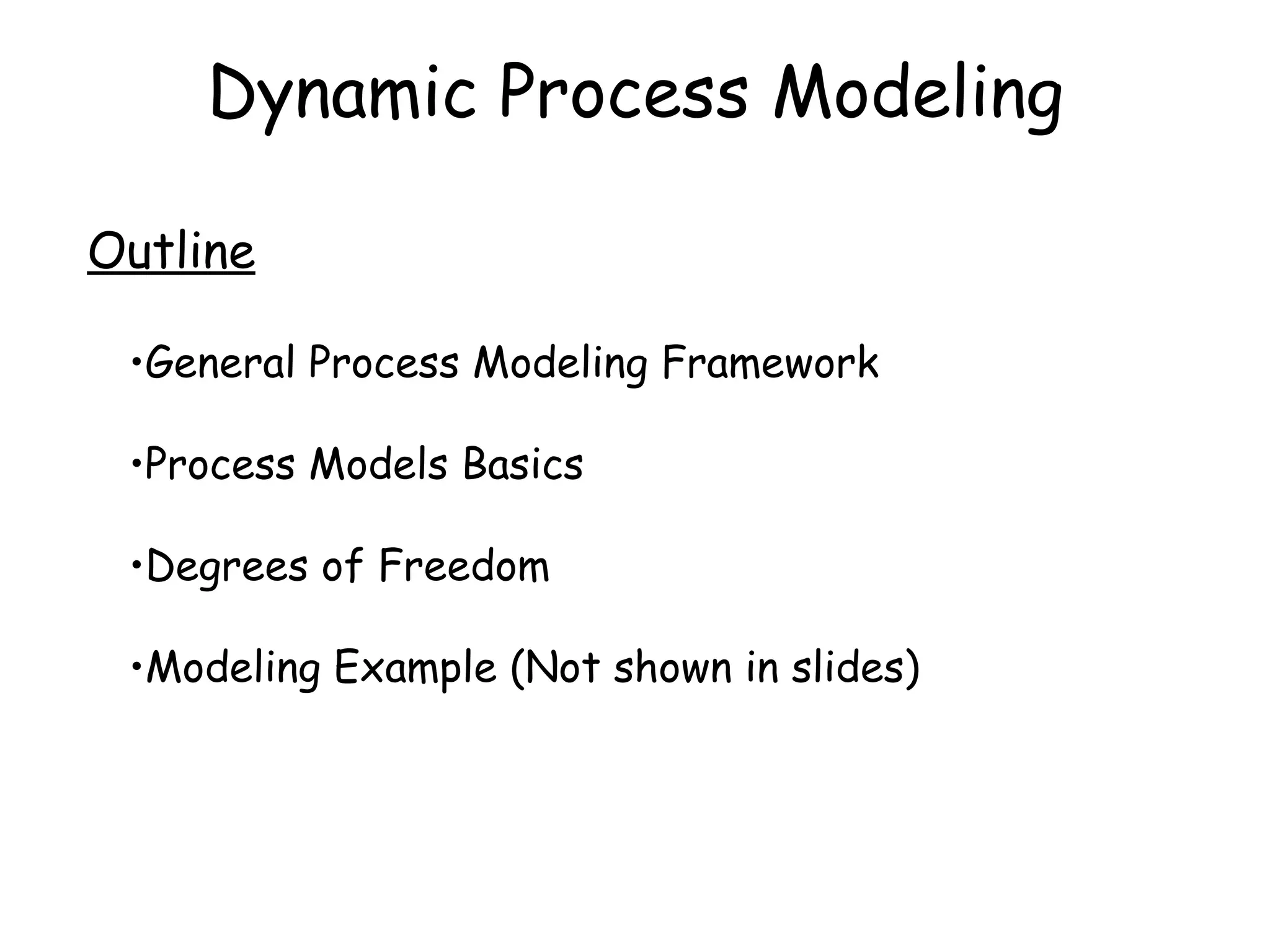
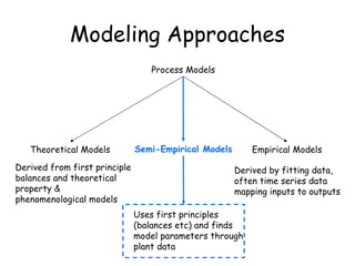
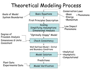
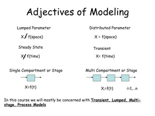
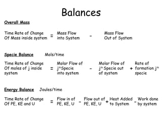
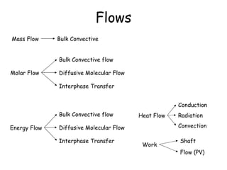
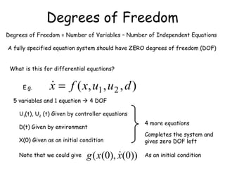
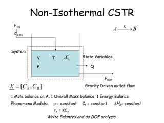
Dynamic Process Modeling

2. Modeling Approaches Theoretical Models Empirical Models Semi-Empirical Models Process Models Derived from first principle balances and theoretical property & phenomenological models Derived by fitting data, often time series data mapping inputs to outputs Uses first principles (balances etc) and finds model parameters through plant data

4. Adjectives of Modeling Lumped Parameter Distributed Parameter Steady State Transient Single Compartment or Stage Multi Compartment or Stage In this course we will mostly be concerned with Transient, Lumped, Multi-stage, Process Models X = f(space) X = f(space) X= f(time) X= f(time) X=f(t) X i =f(t) i=1,…n

5. Balances Mass Flow into System Mass Flow Out of System Time Rate of Change Of Mass inside system = - Overall Mass Molar Flow of j th Specie into system Molar Flow of j th Specie out of system Time Rate of Change Of moles of j inside system Rate of formation j th specie - = + Mols/time Specie Balance Energy Balance Time Rate of Change Of PE, KE and U Flow out of PE, KE, U Flow in of PE, KE, U Heat Added to System = Work done by system - - + Joules/time

6. Flows Mass Flow Bulk Convective Molar Flow Bulk Convective flow Interphase Transfer Diffusive Molecular Flow Energy Flow Bulk Convective flow Interphase Transfer Diffusive Molecular Flow Heat Flow Conduction Radiation Convection Work Shaft Flow (PV)

7. Molar Flows: Diffusive Diffusive Flow Molar Rate of j th specie - Diffusivity of j th specie Area Perpendicular to Transport Concentration Gradient for j A C j0 C j1  z m 2 /sec (Mol/m 3 )/m m 2 A D j = X X Diffusive Molar Flow Rate of j th specie

8. Molar Flows: Interphase If the system boundary is drown at a phase boundary then we have to consider this. Rate of Mass Transfer Mass Transfer Coefficient Interfacial Area Concentration Driving Force m/s m 2 mol/m 3 F V L F V L L

9. Heat Flows Convective from surface T Sys T A q Conduction T Sys T A L Radiation from Body T Sys Large enclosure T A Written as heat added to system

10. Reaction Terms Affect the molar & heat balances r j =reaction rate of j= K*f(C j ,…) C j = concentration of j mol/m 3 If j is a reactant then the generation term in the mole balance: -r j * V V is the volume of the vessel/compartment K has units of per time and appropriate m 3 /mol to make r j mol/m 3 /time Heat Balance -r j * V*  H R This term included (note negative sign) Note also that the reaction rate term has exponential temperature dependence

11. Degrees of Freedom Degrees of Freedom = Number of Variables – Number of Independent Equations A fully specified equation system should have ZERO degrees of freedom (DOF) What is this for differential equations? E.g. 5 variables and 1 equation  4 DOF U 1 (t), U 2 (t) Given by controller equations D(t) Given by environment X(0) Given as an initial condition 4 more equations Completes the system and gives zero DOF left Note that we could give As an initial condition

13. Non-Isothermal CSTR V T State Variables r A = KC A F IN F OUT C A,IN 1 Mole balance on A, 1 Overall Mass balance, 1 Energy Balance Phenomena Models:  = constant C P = constant Q System  H R = constant P Write Balances and do DOF analysis Gravity Driven outlet flow