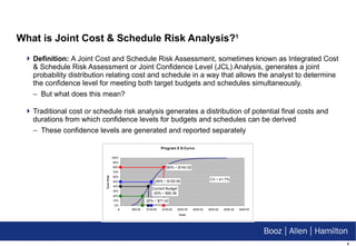
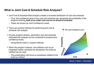
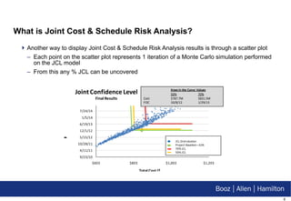
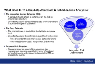
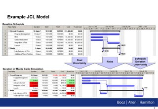
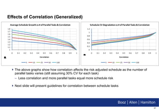
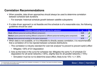
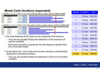
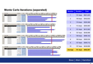
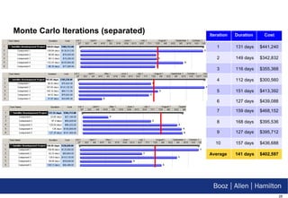
JCL in a Nutshell Demystifying the Analysis 2011 NASA PM Challenge Long Beach, CA Eric Druker This document is confidential and is intended solely for the use and information of the client to whom it is addressed. Used with permission
Abstract With agencies such as NASA now requiring joint cost and schedule risk analysis, it is important to take time out to understand the mathematics underlying both and how it relates to their integration. Rather than focusing on difficult-to-penetrate equations, this presentation will examine the math behind Joint Cost & Schedule (JCL) risk analysis using illustrative examples. These examples will demonstrate that the combination of cost & schedule risk analysis can lead to counterintuitive results. Following these demonstrations, several recommendations will be made to the community to encourage discussion and feedback regarding this emergent methodology The presentation will begin by defining joint cost & schedule risk analysis and listing several methodologies for integrating the two activities. Focusing on the Build Up method utilizing a project’s Integrated-Master Schedule; it will then lay the groundwork for the remainder of the presentation with toy problems examining how traditional cost risk analysis and schedule risk analysis (using only serial tasks) are mathematically analogous. Both the risk-adjusted cost estimate and risk-adjusted finish date represent sums of random variables and thus fall victim to the “Square Root of N Effect” where, without the injection of correlation, the Coefficient of Variation (CV) of the sum is decreased.  Unfortunately, the addition of parallel paths into the schedule dramatically complicates the analysis. No longer represented by the sum of serial tasks, the finish date is now represented by the maximum of the random variables representing the tasks in the schedule. A direct consequence of this is the fact, demonstrated previously by other papers, that increasing the symmetric uncertainty of underlying parallel tasks leads to an increase in the mean finish date. Additionally, parallel tasks fall prey to their own version of the “Square Root of N Effect.” In schedule, ignoring correlation between schedule tasks leads to an overstatement of schedule risk (increases the most likely finish date) and an understatement of the schedule CV (decreases the CV of the project’s duration). Thus, unlike in cost risk analysis where correlation only impacts the spread around the most likely cost, correlation in schedule risk analysis has a direct effect on the most likely finish date itself. Depending on how resources or costs are loaded into the schedule, this contrast between how correlation affects cost and schedule leads to the need to find a “Goldilocks” zone for correlation where it is large enough to prevent the compression of CV for cost, but not so large that it provides a false sense of security by artificially reducing the risk-adjusted finish date. The paper will conclude with recommendations for the correlation to use in JCL risk analysis.
Introduction to Joint Cost & Schedule (JCL) Risk Analysis JCL Paradoxes Typical Cost Risk Analysis Example The Merge Bias The Correlation Effect Schedule Risk Analysis Correlation Guideline Recommendations Conclusion Outline
What is Joint Cost & Schedule Risk Analysis? 1 Definition:  A Joint Cost and Schedule Risk Assessment, sometimes known as Integrated Cost & Schedule Risk Assessment or Joint Confidence Level (JCL) Analysis, generates a joint probability distribution relating cost and schedule in a way that allows the analyst to determine the confidence level for meeting both target budgets and schedules simultaneously.  But what does this mean? Traditional cost  or  schedule risk analysis generates a distribution of potential final costs and durations from which confidence levels for budgets and schedules can be derived These confidence levels are generated and reported separately
What is Joint Cost & Schedule Risk Analysis? Joint Cost & Schedule Risk Analysis creates a bivariate distribution of cost and schedule Thus, the confidence level of any cost and schedule pair represents the probability of the program finishing  both at-or-under cost and on-or-ahead of schedule These are known as Joint Confidence Levels There are several methods for performing joint cost & schedule risk analysis At early program phases, parametric cost and schedule estimates/risk analysis can be combined to produce joint confidence levels Using Monte Carlo or Copula methods When the program matures, and artifacts such as an integrated master schedule are developed, the build-up method can be used This presentation will focus on paradoxes related to the build-up method Cost Probability 70% Joint Confidence Level Schedule
What is Joint Cost & Schedule Risk Analysis? Another way to display Joint Cost & Schedule Risk Analysis results is through a scatter plot Each point on the scatter plot represents 1 iteration of a Monte Carlo simulation performed on the JCL model From this any % JCL can be uncovered
What Goes In To a Build-Up Joint Cost & Schedule Risk Analysis? The Integrated Master Schedule (IMS) A schedule health check is performed on the IMS to ensure logic structure Uncertainty around schedule tasks (at a level where there is sufficient insight) is quantified The Cost Estimate The cost estimate is loaded into the IMS at a summary level Uncertainty around the estimate is quantified; broken into: Time-Dependent Costs: Increase as Schedule Grows Time-Independent Costs: Independent of Schedule Program Risk Register Risks managed as a part of the program’s risk management plan are quantified in terms of cost and schedule impacts and mapped to tasks in the IMS as probabilistic events
Example JCL Model Cost Uncertainty Risks Schedule Duration Uncertainty Iteration of Monte Carlo Simulation Baseline Schedule
The JCL Paradoxes The buildup method seems simple enough, why dedicate a paper to it? There are two paradoxes of the build-up methodology that risk analysts and project managers need to be aware of Under most circumstances, the inclusion of parallel tasks in the schedule will cause the deterministic schedule to be at a low confidence level 2 Known as the merge bias 3 True even when symmetric uncertainty is applied Correlation between schedule duration distributions has a direct effect on both the mean and variance of the risk adjusted program completion date and must be accounted for In cost risk analysis, correlation only affects the spread of the cost distribution It is important that cost and schedule risk analysts understand both of these paradoxes as they are important to performing JCL analysis Guidelines for correlation between schedule distributions will be included
A Typical Cost Risk Analysis Assume a satellite consists of 5 components, with the cost estimate for each distributed as a normal distribution with a mean of $80K and a CV of 30% With no correlation, the total cost of the satellite has a mean of $400K and a CV of 13% Decrease of CV to 13.4% caused by “Square Root of n Effect” Cost risk analysis is fairly simple as it only deals with the summation of random variables As would schedule risk analysis be if it only dealt with serial tasks Let’s look at how schedule parallelism turns the above logic on its head
The Merge Bias: A Simple Example Suppose you and your friend are driving from separate locations to meet up for dinner and you need to decide at what time to make reservations After talking, you both decide you will leave work at 5:00 pm Each of you estimates that it will take 30 minutes to get to the restaurant (at the median) Reservations are made for 5:30 pm, what is the probability you both will make dinner on time? If each driver has a 50% probability of arriving at dinner on time then, assuming independence, the probability the party as a whole arrives on time is 25% Same as the probability of getting two heads in flips of a fair coin This example is intuitively simple, let’s return to our satellite program
The Merge Bias: A Satellite Development Program Example Satellite programs generally have several components being constructed in parallel To complete the satellite, all components must be complete In this satellite example, 5 components are being built in parallel What is the distribution of the completion date of the system? Of it’s final cost? For simplicity, let us assume the duration to build each element is normally distributed with a mean of 100 days and a standard deviation of 30 days In terms of cost, each schedule element spends at the rate of $100 per hour We’ll use a Monte Carlo simulation to perform this JCL analysis
Monte Carlo Iterations The satellite’s finish date is the  maximum  of the finish dates of the 5 components For most iterations (97%) there is one component that overruns Probability of finishing on time is 50%^5 = 3% At the same time, cost is still driven by the individual,  symmetrically distributed  component durations Thus we are actually finding the distribution of the  sum  of random variables This is analogous to traditional cost estimating The next slide will show the results of 10,000 runs of this simulation *Red line denotes baseline schedule This slide needs to be viewed in slide show mode; otherwise see backup for iterations Iteration Duration Cost 1 131 days $441,240 2 149 days $342,832 3 116 days $355,368 4 112 days $300,560 5 151 days $413,392 6 127 days $439,088 7 159 days $468,152 8 168 days $395,536 9 127 days $395,712 10 157 days $436,688 Average 141 days $402,597
Results The deterministic schedule is at 3% confidence with 34% schedule risk to the median completion date 3% confidence = (50% probability each component finishes on time)^(5 components) 34% represents 5 th  order statistic of 5 iid N(100, 30) random variables Is this really realistic? Without correlation we may be overstating risk (more on this later) Point cost estimate is at 50% confidence with 0% cost growth to the median
The Merge Bias and Order Statistics In cost risk analysis, results can be cross-checked using the central limit theorem Method of Moments can (and should) be used to cross-check mean and standard deviation In schedule risk analysis there is no simple way to mathematically check the expected finish date of a complex schedule network Serial tasks are simple; since they can be summed the math is the same as traditional cost risk analysis Parallelism introduces a significant layer of complexity as the finish date of the parallel schedule network is constrained by the maximum of finish dates Calculating the maximum of schedule distribution requires the use of order statistics Closed form equations for order statistics are very limited For example, the distribution of the k th  statistic from  iid,  continuous random variables is:
Complex Schedule Networks Unfortunately, real-world schedules have far more than just parallel tasks to deal with: Due to the complexity of large schedules, Monte Carlo analysis is the only reasonable away to evaluate schedule risk using the build-up method It is important that risk analysts effectively communicate to PMs how the topology of their schedule will affect the results Schedule parallelism, cross-links and high uncertainty factors will all cause the baseline plan to be at a low confidence level unless significant reserves and slack are in the schedule Margin should be determined based on results from risk analysis Without correlation however, this effect (the “Merge Bias”), is likely to be overstated Similarly the CV of the cost distribution will be understated To examine how correlation affects schedules, let’s return to our dinner example Factors Influencing Schedule Risk Mix of Parallel/Serial Tasks Types of Task Constraints (Start no Earlier Than, Must Start On, etc.) Resource Availabilities Types of Task Relationships (Start to Start, Start to Finish, Finish to Finish, etc) Cross-links/dependencies Schedule Margin, Schedule Slack, Schedule Reserves
Correlation (cite CEBoK) Although the two parties are driving separately, there are factors likely to affect both: Traffic, difficulties in finding parking spaces and weather will affect both drivers similarly Similarly, each driver has factors that are independent The risk of breaking down or getting in an accident will be independent between drivers Since there are similarities and differences between the drives, it is impossible to argue that travel times to dinner are uncorrelated or perfectly correlated Rather, they must be somewhere in between Driver 1 Travel Time Driver 2 Travel Time No Correlation Driver 1 Travel Time Driver 2 Travel Time Some Correlation Driver 1 Travel Time Driver 2 Travel Time Perfect Correlation
Correlation: A Simple Example In the dinner example, with zero correlation, the probability of both parties arriving on time was 25% As correlation rises, the probability of both parties arriving on time increases This is because extreme disparities (one driver arriving very early, one very late) are reduced Similarly, the CV of the arrival time increases R 2  = 0 R 2  = 0.25 R 2  = 1 Green box denotes both parties arriving on time for dinner Assumptions 5000 Monte Carlo Runs. Commute times distributed as N(30 minutes, 9 minutes) ρ  of 1 = Parties Take Same Car
Today’s Schedule Risk Analysis Standards Many schedule risk analysts ignore correlation between schedule tasks using the rationale that “it’s covered in the schedule logic” The correlation inferred by that statement only addresses schedule slips I.e. If development takes longer, integration will be  delayed Injecting correlation between schedule task duration distributions accounts for this omission I.e. If development takes longer, integration will be delayed  and is likely to take longer This is because difficulties (or, conversely, successes) in overcoming the problem or schedule underestimations are likely to be systemic to a program Omitting correlation leads to an overstatement of schedule risk Also an underestimation of cost and schedule uncertainty No Cost or Schedule Risk Analysis is Valid If It Has Not Addressed Correlation
Effects of Correlation on Satellite Example Above graph represents effects of injecting correlation between component durations from the spacecraft example As correlation increases, CV of both cost and schedule distributions increases and expected finish date of the schedule improves If there are similar factors affecting schedule tasks it is practically inconceivable that they could be uncorrelated Next slide will examine schedule risk as the number of parallel tasks varies 5 Parallel Tasks ~ N(100, 30) With a correlation of  .3 (blue line)  between schedule tasks: CV of the schedule duration distribution is 18% (or  60%  of the input task duration CVs of 30%) CV of the cost distribution is 19% (or  65%  of the input task duration CVs of 30%) The average schedule duration is 129 days (or 129% of the baseline schedule duration of 100 days) Graph Explanation
Effects of Correlation (Generalized) The above graphs show how correlation affects the risk adjusted schedule as the number of parallel tasks varies (still assuming 30% CV for each task) Less correlation and more parallel tasks equal more schedule risk Next slide will present guidelines for correlation between schedule tasks
Correlation Recommendations When possible, data driven approaches should always be used to determine correlation between schedule task durations For example: historical schedule growth between satellite subsystems If a data driven approach is not feasible and the schedule is of a reasonable size, the following guidelines should be used When data is not available, or it is infeasible to directly assess correlation, it is recommended that a correlation of 0.3 be injected between schedule distributions This correlation is industry standard for cost risk analysis 4  to prevent to prevent sqrt(n) effect Mitigates ~30% of CV degradation Acts as the knee in the curve for schedule risk: Mitigates the same % of schedule CV degradation for all serial networks (~30%), slightly less for all parallel networks (~15%) Simulation must be run to determine exact effect, likely to be 15% < x < 30% *It is extraordinarily rare for tasks on the same project to be completely uncorrelated ( ρ  = 0). Similarly, if two tasks are perfectly correlated ( ρ  = 1) they should be functionally linked Correlation (including example basis for selection)* ρ Pic Weak  (different personnel working different component) 0.25 Medium  (same personnel working different component or different personnel working same component) 0.50 Strong  (same personnel working on the same component) 0.75
Conclusion & Recommendations As a community, risk analysts need to understand, and be able to communicate, the two JCL Paradoxes Schedule parallelism, a high number of cross-links between activities and large uncertainties on task durations will lead to a high risk adjusted finish date … and low confidence in the deterministic schedule Correlation is a significant driver of schedule risk and must be accounted for in all schedule risk analysis Ignoring correlation leads to an overstatement of schedule risk and an underestimation of both the cost and schedule CVs It is hoped that the correlation guidelines provided in this presentation can begin the conversation regarding how correlation should be handled in both JCL and schedule risk analysis
Works Cited 1  Druker, Eric. “Emerging Practice: Joint Cost & Schedule Risk Analysis.” 2009 Institute for Operations Research and the Management Sciences Annual Meeting. San Diego, CA. October 2009 2  Coleman, Richard. Summerville, Jessica. “The Relationship Between Cost Growth and Schedule Growth.”  Acquisition Review Quarterly.  Spring 2003 3  Hulett, David.  Practical Schedule Risk Analysis . Burlington: Gower Publishing Company, 2009. 4  Book, Stephen. “Why Correlation Matters in Cost Estimating.” 32 nd  Annual Department of Defense Cost Analysis Symposium. Williamsburg, VA. February 1999.
Backup Filename/RPS Number
Monte Carlo Iterations (separated) For most iterations (97%) there is one component that overruns Thus we are actually finding the distribution of the  maximum  of random variables Even with symmetric uncertainty, this will always be greater than the critical path length At the same time, cost is still driven by the individual,  symmetrically distributed  component durations Thus we are actually finding the distribution of the  sum  of random variables Iteration Duration Cost 1 131 days $441,240 2 149 days $342,832 3 116 days $355,368 4 112 days $300,560 5 151 days $413,392 6 127 days $439,088 7 159 days $468,152 8 168 days $395,536 9 127 days $395,712 10 157 days $436,688 Average 141 days $402,597
Monte Carlo Iterations (separated) Iteration Duration Cost 1 131 days $441,240 2 149 days $342,832 3 116 days $355,368 4 112 days $300,560 5 151 days $413,392 6 127 days $439,088 7 159 days $468,152 8 168 days $395,536 9 127 days $395,712 10 157 days $436,688 Average 141 days $402,597

Druker

  • 1.
    JCL in aNutshell Demystifying the Analysis 2011 NASA PM Challenge Long Beach, CA Eric Druker This document is confidential and is intended solely for the use and information of the client to whom it is addressed. Used with permission
  • 2.
    Abstract With agenciessuch as NASA now requiring joint cost and schedule risk analysis, it is important to take time out to understand the mathematics underlying both and how it relates to their integration. Rather than focusing on difficult-to-penetrate equations, this presentation will examine the math behind Joint Cost & Schedule (JCL) risk analysis using illustrative examples. These examples will demonstrate that the combination of cost & schedule risk analysis can lead to counterintuitive results. Following these demonstrations, several recommendations will be made to the community to encourage discussion and feedback regarding this emergent methodology The presentation will begin by defining joint cost & schedule risk analysis and listing several methodologies for integrating the two activities. Focusing on the Build Up method utilizing a project’s Integrated-Master Schedule; it will then lay the groundwork for the remainder of the presentation with toy problems examining how traditional cost risk analysis and schedule risk analysis (using only serial tasks) are mathematically analogous. Both the risk-adjusted cost estimate and risk-adjusted finish date represent sums of random variables and thus fall victim to the “Square Root of N Effect” where, without the injection of correlation, the Coefficient of Variation (CV) of the sum is decreased. Unfortunately, the addition of parallel paths into the schedule dramatically complicates the analysis. No longer represented by the sum of serial tasks, the finish date is now represented by the maximum of the random variables representing the tasks in the schedule. A direct consequence of this is the fact, demonstrated previously by other papers, that increasing the symmetric uncertainty of underlying parallel tasks leads to an increase in the mean finish date. Additionally, parallel tasks fall prey to their own version of the “Square Root of N Effect.” In schedule, ignoring correlation between schedule tasks leads to an overstatement of schedule risk (increases the most likely finish date) and an understatement of the schedule CV (decreases the CV of the project’s duration). Thus, unlike in cost risk analysis where correlation only impacts the spread around the most likely cost, correlation in schedule risk analysis has a direct effect on the most likely finish date itself. Depending on how resources or costs are loaded into the schedule, this contrast between how correlation affects cost and schedule leads to the need to find a “Goldilocks” zone for correlation where it is large enough to prevent the compression of CV for cost, but not so large that it provides a false sense of security by artificially reducing the risk-adjusted finish date. The paper will conclude with recommendations for the correlation to use in JCL risk analysis.
  • 3.
    Introduction to JointCost & Schedule (JCL) Risk Analysis JCL Paradoxes Typical Cost Risk Analysis Example The Merge Bias The Correlation Effect Schedule Risk Analysis Correlation Guideline Recommendations Conclusion Outline
  • 4.
    What is JointCost & Schedule Risk Analysis? 1 Definition: A Joint Cost and Schedule Risk Assessment, sometimes known as Integrated Cost & Schedule Risk Assessment or Joint Confidence Level (JCL) Analysis, generates a joint probability distribution relating cost and schedule in a way that allows the analyst to determine the confidence level for meeting both target budgets and schedules simultaneously. But what does this mean? Traditional cost or schedule risk analysis generates a distribution of potential final costs and durations from which confidence levels for budgets and schedules can be derived These confidence levels are generated and reported separately
  • 5.
    What is JointCost & Schedule Risk Analysis? Joint Cost & Schedule Risk Analysis creates a bivariate distribution of cost and schedule Thus, the confidence level of any cost and schedule pair represents the probability of the program finishing both at-or-under cost and on-or-ahead of schedule These are known as Joint Confidence Levels There are several methods for performing joint cost & schedule risk analysis At early program phases, parametric cost and schedule estimates/risk analysis can be combined to produce joint confidence levels Using Monte Carlo or Copula methods When the program matures, and artifacts such as an integrated master schedule are developed, the build-up method can be used This presentation will focus on paradoxes related to the build-up method Cost Probability 70% Joint Confidence Level Schedule
  • 6.
    What is JointCost & Schedule Risk Analysis? Another way to display Joint Cost & Schedule Risk Analysis results is through a scatter plot Each point on the scatter plot represents 1 iteration of a Monte Carlo simulation performed on the JCL model From this any % JCL can be uncovered
  • 7.
    What Goes InTo a Build-Up Joint Cost & Schedule Risk Analysis? The Integrated Master Schedule (IMS) A schedule health check is performed on the IMS to ensure logic structure Uncertainty around schedule tasks (at a level where there is sufficient insight) is quantified The Cost Estimate The cost estimate is loaded into the IMS at a summary level Uncertainty around the estimate is quantified; broken into: Time-Dependent Costs: Increase as Schedule Grows Time-Independent Costs: Independent of Schedule Program Risk Register Risks managed as a part of the program’s risk management plan are quantified in terms of cost and schedule impacts and mapped to tasks in the IMS as probabilistic events
  • 8.
    Example JCL ModelCost Uncertainty Risks Schedule Duration Uncertainty Iteration of Monte Carlo Simulation Baseline Schedule
  • 9.
    The JCL ParadoxesThe buildup method seems simple enough, why dedicate a paper to it? There are two paradoxes of the build-up methodology that risk analysts and project managers need to be aware of Under most circumstances, the inclusion of parallel tasks in the schedule will cause the deterministic schedule to be at a low confidence level 2 Known as the merge bias 3 True even when symmetric uncertainty is applied Correlation between schedule duration distributions has a direct effect on both the mean and variance of the risk adjusted program completion date and must be accounted for In cost risk analysis, correlation only affects the spread of the cost distribution It is important that cost and schedule risk analysts understand both of these paradoxes as they are important to performing JCL analysis Guidelines for correlation between schedule distributions will be included
  • 10.
    A Typical CostRisk Analysis Assume a satellite consists of 5 components, with the cost estimate for each distributed as a normal distribution with a mean of $80K and a CV of 30% With no correlation, the total cost of the satellite has a mean of $400K and a CV of 13% Decrease of CV to 13.4% caused by “Square Root of n Effect” Cost risk analysis is fairly simple as it only deals with the summation of random variables As would schedule risk analysis be if it only dealt with serial tasks Let’s look at how schedule parallelism turns the above logic on its head
  • 11.
    The Merge Bias:A Simple Example Suppose you and your friend are driving from separate locations to meet up for dinner and you need to decide at what time to make reservations After talking, you both decide you will leave work at 5:00 pm Each of you estimates that it will take 30 minutes to get to the restaurant (at the median) Reservations are made for 5:30 pm, what is the probability you both will make dinner on time? If each driver has a 50% probability of arriving at dinner on time then, assuming independence, the probability the party as a whole arrives on time is 25% Same as the probability of getting two heads in flips of a fair coin This example is intuitively simple, let’s return to our satellite program
  • 12.
    The Merge Bias:A Satellite Development Program Example Satellite programs generally have several components being constructed in parallel To complete the satellite, all components must be complete In this satellite example, 5 components are being built in parallel What is the distribution of the completion date of the system? Of it’s final cost? For simplicity, let us assume the duration to build each element is normally distributed with a mean of 100 days and a standard deviation of 30 days In terms of cost, each schedule element spends at the rate of $100 per hour We’ll use a Monte Carlo simulation to perform this JCL analysis
  • 13.
    Monte Carlo IterationsThe satellite’s finish date is the maximum of the finish dates of the 5 components For most iterations (97%) there is one component that overruns Probability of finishing on time is 50%^5 = 3% At the same time, cost is still driven by the individual, symmetrically distributed component durations Thus we are actually finding the distribution of the sum of random variables This is analogous to traditional cost estimating The next slide will show the results of 10,000 runs of this simulation *Red line denotes baseline schedule This slide needs to be viewed in slide show mode; otherwise see backup for iterations Iteration Duration Cost 1 131 days $441,240 2 149 days $342,832 3 116 days $355,368 4 112 days $300,560 5 151 days $413,392 6 127 days $439,088 7 159 days $468,152 8 168 days $395,536 9 127 days $395,712 10 157 days $436,688 Average 141 days $402,597
  • 14.
    Results The deterministicschedule is at 3% confidence with 34% schedule risk to the median completion date 3% confidence = (50% probability each component finishes on time)^(5 components) 34% represents 5 th order statistic of 5 iid N(100, 30) random variables Is this really realistic? Without correlation we may be overstating risk (more on this later) Point cost estimate is at 50% confidence with 0% cost growth to the median
  • 15.
    The Merge Biasand Order Statistics In cost risk analysis, results can be cross-checked using the central limit theorem Method of Moments can (and should) be used to cross-check mean and standard deviation In schedule risk analysis there is no simple way to mathematically check the expected finish date of a complex schedule network Serial tasks are simple; since they can be summed the math is the same as traditional cost risk analysis Parallelism introduces a significant layer of complexity as the finish date of the parallel schedule network is constrained by the maximum of finish dates Calculating the maximum of schedule distribution requires the use of order statistics Closed form equations for order statistics are very limited For example, the distribution of the k th statistic from iid, continuous random variables is:
  • 16.
    Complex Schedule NetworksUnfortunately, real-world schedules have far more than just parallel tasks to deal with: Due to the complexity of large schedules, Monte Carlo analysis is the only reasonable away to evaluate schedule risk using the build-up method It is important that risk analysts effectively communicate to PMs how the topology of their schedule will affect the results Schedule parallelism, cross-links and high uncertainty factors will all cause the baseline plan to be at a low confidence level unless significant reserves and slack are in the schedule Margin should be determined based on results from risk analysis Without correlation however, this effect (the “Merge Bias”), is likely to be overstated Similarly the CV of the cost distribution will be understated To examine how correlation affects schedules, let’s return to our dinner example Factors Influencing Schedule Risk Mix of Parallel/Serial Tasks Types of Task Constraints (Start no Earlier Than, Must Start On, etc.) Resource Availabilities Types of Task Relationships (Start to Start, Start to Finish, Finish to Finish, etc) Cross-links/dependencies Schedule Margin, Schedule Slack, Schedule Reserves
  • 17.
    Correlation (cite CEBoK)Although the two parties are driving separately, there are factors likely to affect both: Traffic, difficulties in finding parking spaces and weather will affect both drivers similarly Similarly, each driver has factors that are independent The risk of breaking down or getting in an accident will be independent between drivers Since there are similarities and differences between the drives, it is impossible to argue that travel times to dinner are uncorrelated or perfectly correlated Rather, they must be somewhere in between Driver 1 Travel Time Driver 2 Travel Time No Correlation Driver 1 Travel Time Driver 2 Travel Time Some Correlation Driver 1 Travel Time Driver 2 Travel Time Perfect Correlation
  • 18.
    Correlation: A SimpleExample In the dinner example, with zero correlation, the probability of both parties arriving on time was 25% As correlation rises, the probability of both parties arriving on time increases This is because extreme disparities (one driver arriving very early, one very late) are reduced Similarly, the CV of the arrival time increases R 2 = 0 R 2 = 0.25 R 2 = 1 Green box denotes both parties arriving on time for dinner Assumptions 5000 Monte Carlo Runs. Commute times distributed as N(30 minutes, 9 minutes) ρ of 1 = Parties Take Same Car
  • 19.
    Today’s Schedule RiskAnalysis Standards Many schedule risk analysts ignore correlation between schedule tasks using the rationale that “it’s covered in the schedule logic” The correlation inferred by that statement only addresses schedule slips I.e. If development takes longer, integration will be delayed Injecting correlation between schedule task duration distributions accounts for this omission I.e. If development takes longer, integration will be delayed and is likely to take longer This is because difficulties (or, conversely, successes) in overcoming the problem or schedule underestimations are likely to be systemic to a program Omitting correlation leads to an overstatement of schedule risk Also an underestimation of cost and schedule uncertainty No Cost or Schedule Risk Analysis is Valid If It Has Not Addressed Correlation
  • 20.
    Effects of Correlationon Satellite Example Above graph represents effects of injecting correlation between component durations from the spacecraft example As correlation increases, CV of both cost and schedule distributions increases and expected finish date of the schedule improves If there are similar factors affecting schedule tasks it is practically inconceivable that they could be uncorrelated Next slide will examine schedule risk as the number of parallel tasks varies 5 Parallel Tasks ~ N(100, 30) With a correlation of .3 (blue line) between schedule tasks: CV of the schedule duration distribution is 18% (or 60% of the input task duration CVs of 30%) CV of the cost distribution is 19% (or 65% of the input task duration CVs of 30%) The average schedule duration is 129 days (or 129% of the baseline schedule duration of 100 days) Graph Explanation
  • 21.
    Effects of Correlation(Generalized) The above graphs show how correlation affects the risk adjusted schedule as the number of parallel tasks varies (still assuming 30% CV for each task) Less correlation and more parallel tasks equal more schedule risk Next slide will present guidelines for correlation between schedule tasks
  • 22.
    Correlation Recommendations Whenpossible, data driven approaches should always be used to determine correlation between schedule task durations For example: historical schedule growth between satellite subsystems If a data driven approach is not feasible and the schedule is of a reasonable size, the following guidelines should be used When data is not available, or it is infeasible to directly assess correlation, it is recommended that a correlation of 0.3 be injected between schedule distributions This correlation is industry standard for cost risk analysis 4 to prevent to prevent sqrt(n) effect Mitigates ~30% of CV degradation Acts as the knee in the curve for schedule risk: Mitigates the same % of schedule CV degradation for all serial networks (~30%), slightly less for all parallel networks (~15%) Simulation must be run to determine exact effect, likely to be 15% < x < 30% *It is extraordinarily rare for tasks on the same project to be completely uncorrelated ( ρ = 0). Similarly, if two tasks are perfectly correlated ( ρ = 1) they should be functionally linked Correlation (including example basis for selection)* ρ Pic Weak (different personnel working different component) 0.25 Medium (same personnel working different component or different personnel working same component) 0.50 Strong (same personnel working on the same component) 0.75
  • 23.
    Conclusion & RecommendationsAs a community, risk analysts need to understand, and be able to communicate, the two JCL Paradoxes Schedule parallelism, a high number of cross-links between activities and large uncertainties on task durations will lead to a high risk adjusted finish date … and low confidence in the deterministic schedule Correlation is a significant driver of schedule risk and must be accounted for in all schedule risk analysis Ignoring correlation leads to an overstatement of schedule risk and an underestimation of both the cost and schedule CVs It is hoped that the correlation guidelines provided in this presentation can begin the conversation regarding how correlation should be handled in both JCL and schedule risk analysis
  • 24.
    Works Cited 1 Druker, Eric. “Emerging Practice: Joint Cost & Schedule Risk Analysis.” 2009 Institute for Operations Research and the Management Sciences Annual Meeting. San Diego, CA. October 2009 2 Coleman, Richard. Summerville, Jessica. “The Relationship Between Cost Growth and Schedule Growth.” Acquisition Review Quarterly. Spring 2003 3 Hulett, David. Practical Schedule Risk Analysis . Burlington: Gower Publishing Company, 2009. 4 Book, Stephen. “Why Correlation Matters in Cost Estimating.” 32 nd Annual Department of Defense Cost Analysis Symposium. Williamsburg, VA. February 1999.
  • 25.
  • 26.
    Monte Carlo Iterations(separated) For most iterations (97%) there is one component that overruns Thus we are actually finding the distribution of the maximum of random variables Even with symmetric uncertainty, this will always be greater than the critical path length At the same time, cost is still driven by the individual, symmetrically distributed component durations Thus we are actually finding the distribution of the sum of random variables Iteration Duration Cost 1 131 days $441,240 2 149 days $342,832 3 116 days $355,368 4 112 days $300,560 5 151 days $413,392 6 127 days $439,088 7 159 days $468,152 8 168 days $395,536 9 127 days $395,712 10 157 days $436,688 Average 141 days $402,597
  • 27.
    Monte Carlo Iterations(separated) Iteration Duration Cost 1 131 days $441,240 2 149 days $342,832 3 116 days $355,368 4 112 days $300,560 5 151 days $413,392 6 127 days $439,088 7 159 days $468,152 8 168 days $395,536 9 127 days $395,712 10 157 days $436,688 Average 141 days $402,597
  • 28.
    Monte Carlo Iterations(separated) Iteration Duration Cost 1 131 days $441,240 2 149 days $342,832 3 116 days $355,368 4 112 days $300,560 5 151 days $413,392 6 127 days $439,088 7 159 days $468,152 8 168 days $395,536 9 127 days $395,712 10 157 days $436,688 Average 141 days $402,597