Advanced Project Schedule Risk Analysis-13th Annual International Integrated program management.pdf

1. 1
Advanced Project
Schedule Risk Analysis
13th Annual International
Integrated Program Management
David T. Hulett, Ph.D.
Hulett & Associates, LLC
Project Management Consultants
Los Angeles, CA
(310) 476-7699
info@projectrisk.com
© 2001 Hulett & Associates, LLC

2. 2
Agenda
• Uncertain activity durations
• Simple one-path schedule risk
• Risk at merge points: the “Merge Bias”
• Correlation among uncertain durations
• Probabilistic Branching
• Conditional Branching
• Resources
• Constraints

3. 3
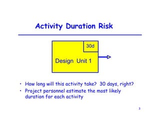
Activity Duration Risk
• How long will this activity take? 30 days, right?
• Project personnel estimate the most likely
duration for each activity
Design Unit 1
30d

4. 4
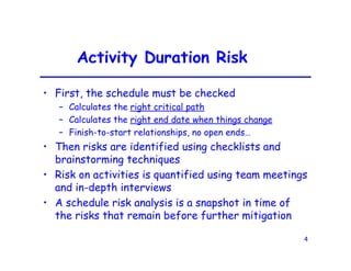
Activity Duration Risk
• First, the schedule must be checked
– Calculates the right critical path
– Calculates the right end date when things change
– Finish-to-start relationships, no open ends…
• Then risks are identified using checklists and
brainstorming techniques
• Risk on activities is quantified using team meetings
and in-depth interviews
• A schedule risk analysis is a snapshot in time of
the risks that remain before further mitigation

5. 5
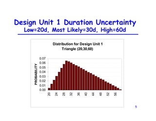
Design Unit 1 Duration Uncertainty
Low=20d, Most Likely=30d, High=60d
Distribution for Design Unit 1
Triangle (20,30,60)
0.00
0.01
0.02
0.03
0.04
0.05
0.06
0.07
20
24
28
32
36
40
44
48
52
56
PROBABILITY

6. 6
Risk Along a Path
Start Design Unit 1 Build Unit 1 Finish

7. 7
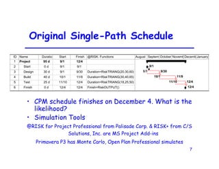
Original Single-Path Schedule
• CPM schedule finishes on December 4. What is the
likelihood?
• Simulation Tools
@RISK for Project Professional from Palisade Corp. & RISK+ from C/S
Solutions, Inc. are MS Project Add-ins
Primavera P3 has Monte Carlo, Open Plan Professional simulates
ID Name Duratio Start Finish @RISK: Functions
1 Project 95 d 9/1 12/4
2 Start 0 d 9/1 9/1
3 Design 30 d 9/1 9/30 Duration=RiskTRIANG(20,30,60)
4 Build 40 d 10/1 11/9 Duration=RiskTRIANG(30,40,65)
5 Test 25 d 11/10 12/4 Duration=RiskTRIANG(18,25,50)
6 Finish 0 d 12/4 12/4 Finish=RiskOUTPUT()
9/1
9/1 9/30
10/1 11/9
11/10 12/4
12/4
August Septemb
October NovembDecemb January

8. 8
Monte Carlo Simulation
• A simulation explores all combinations of durations
of uncertain (and certain) activities
• Durations are chosen at random from input
distributions
• The project is calculated (Press [F-9])
• Completion dates computed many times
• Distribution of completion dates
• Cumulative likelihood provides results

9. 9
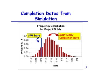
Completion Dates from
Simulation
Frequency Distribution
for Project Finish
0.00
0.02
0.04
0.06
0.08
0.10
11/15
11/24
12/3
12/12
12/21
12/30
1/8
1/17
1/26
2/4
Date
PROBABILITY
CPM Date Most Likely
Completion Date

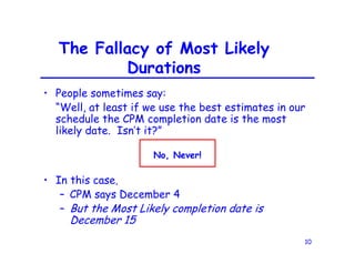
10. 10
The Fallacy of Most Likely
Durations
• People sometimes say:
“Well, at least if we use the best estimates in our
schedule the CPM completion date is the most
likely date. Isn’t it?”
No, Never!
• In this case,
– CPM says December 4
– But the Most Likely completion date is
December 15

11. 11
Cumulative Distribution --
December 10 is only 10% Likely
Cumulative Distribution
for Project Finish
0.0
0.1
0.2
0.3
0.4
0.5
0.6
0.7
0.8
0.9
1.0
11/15
11/24
12/3
12/12
12/21
12/30
1/8
1/17
1/26
2/4
Date
Prob
of
Value
<=
X-axis
Value
CPM
Date
12/4
80% Likely
Schedule 1/3

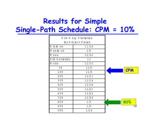
12. 12
Results for Simple
Single-Path Schedule: CPM = 10%
80%
CPM
M i
ni
m um 11/18
M axi
m um 2/6
M ean 12/22
S td D evi
ati
on 13
M ode 12/15
5% 12/1
10% 12/5
20% 12/11
30% 12/14
40% 12/18
50% 12/21
60% 12/25
70% 12/29
80% 1/3
90% 1/9
95% 1/14
S um m ary S tati
sti
cs
f
or P roj
ect F i
ni
sh

13. 13
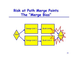
Risk at Path Merge Points
The “Merge Bias”
Start
Design Unit 1
Design Unit 2
Finish
Build Unit 1
Build Unit 2

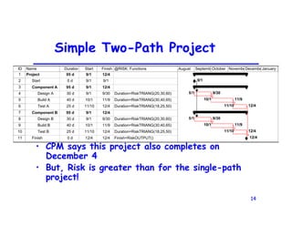
14. 14
Simple Two-Path Project
• CPM says this project also completes on
December 4
• But, Risk is greater than for the single-path
project!
ID Name Duration Start Finish @RISK: Functions
1 Project 95 d 9/1 12/4
2 Start 0 d 9/1 9/1
3 Component A 95 d 9/1 12/4
4 Design A 30 d 9/1 9/30 Duration=RiskTRIANG(20,30,60)
5 Build A 40 d 10/1 11/9 Duration=RiskTRIANG(30,40,65)
6 Test A 25 d 11/10 12/4 Duration=RiskTRIANG(18,25,50)
7 Component B 95 d 9/1 12/4
8 Design B 30 d 9/1 9/30 Duration=RiskTRIANG(20,30,60)
9 Build B 40 d 10/1 11/9 Duration=RiskTRIANG(30,40,65)
10 Test B 25 d 11/10 12/4 Duration=RiskTRIANG(18,25,50)
11 Finish 0 d 12/4 12/4 Finish=RiskOUTPUT()
9/1
9/1 9/30
10/1 11/9
11/10 12/4
9/1 9/30
10/1 11/9
11/10 12/4
12/4
August Septemb October NovembeDecembeJanuary

15. 15
Effect of the Merge Bias
D istribution forP rojectF inish
O ne and Tw o P ath S chedules
0.0
0.1
0.2
0.3
0.4
0.5
0.6
0.7
0.8
0.9
1.0
11/1
11/8
11/15
11/22
11/29
12/6
12/13
12/20
12/27
1/3
1/10
1/17
1/24
1/31
2/7
D ate
P
rob
of
value
<
=
X
-A
xis
V
alue
One-Path
Schedule
Two-Path
Schedule
CPM Date

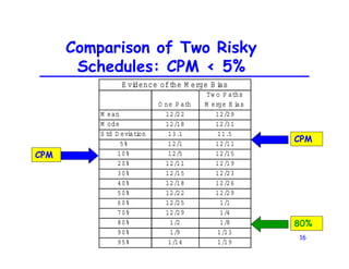
16. 16
Comparison of Two Risky
Schedules: CPM < 5%
O ne P ath
Tw o P aths
M erge B i
as
M ean 12/22 12/29
M ode 12/18 12/31
S td D evi
ati
on 13.1 11.5
5% 12/1 12/11
10% 12/5 12/15
20% 12/11 12/19
30% 12/15 12/23
40% 12/18 12/26
50% 12/22 12/29
60% 12/25 1/1
70% 12/29 1/4
80% 1/2 1/8
90% 1/9 1/13
95% 1/14 1/19
E vi
dence ofthe M erge B i
as
80%
CPM
CPM

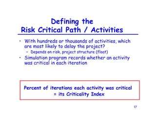
17. 17
Defining the
Risk Critical Path / Activities
• With hundreds or thousands of activities, which
are most likely to delay the project?
– Depends on risk, project structure (float)
• Simulation program records whether an activity
was critical in each iteration
Percent of iterations each activity was critical
= its Criticality Index

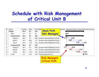
18. 18
Schedule with Risk Management
of Critical Unit B
ID Name Duration Start Finish @RISK: Functions
1 Project 95 d 9/1 12/4
2 Start 0 d 9/1 9/1
3 Component A 93 d 9/1 12/2
4 Design A 28 d 9/1 9/28 Duration=RiskTRIANG(18,28,58)
5 Build A 40 d 9/29 11/7 Duration=RiskTRIANG(30,40,65)
6 Test A 25 d 11/8 12/2 Duration=RiskTRIANG(18,25,50)
7 Component B 95 d 9/1 12/4
8 Design B 30 d 9/1 9/30 Duration=RiskTRIANG(25,30,40)
9 Build B 40 d 10/1 11/9 Duration=RiskTRIANG(35,40,50)
10 Test B 25 d 11/10 12/4 Duration=RiskTRIANG(20,25,30)
11 Finish 0 d 12/4 12/4 Finish=RiskOUTPUT()
9/1
9/1 9/28
9/29 11/7
11/8 12/2
9/1 9/30
10/1 11/9
11/10 12/4
12/4
August SeptembOctober Novemb DecembeJanuary
Slack Path
Not Managed
Risk Managed
Critical Path

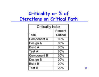
19. 19
Criticality or % of
Iterations on Critical Path
Task
Percent
Critical
Component A 80%
Design A 80%
Build A 80%
Test A 80%
Component B 20%
Design B 20%
Build B 20%
Test B 20%
Criticality Index

20. 20
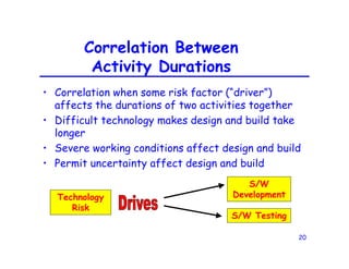
Correlation Between
Activity Durations
• Correlation when some risk factor (“driver”)
affects the durations of two activities together
• Difficult technology makes design and build take
longer
• Severe working conditions affect design and build
• Permit uncertainty affect design and build
Technology
Risk
S/W
Development
S/W Testing

21. 21
Correlation
• Correlation makes the durations “move” together
• If one activity takes longer than estimated the
other does too
• Both activities will take more (or less) time
together
• Correlation increases the risk of extreme results

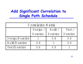
22. 22
Add Significant Correlation to
Single Path Schedule
D esign /
D uration
B uild /
D uration
Test /
D uration
D esign/D uration 1 0.8 0.6
B uild/D uration 0.8 1 0.9
Test/D uration 0.6 0.9 1
C orrel
ati
on M atri
x

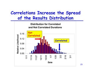
23. 23
Correlations Increase the Spread
of the Results Distribution
Distribution for Correlated
and Not Correlated Durations
0.00
0.04
0.08
0.12
0.16
11/1
11/14
11/27
12/11
12/24
1/7
1/20
2/2
2/16
3/1
Date
Relative
Likelihood
Not
Correlated
Correlated

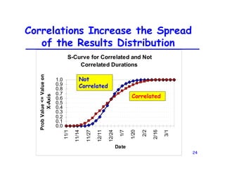
24. 24
Correlations Increase the Spread
of the Results Distribution
S-Curve for Correlated and Not
Correlated Durations
0.0
0.1
0.2
0.3
0.4
0.5
0.6
0.7
0.8
0.9
1.0
11/1
11/14
11/27
12/11
12/24
1/7
1/20
2/2
2/16
3/1
Date
Prob
Value
<=
Value
on
X-Axis
Not
Correlated
Correlated

25. 25
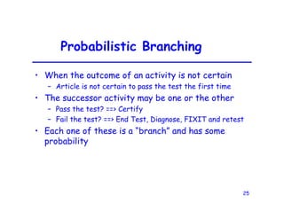
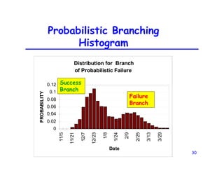
Probabilistic Branching
• When the outcome of an activity is not certain
– Article is not certain to pass the test the first time
• The successor activity may be one or the other
– Pass the test? ==> Certify
– Fail the test? ==> End Test, Diagnose, FIXIT and retest
• Each one of these is a “branch” and has some
probability

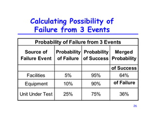
26. 26
Calculating Possibility of
Failure from 3 Events
Source of
Failure Event
Probability
of Failure
Probability
of Success
Merged
Probability
of Success
Facilities 5% 95% 64%
Equipment 10% 90% of Failure
Unit Under Test 25% 75% 36%
Probability of Failure from 3 Events

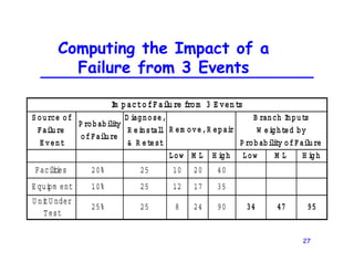
27. 27
Computing the Impact of a
Failure from 3 Events
S ource of
Failure
E vent
P robability
ofFailure
D iagnose,
R einstall
& R etest
Low M L H igh Low M L H igh
Faci
l
i
ti
es 20% 25 10 20 40
E qui
pm ent 10% 25 12 17 35
U ni
tU nder
Test
25% 25 8 24 90 34 47 95
Im pactofFai
lure from 3 E vents
R em ove,R epair
B ranch Inputs
W eighted by
P robability ofFailure

28. 28
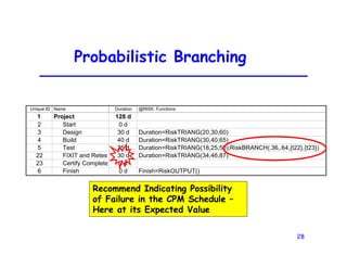
Probabilistic Branching
Unique ID Name Duration @RISK: Functions
1 Project 128 d
2 Start 0 d
3 Design 30 d Duration=RiskTRIANG(20,30,60)
4 Build 40 d Duration=RiskTRIANG(30,40,65)
5 Test 25 d Duration=RiskTRIANG(18,25,50);RiskBRANCH(.36,.64,{t22},{t23})
22 FIXIT and Retest 30 d Duration=RiskTRIANG(34,46,87)
23 Certify Complete 3 d
6 Finish 0 d Finish=RiskOUTPUT()
Recommend Indicating Possibility
of Failure in the CPM Schedule –
Here at its Expected Value

29. 29
Network Logic of Test Failure
Probabilistic Branch

30. 30
Probabilistic Branching
Histogram
Distribution for Branch
of Probabilistic Failure
0
0.02
0.04
0.06
0.08
0.1
0.12
11/5
11/21
12/7
12/23
1/8
1/24
2/9
2/25
3/13
3/29
Date
PROBABILITY
Success
Branch
Failure
Branch

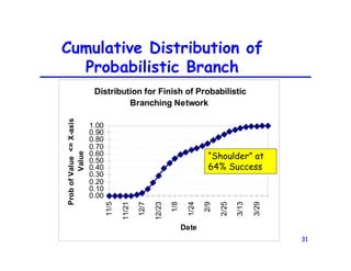
31. 31
Cumulative Distribution of
Probabilistic Branch
Distribution for Finish of Probabilistic
Branching Network
0.00
0.10
0.20
0.30
0.40
0.50
0.60
0.70
0.80
0.90
1.00
11/5
11/21
12/7
12/23
1/8
1/24
2/9
2/25
3/13
3/29
Date
Prob
of
Value
<=
X-axis
Value
“Shoulder” at
64% Success

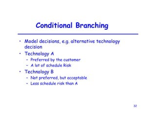
32. 32
Conditional Branching
• Model decisions, e.g. alternative technology
decision
• Technology A
– Preferred by the customer
– A lot of schedule Risk
• Technology B
– Not preferred, but acceptable
– Less schedule risk than A

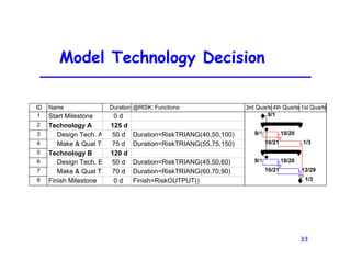
33. 33
Model Technology Decision
ID Name Duration @RISK: Functions
1 Start Milestone 0 d
2 Technology A 125 d
3 Design Tech. A 50 d Duration=RiskTRIANG(40,50,100)
4 Make & Qual T 75 d Duration=RiskTRIANG(55,75,150)
5 Technology B 120 d
6 Design Tech. B 50 d Duration=RiskTRIANG(45,50,60)
7 Make & Qual T 70 d Duration=RiskTRIANG(60,70,90)
8 Finish Milestone 0 d Finish=RiskOUTPUT()
9/1
9/1 10/20
10/21 1/3
9/1 10/20
10/21 12/29
1/3
3rd Quarte4th Quarte 1st Quarte

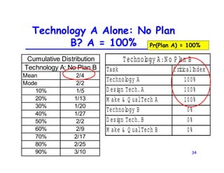
34. 34
Technology A Alone: No Plan
B? A = 100%
Task C riticalIndex
Technology A 100%
D esign Tech.A 100%
M ake & Q ualTech A 100%
Technology B 0%
D esign Tech.B 0%
M ake & Q ualTech B 0%
Technology A:N o P lan B
Mean 2/4
Mode 2/2
10% 1/5
20% 1/13
30% 1/20
40% 1/27
50% 2/2
60% 2/9
70% 2/17
80% 2/25
90% 3/10
Cumulative Distribution
Technology A: No Plan B
Pr(Plan A) = 100%

35. 35
If Technology A Design not
done by 10/25: Plan B
Unique I Name Duration @RISK: Functions
2 Start Milestone 0 d
8 Technology A 125 d
3 Design Tech. A 50 d Duration=RiskTRIANG(40,50,100);RiskIF(t3[Finish]>10/25/01,Branch=t7)
5 Make & Qual Tec 75 d Duration=RiskTRIANG(55,75,150)
9 Technology B 120 d
4 Design Tech. B 50 d Duration=RiskTRIANG(45,50,60)
6 Make & Qual Tec 70 d Duration=RiskTRIANG(60,70,90)
7 Finish Milestone 0 d Finish=RiskOUTPUT()

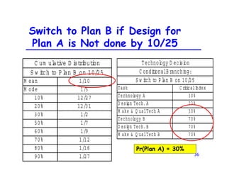
36. 36
Switch to Plan B if Design for
Plan A is Not done by 10/25
Task C riticalIndex
Technology A 30%
D esign Tech.A 23%
M ake & Q ualTech A 30%
Technology B 70%
D esign Tech.B 70%
M ake & Q ualTech B 70%
Technology D ecision
C onditionalB ranching:
S w itch to P lan B on 10/25
M ean 1/10
M ode 1/5
10% 12/27
20% 12/31
30% 1/2
50% 1/7
60% 1/9
70% 1/12
80% 1/16
90% 1/27
C um ul
ati
ve D i
stri
buti
on
S w i
tch to P l
an B on 10/25
Pr(Plan A) = 30%

37. 37
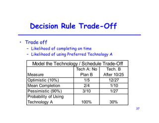
Decision Rule Trade-Off
• Trade off
– Likelihood of completing on time
– Likelihood of using Preferred Technology A
Measure
Tech A: No
Plan B
Tech. B
After 10/25
Optimistic (10%) 1/5 12/27
Mean Completion 2/4 1/10
Pessimistic (90%) 3/10 1/27
Probability of Using
Technology A 100% 30%
Model the Technology / Schedule Trade-Off

38. 38
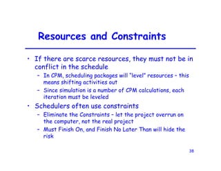
Resources and Constraints
• If there are scarce resources, they must not be in
conflict in the schedule
– In CPM, scheduling packages will “level” resources – this
means shifting activities out
– Since simulation is a number of CPM calculations, each
iteration must be leveled
• Schedulers often use constraints
– Eliminate the Constraints – let the project overrun on
the computer, not the real project
– Must Finish On, and Finish No Later Than will hide the
risk

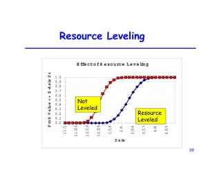
39. 39
Resource Leveling
E ffectofR esource Level
i
ng
0.0
0.1
0.2
0.3
0.4
0.5
0.6
0.7
0.8
0.9
1.0
1
1
/1
1
1
/2
0
1
2
/1
0
1
2
/2
9
1
/1
8
2
/6
2
/2
6
3
/1
7
4
/6
4
/2
5
D a te
P
ro
b
V
alu
e
<
=
X
-A
xis
D
a
Not
Leveled
Resource
Leveled

40. 40
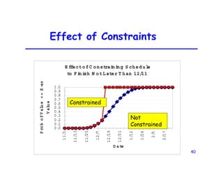
Effect of Constraints
E ffectofC onstrai
ni
ng S chedul
e
to Fi
ni
sh N otLater T han 12/
11
0.0
0.1
0.2
0.3
0.4
0.5
0.6
0.7
0.8
0.9
1.0
1
1
/1
1
1
/1
3
1
1
/2
5
1
2
/7
1
2
/1
9
1
2
/3
1
1
/1
2
1
/2
4
2
/5
2
/1
7
D a te
P
ro
b
o
f
V
alu
e
<
=
X
-ax
V
alu
e
Constrained
Not
Constrained