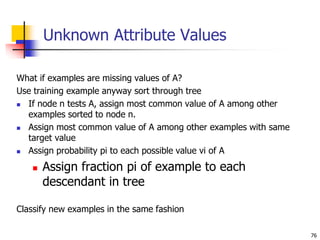
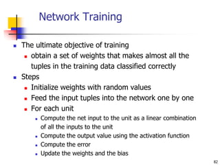
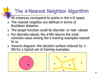
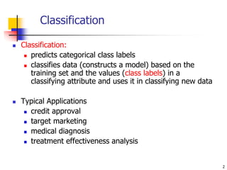
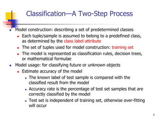
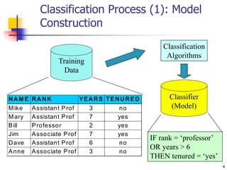
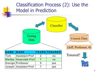
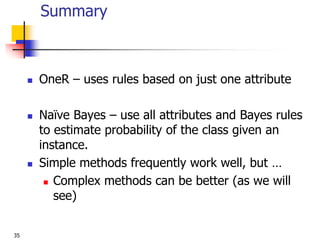
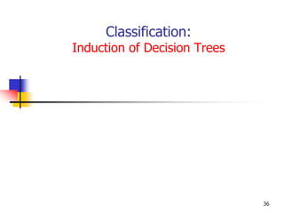
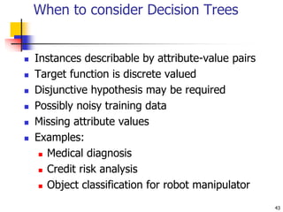
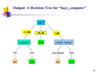
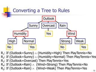
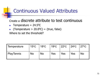
This document discusses classification, which is a type of supervised machine learning where algorithms are used to predict categorical class labels. There is a two-step process: 1) model construction using a training dataset to develop rules or formulas for classification, and 2) model usage to classify new data. Common applications include credit approval, target marketing, medical diagnosis, and treatment effectiveness analysis. The document also covers Bayesian classification, which uses probability distributions over class labels to classify new data instances based on attribute values and their probabilities.

1. 1
Classification

2. 2
 Classification:
 predicts categorical class labels
 classifies data (constructs a model) based on the
training set and the values (class labels) in a
classifying attribute and uses it in classifying new data
 Typical Applications
 credit approval
 target marketing
 medical diagnosis
 treatment effectiveness analysis
Classification

3. 3
Classification—A Two-Step Process
 Model construction: describing a set of predetermined classes
 Each tuple/sample is assumed to belong to a predefined class,
as determined by the class label attribute
 The set of tuples used for model construction: training set
 The model is represented as classification rules, decision trees,
or mathematical formulae
 Model usage: for classifying future or unknown objects
 Estimate accuracy of the model
 The known label of test sample is compared with the
classified result from the model
 Accuracy rate is the percentage of test set samples that are
correctly classified by the model
 Test set is independent of training set, otherwise over-fitting
will occur

4. 4
Classification Process (1): Model
Construction
Training
Data
NAME RANK YEARS TENURED
Mike Assistant Prof 3 no
Mary Assistant Prof 7 yes
Bill Professor 2 yes
Jim Associate Prof 7 yes
Dave Assistant Prof 6 no
Anne Associate Prof 3 no
Classification
Algorithms
IF rank = ‘professor’
OR years > 6
THEN tenured = ‘yes’
Classifier
(Model)

5. 5
Classification Process (2): Use the
Model in Prediction
Classifier
Testing
Data
NAME RANK YEARS TENURED
Tom Assistant Prof 2 no
Merlisa Associate Prof 7 no
George Professor 5 yes
Joseph Assistant Prof 7 yes
Unseen Data
(Jeff, Professor, 4)
Tenured?

6. 6
Supervised vs. Unsupervised
Learning
 Supervised learning (classification)
 Supervision: The training data (observations,
measurements, etc.) are accompanied by labels
indicating the class of the observations
 New data is classified based on the training set
 Unsupervised learning (clustering)
 The class labels of training data is unknown
 Given a set of measurements, observations, etc. with
the aim of establishing the existence of classes or
clusters in the data

7. 7
Issues regarding classification and
prediction (1): Data Preparation
 Data cleaning
 Preprocess data in order to reduce noise and handle
missing values
 Relevance analysis (feature selection)
 Remove the irrelevant or redundant attributes
 Data transformation
 Generalize and/or normalize data

8. 8
Issues regarding classification and prediction
(2): Evaluating Classification Methods
 Predictive accuracy
 Speed and scalability
 time to construct the model
 time to use the model
 Robustness
 handling noise and missing values
 Scalability
 efficiency in disk-resident databases
 Interpretability:
 understanding and insight provded by the model
 Goodness of rules
 decision tree size
 compactness of classification rules

9. 9
Simplicity first: 1R
 Simple algorithms often work very well!
 There are many kinds of simple structure, eg:
 One attribute does all the work
 All attributes contribute equally & independently
 A weighted linear combination might do
 Instance-based: use a few prototypes
 Use simple logical rules
 Success of method depends on the domain

10. 10
Inferring rudimentary rules
 1R: learns a 1-level decision tree
 I.e., rules that all test one particular attribute
 Basic version
 One branch for each value
 Each branch assigns most frequent class
 Error rate: proportion of instances that don’t belong to the
majority class of their corresponding branch
 Choose attribute with lowest error rate
(assumes nominal attributes)

11. 11
Pseudo-code for 1R
For each attribute,
For each value of the attribute, make a rule as follows:
count how often each class appears
find the most frequent class
make the rule assign that class to this attribute-value
Calculate the error rate of the rules
Choose the rules with the smallest error rate
 Note: “missing” is treated as a separate attribute value

12. 12
Evaluating the weather attributes
Attribute Rules Errors Total
errors
Outlook Sunny  No 2/5 4/14
Overcast  Yes 0/4
Rainy  Yes 2/5
Temp Hot  No* 2/4 5/14
Mild  Yes 2/6
Cool  Yes 1/4
Humidity High  No 3/7 4/14
Normal  Yes 1/7
Windy False  Yes 2/8 5/14
True  No* 3/6
Outlook Temp Humidity Windy Play
Sunny Hot High False No
Sunny Hot High True No
Overcast Hot High False Yes
Rainy Mild High False Yes
Rainy Cool Normal False Yes
Rainy Cool Normal True No
Overcast Cool Normal True Yes
Sunny Mild High False No
Sunny Cool Normal False Yes
Rainy Mild Normal False Yes
Sunny Mild Normal True Yes
Overcast Mild High True Yes
Overcast Hot Normal False Yes
Rainy Mild High True No
* indicates a tie

13. 13
Using Rules
Attribute Rules
Outlook Sunny  No
Overcast  Yes
Rainy  Yes
Outlook Temp. Humidity Windy Play
Sunny Cool High True ?
 A new day:

14. 14
Using Rules
Attribute Rules
Outlook Sunny  No
Overcast  Yes
Rainy  Yes
Outlook Temp. Humidity Windy Play
Sunny Cool High True No
 A new day:

15. 15
Dealing with
numeric attributes
 Discretize numeric attributes
 Divide each attribute’s range into intervals
 Sort instances according to attribute’s values
 Place breakpoints where the class changes
(the majority class)
 This minimizes the total error
 Example: temperature from weather data
64 65 68 69 70 71 72 72 75 75 80 81 83 85
Yes | No | Yes Yes Yes | No No No| Yes Yes | No | Yes Yes | No
Outlook Temperat
ure
Humidity Windy Play
Sunny 85 85 False No
Sunny 80 90 True No
Overcast 83 86 False Yes
Rainy 75 80 False Yes
… … … … …

16. 16
The problem of overfitting
 This procedure is very sensitive to noise
 One instance with an incorrect class label will probably
produce a separate interval
 Simple solution:
enforce minimum number of instances in majority
class per interval

17. 17
Discretization example
 Example (with min = 3):
 Final result for temperature attribute
64 65 68 69 70 71 72 72 75 75 80 81 83 85
Yes | No | Yes Yes Yes | No No Yes | Yes Yes | No | Yes Yes | No
64 65 68 69 70 71 72 72 75 75 80 81 83 85
Yes No Yes Yes Yes | No No Yes Yes Yes | No Yes Yes No

18. 18
With overfitting avoidance
 Resulting rule set:
Attribute Rules Errors Total errors
Outlook Sunny  No 2/5 4/14
Overcast  Yes 0/4
Rainy  Yes 2/5
Temperature  77.5  Yes 3/10 5/14
> 77.5  No* 2/4
Humidity  82.5  Yes 1/7 3/14
> 82.5 and  95.5  No 2/6
> 95.5  Yes 0/1
Windy False  Yes 2/8 5/14
True  No* 3/6

19. 20
Bayesian (Statistical) modeling
 “Opposite” of 1R: use all the attributes
 Two assumptions: Attributes are
 equally important
 statistically independent (given the class value)
 I.e., knowing the value of one attribute says nothing about
the value of another
(if the class is known)
 Independence assumption is almost never correct!
 But … this scheme works well in practice

20. 21
Probabilities for weather data
Outlook Temperature Humidity Windy Play
Yes No Yes No Yes No Yes No Yes No
Sunny 2 3 Hot 2 2 High 3 4 False 6 2 9 5
Overcast 4 0 Mild 4 2 Normal 6 1 True 3 3
Rainy 3 2 Cool 3 1
Sunny 2/9 3/5 Hot 2/9 2/5 High 3/9 4/5 False 6/9 2/5 9/14 5/14
Overcast 4/9 0/5 Mild 4/9 2/5 Normal 6/9 1/5 True 3/9 3/5
Rainy 3/9 2/5 Cool 3/9 1/5 Outlook Temp Humidity Windy Play
Sunny Hot High False No
Sunny Hot High True No
Overcast Hot High False Yes
Rainy Mild High False Yes
Rainy Cool Normal False Yes
Rainy Cool Normal True No
Overcast Cool Normal True Yes
Sunny Mild High False No
Sunny Cool Normal False Yes
Rainy Mild Normal False Yes
Sunny Mild Normal True Yes
Overcast Mild High True Yes
Overcast Hot Normal False Yes
Rainy Mild High True No

21. 22
Probabilities for weather data
Outlook Temp. Humidity Windy Play
Sunny Cool High True ?
 A new day:
Outlook Temperature Humidity Windy Play
Yes No Yes No Yes No Yes No Yes No
Sunny 2 3 Hot 2 2 High 3 4 False 6 2 9 5
Overcast 4 0 Mild 4 2 Normal 6 1 True 3 3
Rainy 3 2 Cool 3 1
Sunny 2/9 3/5 Hot 2/9 2/5 High 3/9 4/5 False 6/9 2/5 9/14 5/14
Overcast 4/9 0/5 Mild 4/9 2/5 Normal 6/9 1/5 True 3/9 3/5
Rainy 3/9 2/5 Cool 3/9 1/5

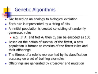
22. 23
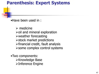
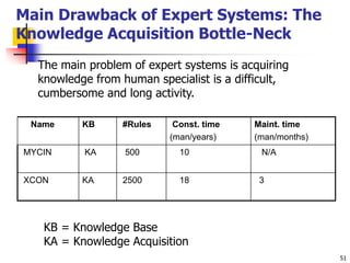
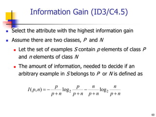
Bayes’s rule
 Probability of event H given evidence E :
 A priori probability of H :
 Probability of event before evidence is seen
 A posteriori probability of H :
 Probability of event after evidence is seen
]
Pr[
]
Pr[
]
|
Pr[
]
|
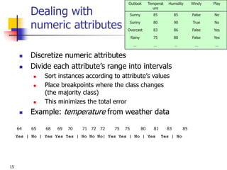
Pr[
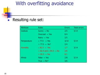
E
H
H
E
E
H 
]
|
Pr[ E
H
]
Pr[H
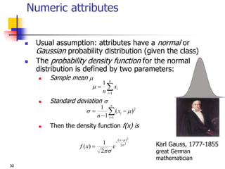
Thomas Bayes
Born: 1702 in London, England
Died: 1761 in Tunbridge Wells, Kent, England
from Bayes “Essay towards solving a problem in the
doctrine of chances” (1763)

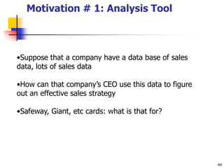
23. 24
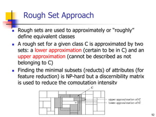
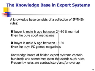
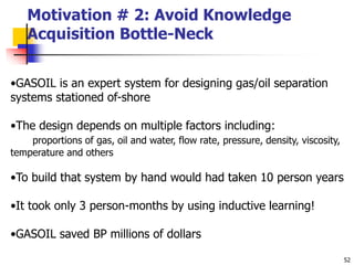
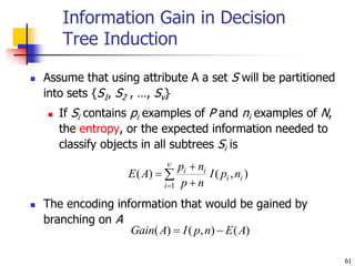
Naïve Bayes for classification
 Classification learning: what’s the probability of the
class given an instance?
 Evidence E = instance
 Event H = class value for instance
 Naïve assumption: evidence splits into parts (i.e.
attributes) that are independent
]
Pr[
]
Pr[
]
|
Pr[
]
|
Pr[
]
|
Pr[
]
|
Pr[ 2
1
E
H
H
E
H
E
H
E
E
H n



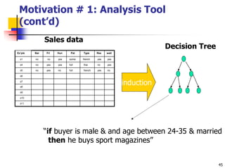
24. 25
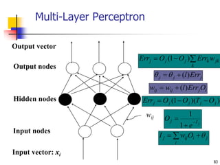
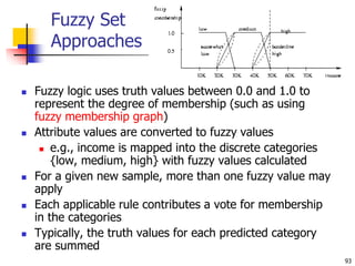
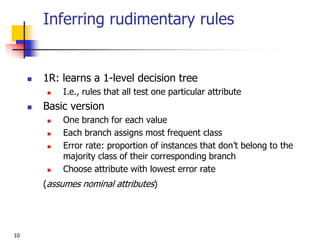
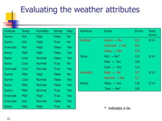
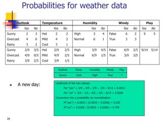
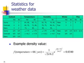
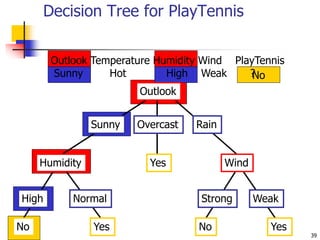
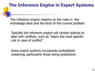
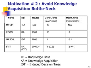
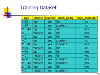
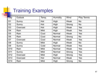
Weather data example
Outlook Temp. Humidity Windy Play
Sunny Cool High True ?
Evidence E
Probability of
class “yes”
]
|
Pr[
]
|
Pr[ yes
Sunny
Outlook
E
yes 

]
|
Pr[ yes
Cool
e
Temperatur 

]
|
Pr[ yes
High
Humidity 

]
|
Pr[ yes
True
Windy 

]
Pr[
]
Pr[
E
yes

]
Pr[
14
9
9
3
9
3
9
3
9
2
E






25. 26
Probabilities for weather data
Outlook Temp. Humidity Windy Play
Sunny Cool High True ?
 A new day: Likelihood of the two classes
For “yes” = 2/9  3/9  3/9  3/9  9/14 = 0.0053
For “no” = 3/5  1/5  4/5  3/5  5/14 = 0.0206
Conversion into a probability by normalization:
P(“yes”) = 0.0053 / (0.0053 + 0.0206) = 0.205
P(“no”) = 0.0206 / (0.0053 + 0.0206) = 0.795
Outlook Temperature Humidity Windy Play
Yes No Yes No Yes No Yes No Yes No
Sunny 2 3 Hot 2 2 High 3 4 False 6 2 9 5
Overcast 4 0 Mild 4 2 Normal 6 1 True 3 3
Rainy 3 2 Cool 3 1
Sunny 2/9 3/5 Hot 2/9 2/5 High 3/9 4/5 False 6/9 2/5 9/14 5/14
Overcast 4/9 0/5 Mild 4/9 2/5 Normal 6/9 1/5 True 3/9 3/5
Rainy 3/9 2/5 Cool 3/9 1/5

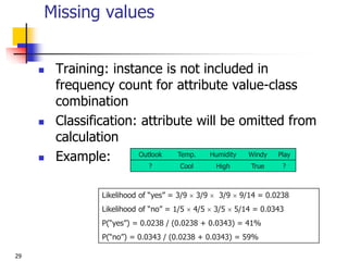
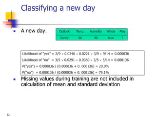
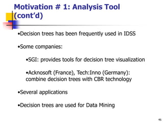
26. 27
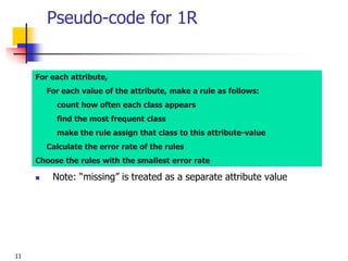
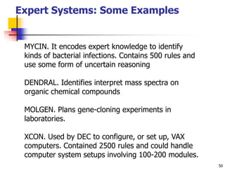
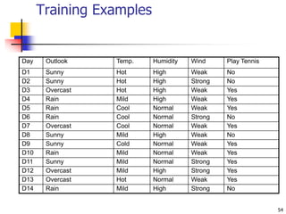
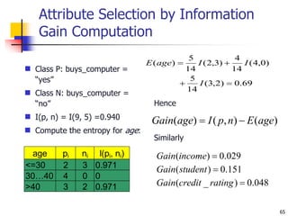
The “zero-frequency problem”
 What if an attribute value doesn’t occur with every class
value?
(e.g. “Humidity = high” for class “yes”)
 Probability will be zero!
 A posteriori probability will also be zero!
(No matter how likely the other values are!)
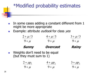
 Remedy: add 1 to the count for every attribute value-class
combination (Laplace estimator)
 Result: probabilities will never be zero!
(also: stabilizes probability estimates)
0
]
|
Pr[ 
E
yes
0
]
|
Pr[ 
 yes
High
Humidity

27. 28
*Modified probability estimates
 In some cases adding a constant different from 1
might be more appropriate
 Example: attribute outlook for class yes
 Weights don’t need to be equal
(but they must sum to 1)




9
3
/
2




9
3
/
4




9
3
/
3
Sunny Overcast Rainy




9
2 1
p




9
4 2
p




9
3 3
p

28. 29
Missing values
 Training: instance is not included in
frequency count for attribute value-class
combination
 Classification: attribute will be omitted from
calculation
 Example: Outlook Temp. Humidity Windy Play
? Cool High True ?
Likelihood of “yes” = 3/9  3/9  3/9  9/14 = 0.0238
Likelihood of “no” = 1/5  4/5  3/5  5/14 = 0.0343
P(“yes”) = 0.0238 / (0.0238 + 0.0343) = 41%
P(“no”) = 0.0343 / (0.0238 + 0.0343) = 59%

29. 30
Numeric attributes
 Usual assumption: attributes have a normal or
Gaussian probability distribution (given the class)
 The probability density function for the normal
distribution is defined by two parameters:
 Sample mean 
 Standard deviation 
 Then the density function f(x) is



n
i
i
x
n 1
1






n
i
i
x
n 1
2
)
(
1
1


2
2
2
)
(
2
1
)
( 






x
e
x
f Karl Gauss, 1777-1855
great German
mathematician

30. 31
Statistics for
weather data
 Example density value:
0340
.
0
2
.
6
2
1
)
|
66
(
2
2
2
.
6
2
)
73
66
(


 


e
yes
e
temperatur
f

Outlook Temperature Humidity Windy Play
Yes No Yes No Yes No Yes No Yes No
Sunny 2 3 64, 68, 65, 71, 65, 70, 70, 85, False 6 2 9 5
Overcast 4 0 69, 70, 72, 80, 70, 75, 90, 91, True 3 3
Rainy 3 2 72, … 85, … 80, … 95, …
Sunny 2/9 3/5  =73  =75  =79  =86 False 6/9 2/5 9/14 5/14
Overcast 4/9 0/5  =6.2  =7.9  =10.2  =9.7 True 3/9 3/5
Rainy 3/9 2/5

31. 32
Classifying a new day
 A new day:
 Missing values during training are not included in
calculation of mean and standard deviation
Outlook Temp. Humidity Windy Play
Sunny 66 90 true ?
Likelihood of “yes” = 2/9  0.0340  0.0221  3/9  9/14 = 0.000036
Likelihood of “no” = 3/5  0.0291  0.0380  3/5  5/14 = 0.000136
P(“yes”) = 0.000036 / (0.000036 + 0. 000136) = 20.9%
P(“no”) = 0.000136 / (0.000036 + 0. 000136) = 79.1%

32. 33
Naïve Bayes: discussion
 Naïve Bayes works surprisingly well (even if
independence assumption is clearly violated)
 Why? Because classification doesn’t require
accurate probability estimates as long as
maximum probability is assigned to correct
class
 However: adding too many redundant
attributes will cause problems (e.g. identical
attributes)
 Note also: many numeric attributes are not
normally distributed .

33. Naïve Bayes Extensions
 Improvements:
 select best attributes (e.g. with greedy
search)
 often works as well or better with just a
fraction of all attributes
 Bayesian Networks

34. 35
Summary
 OneR – uses rules based on just one attribute
 Naïve Bayes – use all attributes and Bayes rules
to estimate probability of the class given an
instance.
 Simple methods frequently work well, but …
 Complex methods can be better (as we will
see)

35. Classification:
Induction of Decision Trees
36

36. 37
Decision Tree for PlayTennis
Outlook
Sunny Overcast Rain
Humidity
High Normal
Wind
Strong Weak
No Yes
Yes
Yes
No
Outlook Temp. Humidity Windy Play
Sunny Cool High True ?

37. 38
Decision Tree for PlayTennis
Outlook
Sunny Overcast Rain
Humidity
High Normal
No Yes
Each internal node tests an attribute
Each branch corresponds to an
attribute value node
Each leaf node assigns a classification

38. 39
No
Decision Tree for PlayTennis
Outlook
Sunny Overcast Rain
Humidity
High Normal
Wind
Strong Weak
No Yes
Yes
Yes
No
Outlook Temperature Humidity Wind PlayTennis
Sunny Hot High Weak ?

39. 40
Decision Tree for Conjunction
Outlook
Sunny Overcast Rain
Wind
Strong Weak
No Yes
No
Outlook=Sunny  Wind=Weak
No

40. 41
Decision Tree for Disjunction
Outlook
Sunny Overcast Rain
Yes
Outlook=Sunny  Wind=Weak
Wind
Strong Weak
No Yes
Wind
Strong Weak
No Yes

41. 42
Decision Tree
Outlook
Sunny Overcast Rain
Humidity
High Normal
Wind
Strong Weak
No Yes
Yes
Yes
No
• decision trees represent disjunctions of conjunctions
(Outlook=Sunny  Humidity=Normal)
 (Outlook=Overcast)
 (Outlook=Rain  Wind=Weak)

42. 43
When to consider Decision Trees
 Instances describable by attribute-value pairs
 Target function is discrete valued
 Disjunctive hypothesis may be required
 Possibly noisy training data
 Missing attribute values
 Examples:
 Medical diagnosis
 Credit risk analysis
 Object classification for robot manipulator

43. 44
Motivation # 1: Analysis Tool
•Suppose that a company have a data base of sales
data, lots of sales data
•How can that company’s CEO use this data to figure
out an effective sales strategy
•Safeway, Giant, etc cards: what is that for?

44. 45
Motivation # 1: Analysis Tool
(cont’d)
Ex’ple Bar Fri Hun Pat Type Res wait
x1 no no yes some french yes yes
x4 no yes yes full thai no yes
x5 no yes no full french yes no
x6
x7
x8
x9
x10
x11
Sales data
“if buyer is male & and age between 24-35 & married
then he buys sport magazines”
induction
Decision Tree

45. 46
Motivation # 1: Analysis Tool
(cont’d)
•Decision trees has been frequently used in IDSS
•Some companies:
•SGI: provides tools for decision tree visualization
•Acknosoft (France), Tech:Inno (Germany):
combine decision trees with CBR technology
•Several applications
•Decision trees are used for Data Mining

46. 47
Parenthesis: Expert Systems
•Have been used in :
 medicine
oil and mineral exploration
weather forecasting
stock market predictions
financial credit, fault analysis
some complex control systems
•Two components:
Knowledge Base
Inference Engine

47. 48
The Knowledge Base in Expert Systems
A knowledge base consists of a collection of IF-THEN
rules:
if buyer is male & age between 24-50 & married
then he buys sport magazines
if buyer is male & age between 18-30
then he buys PC games magazines
Knowledge bases of fielded expert systems contain
hundreds and sometimes even thousands such rules.
Frequently rules are contradictory and/or overlap

48. 49
The Inference Engine in Expert Systems
The inference engine reasons on the rules in the
knowledge base and the facts of the current problem
Typically the inference engine will contain policies to
deal with conflicts, such as “select the most specific
rule in case of conflict”
Some expert systems incorporate probabilistic
reasoning, particularly those doing predictions

49. 50
Expert Systems: Some Examples
MYCIN. It encodes expert knowledge to identify
kinds of bacterial infections. Contains 500 rules and
use some form of uncertain reasoning
DENDRAL. Identifies interpret mass spectra on
organic chemical compounds
MOLGEN. Plans gene-cloning experiments in
laboratories.
XCON. Used by DEC to configure, or set up, VAX
computers. Contained 2500 rules and could handle
computer system setups involving 100-200 modules.

50. 51
Main Drawback of Expert Systems: The
Knowledge Acquisition Bottle-Neck
The main problem of expert systems is acquiring
knowledge from human specialist is a difficult,
cumbersome and long activity.
Name KB #Rules Const. time
(man/years)
Maint. time
(man/months)
MYCIN KA 500 10 N/A
XCON KA 2500 18 3
KB = Knowledge Base
KA = Knowledge Acquisition

51. 52
Motivation # 2: Avoid Knowledge
Acquisition Bottle-Neck
•GASOIL is an expert system for designing gas/oil separation
systems stationed of-shore
•The design depends on multiple factors including:
proportions of gas, oil and water, flow rate, pressure, density, viscosity,
temperature and others
•To build that system by hand would had taken 10 person years
•It took only 3 person-months by using inductive learning!
•GASOIL saved BP millions of dollars

52. 53
Motivation # 2 : Avoid Knowledge
Acquisition Bottle-Neck
Name KB #Rules Const. time
(man/years)
Maint. time
(man/months)
MYCIN KA 500 10 N/A
XCON KA 2500 18 3
GASOIL IDT 2800 1 0.1
BMT KA
(IDT)
30000+ 9 (0.3) 2 (0.1)
KB = Knowledge Base
KA = Knowledge Acquisition
IDT = Induced Decision Trees

53. 54
Training Examples
Day Outlook Temp. Humidity Wind Play Tennis
D1 Sunny Hot High Weak No
D2 Sunny Hot High Strong No
D3 Overcast Hot High Weak Yes
D4 Rain Mild High Weak Yes
D5 Rain Cool Normal Weak Yes
D6 Rain Cool Normal Strong No
D7 Overcast Cool Normal Weak Yes
D8 Sunny Mild High Weak No
D9 Sunny Cold Normal Weak Yes
D10 Rain Mild Normal Weak Yes
D11 Sunny Mild Normal Strong Yes
D12 Overcast Mild High Strong Yes
D13 Overcast Hot Normal Weak Yes
D14 Rain Mild High Strong No

54. 55
Temp
Cool Mild Hot
Wind
Strong Weak
No
Outlook
Outlook
Sunny
Overcast
Yes
Yes
Wind
Strong Weak
Yes
No
Yes
No
Humidity
High
Normal
Outlook
Sunny Overcast
Yes
Tree 1
Yes
No
Humidity
High
Normal
Outlook
Sunny Overcast
Yes
Sunny Rain
Rain

55. 56
Outlook
Sunny Overcast Rain
Humidity
High Normal
Wind
Strong Weak
No Yes
Yes
Yes
No
Tree 2

56. 57
Top-Down Induction of Decision
Trees ID3
1. A  the “best” decision attribute for next node
2. Assign A as decision attribute for node
3. For each value of A create new descendant
4. Sort training examples to leaf node according to
the attribute value of the branch
5. If all training examples are perfectly classified
(same value of target attribute) stop, else
iterate over new leaf nodes.

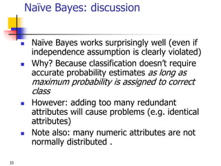
57. 58
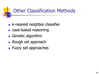
Which Attribute is ”best”?
A1=?
True False
[21+, 5-] [8+, 30-]
[29+,35-] A2=?
True False
[18+, 33-] [11+, 2-]
[29+,35-]

58. 59
Entropy
 S is a sample of training examples
 p+ is the proportion of positive examples
 p- is the proportion of negative examples
 Entropy measures the impurity of S
Entropy(S) = -p+ log2 p+ - p- log2 p-

59. 60
Information Gain (ID3/C4.5)
 Select the attribute with the highest information gain
 Assume there are two classes, P and N
 Let the set of examples S contain p elements of class P
and n elements of class N
 The amount of information, needed to decide if an
arbitrary example in S belongs to P or N is defined as
n
p
n
n
p
n
n
p
p
n
p
p
n
p
I






 2
2 log
log
)
,
(

60. 61
Information Gain in Decision
Tree Induction
 Assume that using attribute A a set S will be partitioned
into sets {S1, S2 , …, Sv}
 If Si contains pi examples of P and ni examples of N,
the entropy, or the expected information needed to
classify objects in all subtrees Si is
 The encoding information that would be gained by
branching on A

 



1
)
,
(
)
(
i
i
i
i
i
n
p
I
n
p
n
p
A
E
)
(
)
,
(
)
( A
E
n
p
I
A
Gain 


61. 62
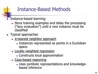
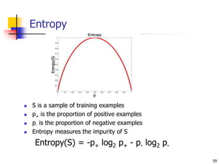
Information Gain
 Gain(S,A): expected reduction in entropy due to sorting S on
attribute A
A1=?
True False
[21+, 5-] [8+, 30-]
[29+,35-] A2=?
True False
[18+, 33-] [11+, 2-]
[29+,35-]
Gain(S,A)=Entropy(S) - vvalues(A) |Sv|/|S| Entropy(Sv)
Entropy([29+,35-]) = -29/64 log2 29/64 – 35/64 log2 35/64
= 0.99

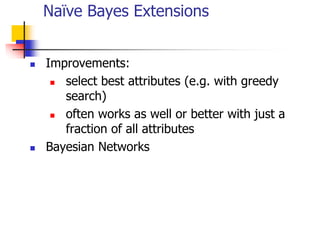
62. 63
Information Gain
A1=?
True False
[21+, 5-] [8+, 30-]
[29+,35-]
Entropy([21+,5-]) = 0.71
Entropy([8+,30-]) = 0.74
Gain(S,A1)=Entropy(S)
-26/64*Entropy([21+,5-])
-38/64*Entropy([8+,30-])
=0.27
Entropy([18+,33-]) = 0.94
Entropy([8+,30-]) = 0.62
Gain(S,A2)=Entropy(S)
-51/64*Entropy([18+,33-])
-13/64*Entropy([11+,2-])
=0.12
A2=?
True False
[18+, 33-] [11+, 2-]
[29+,35-]

63. 64
Training Dataset
age income student credit_rating buys_computer
<=30 high no fair no
<=30 high no excellent no
31…40 high no fair yes
>40 medium no fair yes
>40 low yes fair yes
>40 low yes excellent no
31…40 low yes excellent yes
<=30 medium no fair no
<=30 low yes fair yes
>40 medium yes fair yes
<=30 medium yes excellent yes
31…40 medium no excellent yes
31…40 high yes fair yes
>40 medium no excellent no

64. 65
Attribute Selection by Information
Gain Computation
 Class P: buys_computer =
“yes”
 Class N: buys_computer =
“no”
 I(p, n) = I(9, 5) =0.940
 Compute the entropy for age:
Hence
Similarly
age pi ni I(pi, ni)
<=30 2 3 0.971
30…40 4 0 0
>40 3 2 0.971
69
.
0
)
2
,
3
(
14
5
)
0
,
4
(
14
4
)
3
,
2
(
14
5
)
(




I
I
I
age
E
048
.
0
)
_
(
151
.
0
)
(
029
.
0
)
(



rating
credit
Gain
student
Gain
income
Gain
)
(
)
,
(
)
( age
E
n
p
I
age
Gain 


65. 66
Output: A Decision Tree for “buys_computer”
age?
overcast
student? credit rating?
no yes fair
excellent
<=30 >40
no no
yes yes
yes
30..40

66. 67
Training Examples
Day Outlook Temp. Humidity Wind Play Tennis
D1 Sunny Hot High Weak No
D2 Sunny Hot High Strong No
D3 Overcast Hot High Weak Yes
D4 Rain Mild High Weak Yes
D5 Rain Cool Normal Weak Yes
D6 Rain Cool Normal Strong No
D7 Overcast Cool Normal Weak Yes
D8 Sunny Mild High Weak No
D9 Sunny Cold Normal Weak Yes
D10 Rain Mild Normal Weak Yes
D11 Sunny Mild Normal Strong Yes
D12 Overcast Mild High Strong Yes
D13 Overcast Hot Normal Weak Yes
D14 Rain Mild High Strong No

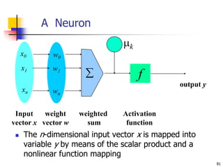
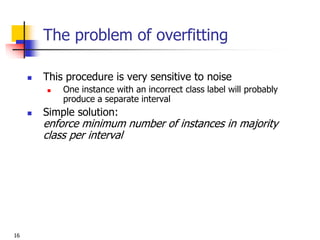
67. 68
Selecting the Next Attribute
Humidity
High Normal
[3+, 4-] [6+, 1-]
S=[9+,5-]
E=0.940
Gain(S,Humidity)
=0.940-(7/14)*0.985
– (7/14)*0.592
=0.151
E=0.985 E=0.592
Wind
Weak Strong
[6+, 2-] [3+, 3-]
S=[9+,5-]
E=0.940
E=0.811 E=1.0
Gain(S,Wind)
=0.940-(8/14)*0.811
– (6/14)*1.0
=0.048

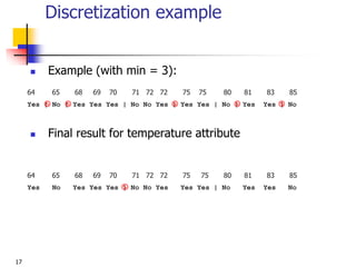
68. 69
Selecting the Next Attribute
Outlook
Sunny Rain
[2+, 3-] [3+, 2-]
S=[9+,5-]
E=0.940
Gain(S,Outlook)
=0.940-(5/14)*0.971
-(4/14)*0.0 – (5/14)*0.0971
=0.247
E=0.971 E=0.971
Over
cast
[4+, 0]
E=0.0
Temp ?

69. 70
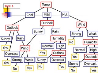
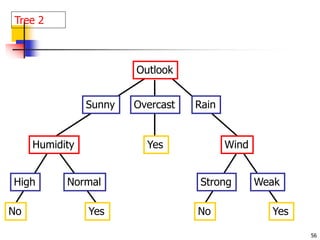
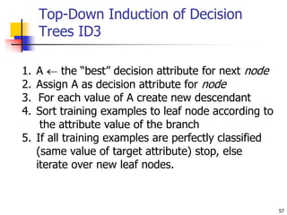
ID3 Algorithm
Outlook
Sunny Overcast Rain
Yes
[D1,D2,…,D14]
[9+,5-]
Ssunny=[D1,D2,D8,D9,D11]
[2+,3-]
? ?
[D3,D7,D12,D13]
[4+,0-]
[D4,D5,D6,D10,D14]
[3+,2-]
Gain(Ssunny , Humidity)=0.970-(3/5)0.0 – 2/5(0.0) = 0.970
Gain(Ssunny , Temp.)=0.970-(2/5)0.0 –2/5(1.0)-(1/5)0.0 = 0.570
Gain(Ssunny , Wind)=0.970= -(2/5)1.0 – 3/5(0.918) = 0.019

70. 71
ID3 Algorithm
Outlook
Sunny Overcast Rain
Humidity
High Normal
Wind
Strong Weak
No Yes
Yes
Yes
No
[D3,D7,D12,D13]
[D8,D9,D11] [D6,D14]
[D1,D2] [D4,D5,D10]

71. 72
Converting a Tree to Rules
Outlook
Sunny Overcast Rain
Humidity
High Normal
Wind
Strong Weak
No Yes
Yes
Yes
No
R1: If (Outlook=Sunny)  (Humidity=High) Then PlayTennis=No
R2: If (Outlook=Sunny)  (Humidity=Normal) Then PlayTennis=Yes
R3: If (Outlook=Overcast) Then PlayTennis=Yes
R4: If (Outlook=Rain)  (Wind=Strong) Then PlayTennis=No
R5: If (Outlook=Rain)  (Wind=Weak) Then PlayTennis=Yes

72. 73
Continuous Valued Attributes
Create a discrete attribute to test continuous
 Temperature = 24.50C
 (Temperature > 20.00C) = {true, false}
Where to set the threshold?
Temperature 150C 180C 190C 220C 240C 270C
PlayTennis No No Yes Yes Yes No

73. 74
Attributes with many Values
 Problem: if an attribute has many values, maximizing InformationGain
will select it.
 E.g.: Imagine using Date=12.7.1996 as attribute
perfectly splits the data into subsets of size 1
Use GainRatio instead of information gain as criteria:
GainRatio(S,A) = Gain(S,A) / SplitInformation(S,A)
SplitInformation(S,A) = -i=1..c |Si|/|S| log2 |Si|/|S|
Where Si is the subset for which attribute A has the value vi

74. 75
Attributes with Cost
Consider:
 Medical diagnosis : blood test costs 1000 SEK
 Robotics: width_from_one_feet has cost 23 secs.
How to learn a consistent tree with low expected
cost?
Replace Gain by :
Gain2(S,A)/Cost(A) [Tan, Schimmer 1990]
2Gain(S,A)-1/(Cost(A)+1)w w [0,1] [Nunez 1988]

75. 76
Unknown Attribute Values
What if examples are missing values of A?
Use training example anyway sort through tree
 If node n tests A, assign most common value of A among other
examples sorted to node n.
 Assign most common value of A among other examples with same
target value
 Assign probability pi to each possible value vi of A
 Assign fraction pi of example to each
descendant in tree
Classify new examples in the same fashion

76. 77
MS

77. 78

78. 79
Classification by backpropagation

79. 80
Neural Networks
 Advantages
 prediction accuracy is generally high
 robust, works when training examples contain errors
 output may be discrete, real-valued, or a vector of
several discrete or real-valued attributes
 fast evaluation of the learned target function
 Criticism
 long training time
 difficult to understand the learned function (weights)
 not easy to incorporate domain knowledge

80. 81
A Neuron
 The n-dimensional input vector x is mapped into
variable y by means of the scalar product and a
nonlinear function mapping
k
-
f
weighted
sum
Input
vector x
output y
Activation
function
weight
vector w

w0
w1
wn
x0
x1
xn

81. Network Training
 The ultimate objective of training
 obtain a set of weights that makes almost all the
tuples in the training data classified correctly
 Steps
 Initialize weights with random values
 Feed the input tuples into the network one by one
 For each unit
 Compute the net input to the unit as a linear combination
of all the inputs to the unit
 Compute the output value using the activation function
 Compute the error
 Update the weights and the bias
82

82. Multi-Layer Perceptron
Output nodes
Input nodes
Hidden nodes
Output vector
Input vector: xi
wij
 

i
j
i
ij
j O
w
I 
j
I
j
e
O 


1
1
)
)(
1
( j
j
j
j
j O
T
O
O
Err 


jk
k
k
j
j
j w
Err
O
O
Err 

 )
1
(
i
j
ij
ij O
Err
l
w
w )
(


j
j
j Err
l)
(



83

83. 85
Other Classification Methods
 k-nearest neighbor classifier
 case-based reasoning
 Genetic algorithm
 Rough set approach
 Fuzzy set approaches

84. 86
Instance-Based Methods
 Instance-based learning:
 Store training examples and delay the processing
(“lazy evaluation”) until a new instance must be
classified
 Typical approaches
 k-nearest neighbor approach
 Instances represented as points in a Euclidean
space.
 Locally weighted regression
 Constructs local approximation
 Case-based reasoning
 Uses symbolic representations and knowledge-
based inference

85. 87
The k-Nearest Neighbor Algorithm
 All instances correspond to points in the n-D space.
 The nearest neighbor are defined in terms of
Euclidean distance.
 The target function could be discrete- or real- valued.
 For discrete-valued, the k-NN returns the most
common value among the k training examples nearest
to xq.
 Vonoroi diagram: the decision surface induced by 1-
NN for a typical set of training examples.
.
_
+
_ xq
+
_ _
+
_
_
+
.
.
.
. .

86. 88
Discussion on the k-NN Algorithm
 The k-NN algorithm for continuous-valued target functions
 Calculate the mean values of the k nearest neighbors
 Distance-weighted nearest neighbor algorithm
 Weight the contribution of each of the k neighbors
according to their distance to the query point xq
 giving greater weight to closer neighbors
 Similarly, for real-valued target functions
 Robust to noisy data by averaging k-nearest neighbors
 Curse of dimensionality: distance between neighbors could
be dominated by irrelevant attributes.
 To overcome it, axes stretch or elimination of the least
relevant attributes.
w
d xq xi
 1
2
( , )

87. 89
Case-Based Reasoning
 Also uses: lazy evaluation + analyze similar instances
 Difference: Instances are not “points in a Euclidean space”
 Example: Water faucet problem in CADET (Sycara et al’92)
 Methodology
 Instances represented by rich symbolic descriptions
(e.g., function graphs)
 Multiple retrieved cases may be combined
 Tight coupling between case retrieval, knowledge-based
reasoning, and problem solving
 Research issues
 Indexing based on syntactic similarity measure, and
when failure, backtracking, and adapting to additional
cases

88. 90
Remarks on Lazy vs. Eager Learning
 Instance-based learning: lazy evaluation
 Decision-tree and Bayesian classification: eager evaluation
 Key differences
 Lazy method may consider query instance xq when deciding how to
generalize beyond the training data D
 Eager method cannot since they have already chosen global
approximation when seeing the query
 Efficiency: Lazy - less time training but more time predicting
 Accuracy
 Lazy method effectively uses a richer hypothesis space since it uses
many local linear functions to form its implicit global approximation
to the target function
 Eager: must commit to a single hypothesis that covers the entire
instance space

89. 91
Genetic Algorithms
 GA: based on an analogy to biological evolution
 Each rule is represented by a string of bits
 An initial population is created consisting of randomly
generated rules
 e.g., IF A1 and Not A2 then C2 can be encoded as 100
 Based on the notion of survival of the fittest, a new
population is formed to consists of the fittest rules and
their offsprings
 The fitness of a rule is represented by its classification
accuracy on a set of training examples
 Offsprings are generated by crossover and mutation

90. 92
Rough Set Approach
 Rough sets are used to approximately or “roughly”
define equivalent classes
 A rough set for a given class C is approximated by two
sets: a lower approximation (certain to be in C) and an
upper approximation (cannot be described as not
belonging to C)
 Finding the minimal subsets (reducts) of attributes (for
feature reduction) is NP-hard but a discernibility matrix
is used to reduce the computation intensity

91. 93
Fuzzy Set
Approaches
 Fuzzy logic uses truth values between 0.0 and 1.0 to
represent the degree of membership (such as using
fuzzy membership graph)
 Attribute values are converted to fuzzy values
 e.g., income is mapped into the discrete categories
{low, medium, high} with fuzzy values calculated
 For a given new sample, more than one fuzzy value may
apply
 Each applicable rule contributes a vote for membership
in the categories
 Typically, the truth values for each predicted category
are summed