This document provides an overview of demand, supply, and market equilibrium. It discusses key concepts such as: - The law of demand which states that as price increases, quantity demanded decreases, assuming all other factors stay constant. - Supply functions which show the relationship between quantity supplied and price when other factors are held fixed. The law of supply states that quantity supplied rises with price. - Market equilibrium which occurs where quantity demanded equals quantity supplied, establishing an equilibrium price. - Elasticities including price elasticity of demand, income elasticity of demand, and cross elasticity of demand which measure responsiveness of demand to changes in price, income, and prices of related goods.

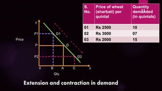
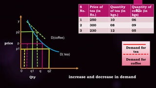
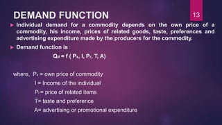
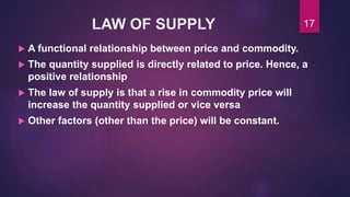
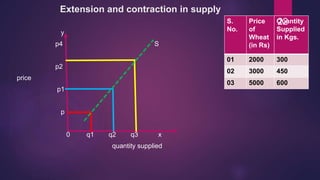
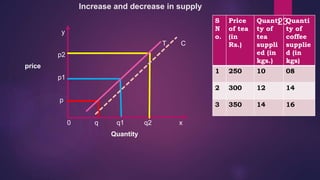
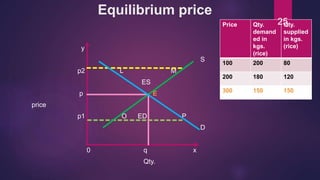
1. DEMAND &
SUPPLY
A GLANCE
07/03/2015
1

2. Introduction
 Two major forces
 What, how, when, where, whom aspects are covered
 Interaction decides price
 Response of households and buyers
 Market and competition are integral part
 Producers and sellers
 Utility is also associated
 Social well being
2

3. DEMAND
THE BASE OF ECONOMY
3

4. Meaning
 The amount that a consumer
will purchase and will use over
a period of time at a given
price
 It covers:
i. Desire
ii. utility
iii. Ability to pay / purchasing
power
iv. Ready to pay a given price
 Every factor is individually
effective:
i. Taste, preference, desires
ii. consumption level
iii. Time factor
iv. Market
v. Income
vi. Availability of substitute and
complementary goods
vii. Prices
viii. Distribution channels
4

5. LAW OF DEMAND
 The law of demand expresses the functional relationship
between price and quantity demanded.
 Assumption of ‘ Ceteris Paribus’. A hypothetical
assumption
 If price of a commodity falls, the quantity demanded of it
will rise and vice versa.
 Inverse relationship between price and quantity
 Other factors also play an important role.
 Real world variables.
5

6. RELATIONSHIP
Other things
being equal
price
Quantity
6

7. Market demand Aggregate demand
 Market demand is the sum total
of demands of all consumers in
the market for a commodity at
a various price levels at a point
of time.
 It is a micro economic term.
 It is calculated by adding up all
the quantities demanded over a
period by all the consumers (
homogeneity is required)
 Aggregate demand is the total
of all the demand for all the
goods and services at various
prices levels in an economy
over a period of time.
 It is macro economic term.
 It is a demand for GDP and
hence, consumption
expenditure, investment, govt.
expenditure on capital goods
and net exports.
7

8. Factors Exceptions
 Taste and preferences
 Income
 Related goods
 Complementary goods
 Consumer market
 Expectations of consumers
 Regional factors
 Govt. policies
 Income distribution
 Climatic conditions
 High value products
 Giffen goods
 False expectations for future
 Human ignorance
8

9. ASSUMPTIONS
 No change in tastes n preferences over a
period of time.
 Income is constant over a period of time.
 Related good’s prices will not change
 Given time period
9

10. MOVEMENT AND SHIFT ALONG DEMAND
CURVE
Movement in demand occurs because of extension and
contraction of demand. It occurs because of rise or fall in
commodity prices over a period of time (other factors are said
to be equal).
Shift in demand occurs because of increase and decrease
in demand. It occurs when there is a change in demand
because of the changes in other factors other than the price.
Prices of related goods, expectations of consumers, rainfall
etc. are some of the reasons for shift.
10

11. y
P1 D1
Price
P D
P2 D2
0 B A C x
Qty.
S.
No.
Price of wheat
(sharbati) per
quintal
Quantity
demanded
(in quintals)
01 Rs 2500 10
02 Rs 3000 07
03 Rs 2000 15
11

12. y
p2
D(coffee)
price p
p1
D( tea)
0 q1 q q2
Qty increase and decrease in demand
S
No.
Price of
tea (in
Rs.)
Quantity
of tea (in
kgs.)
Quantity of
coffee (in
kgs)
1 250 10 06
2 300 08 09
3 230 12 05
Demand for
tea
Demand for
coffee
12

13. DEMAND FUNCTION
 Individual demand for a commodity depends on the own price of a
commodity, his income, prices of related goods, taste, preferences and
advertising expenditure made by the producers for the commodity.
 Demand function is :
Qd = f ( Px, I, Pr, T, A)
where, Px = own price of commodity
I = Income of the individual
Pr = price of related items
T= taste and preference
A= advertising or promotional expenditure
13

14. IMPLICATIONS OF DEMAND
FUNCTION
 This is an individual demand function
 Other factors are remained constant
 Price is held to be an independent but effective variable
 It has a direct relationship with shift and movement along the demand curve
 It is a general function, where the quantity demanded will change with
change in price.
 It can be linear if the utility derived from commodities doesn’t satisfy the
consumers or sometimes a price increase in daily products increases its
demand.
14

15. SUPPLY
 It is a flow concept
 It refers to the amount of a commodity that the firms produce and offer for
sale in the market over a period of time.
 Time is an important ingredient.
 Quantity supplied is not related with quantity sold.
 It shows the relationship between price of a commodity and the quantity
supplied at various possible prices.
 Hence, supply refers to the quantity of the commodity which a firm are
able and willing to sell at particular price.
15

16. SUPPLY FUNCTION
 Supply of a commodity involves various factors
 It can be price of the commodity, price of inputs, state of technology,
competitors, price of related goods and future expectations, future
contingencies.
Qs = fS ( Px, f1, f2, …..fm, T, C)
where, Qs = quantity supplied
Px = price
f 1 to fm = prices of various inputs
T= technology
C= competition
16

17. LAW OF SUPPLY
 A functional relationship between price and commodity.
 The quantity supplied is directly related to price. Hence, a
positive relationship
 The law of supply is that a rise in commodity price will
increase the quantity supplied or vice versa
 Other factors (other than the price) will be constant.
17

18. ASSUMPTIONS
 Perfect competition set up rather than monopoly,
oligopoly or monopolistic competition
 Short time period to cover the rise in marginal variable
cost
 Profit maximization and revenue generation
 Technology is constant
 Input prices are constant over a period of time.
 External diseconomies (competition).
18

19. FACTORS EXCEPTIONS
 Price
 Present demand
 Technology
 Inputs
 Price of inputs
 Related goods
 Existing firms (competition)
 Expectations
 Taxes and subsidies
 External environment
 Substitute product price
 High value goods
 Daily products
 Variations in season*
19

20. SUPPLY CURVE SLOPE UPWARD
 Important law of economics (supply function)
 Direct relation with price and production
 Again, ceteris paribus assumption
 Profit motive
 Input cost changes with change in change in output (sale)
 Possibilities of substitution
 Matching marginal cost and variable cost with output
20

21. MOVEMENT AND SHIFT ALONG
SUPPLY CURVE
 Movement in supply curve: extension and
contraction in supply with change in price
 Shift in supply curve: increase and decrease in
prices of various other factors other than the price of
the commodity
21

22. Extension and contraction in supply
y
p4 S
p2
price
p1
p
0 q1 q2 q3 x
quantity supplied
S.
No.
Price
of
Wheat
(in Rs)
Quantity
Supplied
in Kgs.
01 2000 300
02 3000 450
03 5000 600
22

23. Increase and decrease in supply
y
T C
p2
price
p1
p
0 q q1 q2 x
Quantity
S
N
o.
Price
of tea
(in
Rs.)
Quanti
ty of
tea
suppli
ed (in
kgs.)
Quanti
ty of
coffee
supplie
d (in
kgs)
1 250 10 08
2 300 12 14
3 350 14 16
23

24. Market Equilibrium
 Studies about relationship between demand and supply.
 An effective factor to determine the friction (changes) in price.
 Marshall propounded that two factors i.e. marginal utility of product and
marginal cost of product determines the price.
 The price at which quantity demanded equals quantity supplied is
called equilibrium price. The quantity sold at equilibrium price is
known as equilibrium amount.
 Excess supply: if the price is greater than equilibrium price, quantity
supplied will be more than the quantity demanded. Less sales will force
the suppliers to low down the prices, thereby coming to equilibrium level.
 Excess demand: quantity demanded will be more if the prices are lower
than the equilibrium price. So supply will be restricted to increase the
price and lower the demand to bring it to equilibrium level.
24

25. Equilibrium price
y
S
p2 L M
ES
p E
price
p1 O ED P
D
0 q x
Qty.
Price Qty.
demand
ed in
kgs.
(rice)
Qty.
supplied
in kgs.
(rice)
100 200 80
200 180 120
300 150 150
25

26. JUSTIFICATIONS
 Prof. Samuelson says that demand and supply are
not the only factors which determine the price, but
analyze all the associated factors impinging on
price.
 Factors of production, costing methods,
consumption pattern and distribution channels etc.
also play a key role in determining price. (rather
than the general factors of demand and supply)
26

27. ELASTICITY OF DEMAND
 Developed by Prof. Marshall
 It is the measure of the degree of change in the
amount demanded of the commodity in response to a
given change in price of the commodity, price of
related goods or income change or change in tastes
or preferences.
 Important aspect or element for studying micro
economics.
 The direction reveals the impact.
27

28. Major types
Price
elasticity
Cross elasticity
Income
elasticity
28

29. a. Price elasticity of demand
 Responsiveness of change in demand with change in price.
 A marginal change in price can bring a lot of change in demand
(may be proportionately or non- proportionately)
 so,
Elasticity of demand (ED)p = proportionate change in demand
proportionate change in price
hence, these changes will tell us how the price can
affect the demand of various products.
29

30. Degrees of price elasticity of demand
 It should be noted that elasticity can vary from relative to
absolute or complete
 Perfectly elastic (Ep = ∞ )
 Perfectly inelastic (Ep = 0)
 Relatively elastic (Ep > 1)
 Relatively inelastic (Ep < 1)
 Unitary elastic (Ep = 1)
 A change in price of necessary products can have different
curves as compared to luxury or comfort products. The
above degrees can vary from infinite to zero to one.
30

31. Perfectly elastic
y
P D
price
p1 D1
0 10 Q1 30 Q2 x
Qty.
31

32. Inelastic demand
y
p1 D D1
P
price
p2
0 Q Q1 x
Qty.
32

33. Relatively elastic and inelastic
y
p1
price p
D ( elastic)
p2
D(inelastic)
0 q1 q2 q x
Qty.
33

34. Unitary elastic
y
p1 d1
p d
price
p2 d2
0 q1 q q2 x
Qty
34

35. JUSTIFICATIONS
 The price elasticity of demand can vary from zero to
one to infinity. Hence, it should be noted that the
nature of the product will actually decide its degree of
elasticity.
 Rather than following the general rule of thumb or
theoretical concept, it is more advisable to look into its
implication part also i.e. the factors which are
associated with demand and supply.
35

36. NEED
 Price v/s output
 Price discrimination
 Paradox of poverty
 Sale policy
 Labour employment
 Factor pricing
 International trade
 Taxation policy
 Public utilities
 Joint of supply of goods
36

37. Methods to calculate price elasticity of
demand
 Expenditure method
 Proportionate method
 Point method
 Arc method
 Revenue method
37

38. b. Income elasticity of demand
 Responsiveness of change in demand with change in income.
 A marginal change in income of the consumer can bring a lot of
change in demand (may be proportionately or non-
proportionately)
 so,
Elasticity of demand (ED)I = proportionate change in demand
proportionate change in income
hence, these changes will tell us how the earnings of an
individual can affect the demand for various products.
38

39. Degrees or types of income elasticity
of demand
 Positive income elasticity of demand
 Negative income elasticity of demand
 Zero income elasticity of demand
39

40. c. Cross elasticity of demand
 Responsiveness of change in demand with change in price of related
goods.
 A marginal change in price can bring a lot of change in demand (may
be proportionately or non- proportionately)
 so,
Elasticity of demand (ED)c = proportionate change in demand of other
product
proportionate change in price of other
goods
hence, these changes will tell us how the price can affect the
demand of various products.
40

41. Degrees of cross elasticity of demand
 Positive
 Negative
41