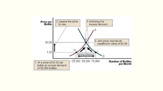
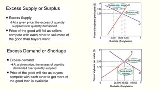
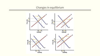
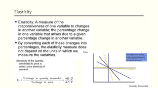
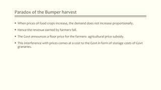
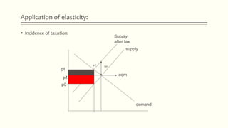
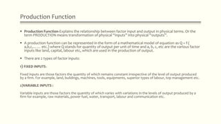
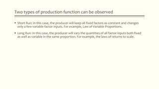
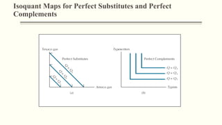
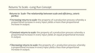
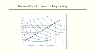
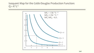
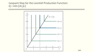
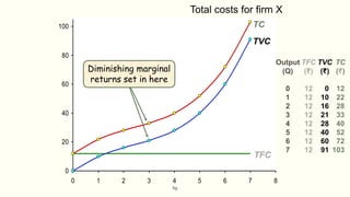
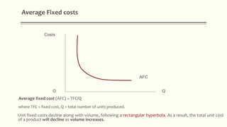
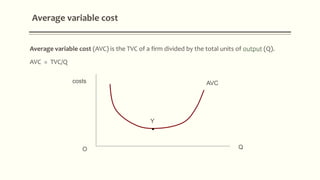
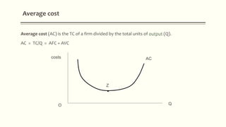
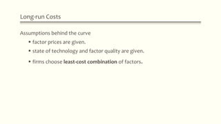
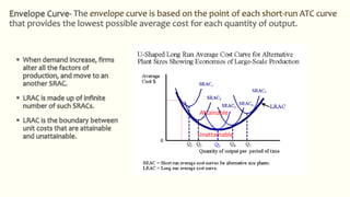
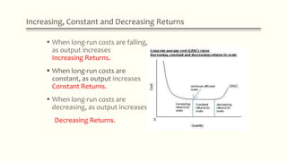
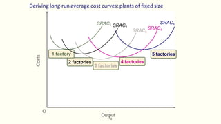
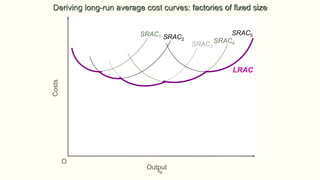
Microeconomics

MICROECONOMICS
BY:
CHHAVI DUDEJA
Economics is all about making choices in the presence of scarcity.

DIFFERENCE BETWEEN MICROECONOMICS AND
MACROECONOMICS
 Micro- study of how households and firms make decisions and how they interact in
markets. It is the study of individuals.
Also called price theory because it is primarily concerned with the determination of prices of
individual commodities and factors.
 Macro- study of economy wide phenomena, including inflation, unemployment and
economic growth.
Economic problem arises due to 3 reasons,
1) Human wants are unlimited
2) Resources are limited
3) Resources have alternative uses, which makes them all the more scarce
Central problem of an economy,
1) What to produce and in what quantity?
2) How to produce?
3) For whom to produce?

Important Concepts
 Production Possibility Curve: curve which depicts all possible combination of 2 goods which
an economy can produce with available technology and full and efficient use of given
resources.
 Opportunity cost: Quantity of a commodity sacrifices to produce other commodity.
 Marginal Opportunity Cost: Additional quantity of a commodity sacrificed to produce the
other good’s additional unit
Rightward shift is due to increase in
resources in an economy, for instance
*availability of new equipment
*increase in skilled and unskilled labor
through population growth
*increase in natural resources or a new
alternate found
*new technology introduced
Leftward shift is due to decrease in
volume of resources, for instance
*depreciation of machinery
*saturation of natural resources
*non-availability of equipment
*technology becomes obsolete

 Market Economy/Capitalist Economy: one in which all economic activities are organizes
through the market. Price mechanism works in such economy. Prices are determined by
the forces of demand and supply.
((The consumer’s choice is reflected in price. Quantity is demanded by consumers.
Producer’s produce those goods whose prices are relatively high to earn profit. Producers
supply.))
 Centrally Planned Economy: one in which important activities are planned and decided by
the central Planning authority i.e. Govt.

Consumer Behavior and DEMAND
 Utility: the power/capacity of a commodity to satisfy human wants.
 Marginal Utility (MU): additional utility derived from consumption of an additional unit of a
commodity. MUn= TUn-TUn-1
 Total Utility (TU): sum of all the utilities derived from consuming certain number of units of
a particular commodity. TU=∑MU
LAW OF DIMNISHING MU: as we increase our consumption MU derived from each succcesive
unit falls.

Consumer’s Equilibrium
 Situation wherein consumer spends his given income on purchasing a commodity and
gains maximum satisfaction, having no urge to change.
 Equilibrium can be observed through 2 approaches: Utility and Indifference curves.
1) Utility approach: condition says MU in terms of money=Price of the commodity
Alternatively, MU of the product/MU of rupee=price
UTILITY SCHEDULE OF A
CONSUMER

2) Indifference Curves- curve which shows all the possible combinations of 2 goods that give
the same level of satisfaction to the consumer. While, an Indifference map shows a number
of indifference curves possible of those 2 commodities.

Demand
 Refers to the quantity of a commodity which a consumer is willing and able to purchase at
different prices at a time.
 A demand function is a behavior function for consumers.
Dn=f(Price, price of related goods, income, tastes and preferences)
 Factors that affect demand are:
1) Price of the commodity- higher the price, lesser will be the demand
2) Price of related goods- if the related good is a SUBSITITUTE then if price of the good
increases, people will demand the substitute as it is now cheaper. If the related good is a
COMPLEMENTARY good then if price of the good decreases, people will buy both of them
(for instance if price of car falls, demand of petrol rises).
3) Income of the consumer- if the income increases they will demand more of normal
goods(rice, wheat) but if it decreases they will demand more of inferior goods(jowar, bajra).
4) Taste and preferences of the consumer

 Law of demand states that other things being constant, price and quantity demanded are
inversely related.
Here, assumptions are being made that price of related goods, income and tastes and
preferences being constant, there will be an inverse relation between price and demand. So
if price increases, demand will fall and vice-versa.

Supply
 Refers to quantity of a commodity which a producer is willing to sell at a particular price and time.
 A supply function is a behavior function for suppliers.
Sx=f(Px,T,Pi,Pr..)
 Factors that affect supply:
1) Price of the commodity: more the price, more the supplier would be willing to supply as the profit
margin increases. DIRECT RELATION.
2) Technology- advancement would reduce the cost of production and increase the supply.
3) Change in price of inputs- if factors of production increase, cost of production increases which leads to
fall in profit margin and hence suppliers would not like to produce/ supply.
4) Taxation policy/excide duty- if taxes are imposed on production or sales then cost increases and supply
falls.
5) Price of related goods- if price increases of a related good then the supplier would start producing more
of that commodity.

 Law of supply states that other things(factors) being constant, price and supply are
directly related.

Elasticity=(Percentage change in demand or supply / Percentage change in price)*100
=(Change in DD or SS/ Initial DD or SS) / (Change in Price/Initial price)
=(∆Q/Q) / (∆P/P)
=(P/Q) / (∆Q/∆P)

Determinants of Elasticity
 Number and closeness of substitutes –
the greater the number of substitutes,
the more elastic
 The proportion of income taken up by the product – the smaller the proportion the more
inelastic
 Price of the product- lower the price, lower the elasticity
 Luxury or Necessity - for example,
addictive drugs
 Time period – the longer the time under consideration the more elastic a good is likely to be

Cross-Price Elasticity
 Cross-price elasticity: A measure of the responsiveness of the demand for a
good to changes in the price of a related good; the percentage change in the
quantity demanded of one good divided by the percentage change in the
price of a related good.
 The cross-price elasticity is positive whenever goods are substitutes.
 The cross-price elasticity is negative whenever goods are complements.
How quantity of one good changes as price of another good increases
,
%change in quantity demanded
%change in price of another good
/
/
o
o
Q P
o o o
Q Q Q P
E
P P P Q
 
 
 

Income Elasticity
 Income elasticity: A measure of the responsiveness of the demand for a good
to changes in consumer income; the percentage change in quantity
demanded divided by the percentage change in income.
 The income elasticity is positive whenever the good is a normal good.
 The income elasticity is negative whenever the good is an inferior good.
% change in quantity demanded
% change in income
/
/
IE
Q Q Q I
Y Y Y Q

 
 
 

Factors affecting Income elasticity:
 Nature of the good:
 inferior goods have negative income elasticity
 Normal goods have positive income elasticity
 Luxury goods have income elasticity greater than one
 Necessary goods have income elasticity less than one

Elasticity and Total Revenue
 If demand is elastic, an increase (decrease) in price will lead to a decrease (increase) in
total revenue.
 If demand is inelastic, an increase (decrease) in price will lead to an increase (decrease) in
total revenue.
 Total revenue is maximized at the point where demand is unitary elastic.
price revenue elasticity
Increases increases E< 1
increases decreases E>1
decreases decreases E<1
decreases increases E>1
Increases/
decreases
constant E=1

Elasticity of Supply
 Price Elasticity of Supply:
 The responsiveness of supply to changes
in price
 If es is inelastic (<1)- it will be difficult for suppliers to react
swiftly to changes in price
 If es is elastic(>1) – supply can react quickly to changes in price
es =
% Δ Quantity Supplied____________________
% Δ Price

Paradox of the Bumper harvest
 When prices of food crops increase, the demand does not increase proportionally.
 Hence the revenue earned by farmers fall.
 The Govt announces a floor price for the farmers- agricultural price subsidy.
 This interference with prices comes at a cost to the Govt in form of storage costs of Govt
granaries.

Application of elasticity:
 Incidence of taxation:
Supply
after tax
supply
demand
taxe1
eqm
pt
p1
p0

Production Function
 Production Function-Explains the relationship between factor input and output in physical terms. Or the
term PRODUCTION means transformation of physical “inputs” into physical “outputs”.
 A production function can be represented in the form of a mathematical model of equation as Q = f (
a,b,c,…… etc.) where Q stands for quantity of output per unit of time and a, b, c, etc are the various factor
inputs like land, capital, labour etc, which are used in the production of output.
 There are 2 types of factor inputs:
1) FIXED INPUTS :
Fixed inputs are those factors the quantity of which remains constant irrespective of the level of output produced
by a firm. For example, land, buildings, machines, tools, equipments, superior types of labour, top management etc.
2)VARIABLE INPUTS :
Variable inputs are those factors the quantity of which varies with variations in the levels of output produced by a
firm for example, raw materials, power fuel, water, transport, labour and communication etc.

Two types of production function can be observed
 Short Run: In this case, the producer will keep all fixed factors as constant and changes
only a few variable factor inputs. For example, Law of Variable Proportions.
 Long Run: In this case, the producer will vary the quantities of all factor inputs both fixed
as well as variable in the same proportion. For example, the laws of returns to scale.

The law of Variable Proportions
 In the short-run -
the level of production can be changed by changing the factor proportions.
This law examines the production function with on factor variable, keeping the other factors
quantities fixed.
The law explains the short-run production function.
When the quantity of one input is varied, keeping other
inputs constant, the proportion between factors changes.
When the proportion of variable factors
increases, the total output does not always increase in the
same proportion, but in varying proportion.

 Only one factor is variable while others are held constant.
 All units of the variable factor are homogeneous.
 There is no change in Technology.
 It is possible to vary the proportions in which different inputs are combined.
 The products are measured in physical units, i.e., in quintals, tonnes etc.
Assumptions of the Law

 Total Product or Output (TP)- It refers to the total volume of goods produced during a
specified period of time. Total product (TP)can be raised only by increasing the quantity of
variable factors employed in production.
 Average Product (AP)- Average product can be known by dividing total product by the
total number of units of the variable factor.
APn=TPn/Q
 Marginal Product or Output (MP)- It is output derived from the employment of an
additional unit of variable factor unit. The rate at which total product increases is known as
marginal product.
MPn= TPn-TPn-1
Relationship between AP and MP
*When AP rises as a result of an increase in the quantity of variable input, MP is more then the average
product.
*When AP are maximum then MP is equal to AP. The MP curve cuts the AP curve at its maximum.
*When AP falls as a result of decrease in quantity of variable input, MP is less than the AP.

PRODUCTION SCHEDULE
QUANTITY OF
LABOUR
TOTAL
PRODUCT (TP)
AVERAGE
PRODUCT (AP)
MARGINAL
PRODUCT (MP)
1 2 2 2
2 6 3 4
3 12 4 6
4 16 4 4
5 18 3.6 2
6 18 3 0
7 14 2 -4
8 8 1 -6
Fixed Factor- Machinery
Variable Factor- Labour

Stage 1- THE LAW ON INCREASING RETURNS.
 TP increases at an increasing rate and both MP and AP also increase.
When production starts and we employ Variable factor over Fixed factor it leads
to optimum utilization of resources as there is division of labor and
specialization. In this stage the fixed factors are used to their fullest level. Also
here VF is less than FF capacity.
Stage 2- THE LAW OF DIMINSHING RETURNS.
 TP continues to increase at a diminishing rate, until it reaches it maximum point H.
 Both MP and AP continuously fall during this stage.
In this stage there is use of FF beyond its capacity because of which MP falls. There is a fall in quantity of fixed inputs per
VF. Here VF are more than FF capacity.
This stage is the ‘Real Stage of Production’ since TP is maximum here.
Stage 3- THE STATE OF NAGATIVE RETURNS
 TP declines.
 MP negative.
 AP is diminishing.
This happens due to overburdening of fixed factors

 A rational producer will never produce in stage 3, where MP is negative.
 A rational producer will also not produce in stage 1, where the MP of fixed factor is
negative.
 The producer producing in stage 1 will not be making best use of fixed factor and he will
not be utilizing fully the opportunity of increasing production by increasing quantity of
variable factor.
 A rational producer will produce in stage 2, where both MP and AP of variable factors are
diminishing.
CONCLUSION

Isoquant- the set of all input combinations that yield a
given level of output.
Marginal rate of technical substitution (MRTS): the rate at
which one input can be exchanged for another without
altering the total level of output.
Production In The Long Run

Part of an Isoquant Map for the Production Function
Part of an Isoquant Map for the Production Function The Marginal Rate of Technical Substitution
More is preferred
to less
Actual output
ΔQ0 =0 = Δ KMPK+ ΔLMPL
-ΔKMPK = ΔLMPL
|ΔK/ΔL| = MPL/MPK =MRTSL,K is the slope.

Isoquant Maps for Perfect Substitutes and Perfect
Complements

Returns To Scale –Long Run Concept
Returns to Scale--The relationship between scale and efficiency, ceteris
paribus
Increasing returns to scale: the property of a production process whereby a
proportional increase in every input yields a more than proportional
increase in output.
Constant returns to scale: the property of a production process whereby a
proportional increase in every input yields an equal proportional increase
in output.
Decreasing returns to scale: the property of a production process whereby
a proportional increase in every input yields a less than proportional
increase in output.

Returns to Scale Shown on the Isoquant Map

Isoquant Map for the Cobb-Douglas Production Function:
Q = K½L½
9-47
MPL= 1/2K1/2L-1/2
MPK=1/2K-1/2L1/2
MPL/MPK = K/L

Isoquant Map for the Leontief Production Function:
Q = min (2K,3L)
9-48

Explicit Cost
 The costs that have a money value like raw
materials, energy, rent, interest and wages
and have to be purchased from outside the
firm.(Accounting costs)
 (Accountant’s view)
Implicit cost
 The cost of using the firm’s own resources.
This is the earnings that a firm could have
had if it had employed its factors in another
use/hired/sold out.(Normal profit)
 (Economist’s view)
COSTS

Fixed cost does not change with the volume of production.
Cost- money expenditure incurred by a firm on producing the output
TFC
Q
costs
100
O
Cost of a firm (TC) is classified into two broad categories - Fixed cost (TFC) and Variable cost (TVC). i.e. TC = TFC + TVC
However, nothing is fixed in the long run.
Fixed costs- Fixed costs are expenses that does not change in proportion to the activity of a business. Fixed costs
include overheads (rent, insurance-premium, interests), and also direct costs such as payroll (particularly salaries).

Variable costs- Variable costs change in direct proportion to the activity of a business such as sales or
production volume. In retail, the cost of goods is almost entirely variable. In manufacturing, direct
material costs, wages, fuel costs are examples of variable costs.
For example, a manufacturing firm pays for raw materials. When activity is decreased, less raw
material is used, and so the spending for raw materials falls. When activity is increased, more raw
material is used and spending therefore rises.
Although tax usually varies with profit, which in turn varies with sales volume, it is not normally
considered a variable cost.

fig
0
20
40
60
80
100
0 1 2 3 4 5 6 7 8
TC
TVC
TFC
Diminishing marginal
returns set in here
Total costs for firm X
Output
(Q)
0
1
2
3
4
5
6
7
TFC
(₹)
12
12
12
12
12
12
12
12
TVC
(₹)
0
10
16
21
28
40
60
91
TC
(₹)
12
22
28
33
40
52
72
103

Average Fixed costs
Q
Costs
AFC
O
Average fixed cost (AFC) = TFC/Q
where TFC = fixed cost, Q = total number of units produced.
Unit fixed costs decline along with volume, following a rectangular hyperbola. As a result, the total unit cost
of a product will decline as volume increases.

Average variable cost
Average variable cost (AVC) is the TVC of a firm divided by the total units of output (Q).
AVC = TVC/Q
Q
costs
Y
AVC
O

Average cost
Average cost (AC) is the TC of a firm divided by the total units of output (Q).
AC = TC/Q = AFC + AVC
Q
costs
Z
AC
O

Marginal Cost
The additional cost incurred to produce one additional unit of output is called the Marginal Cost
(MC).
MC = dC/dQ
The marginal cost curve is U-shaped. Marginal cost is relatively high at small quantities of output -
then as production increases, it declines - then reaches a minimum value - then rises.
This shape of the marginal cost curve is directly attributable to increasing, then decreasing
marginal returns (the law of diminishing marginal returns).

figOutput (Q)
Costs(£)
MC
x
Diminishing marginal
returns set in here
Marginal costs

Numerical Example
Q TFC TVC TC AFC AVC AC MC
0 100 0 100
1 100 20 120 100 20 120 20
2 100 37 137 50 18.5 68.5 17
3 100 52 152 33.33 17.33 50.67 15
4 100 80 180 25 20 45 28
5 100 120 220 20 24 44 40
6 100 165 265 16.67 27.5 44.17 45

figOutput (Q)
Costs(£)
AFC
AVC
MC
x
AC
z
y
Average and marginal costs

Long run cost curves
The Long run average cost (LRAC or LAC) curve illustrates - for a given quantity of production - the
average cost per unit which a firm faces in the long run (i.e. when no factors of production is fixed).
 LRAC curve is derived from a series of short run average cost curves.
 It is also called the ‘Envelope curve' since it envelops all the short run average cost curve.
 The curve is created as an envelope of an infinite number of short-run average total cost curves.
The LRAC curve is U-shaped, reflecting economies of scale when it is negatively-sloped and
diseconomies of scale when it is positively sloped.
In perfect competition, the LRAC curve is flat at the point of equilibrium – in this stage the firm is
enjoying constant returns to scale.
In some industries, the LRAC is L-shaped, and economies of scale increase indefinitely. This means
that the largest firm tends to have a cost advantage, and the industry tends naturally to become a
monopoly, and hence is called a natural monopoly. Natural monopolies tend to exist in industries
with high capital costs in relation to variable costs, such as water supply and electricity supply.

fig
Long-run average cost curves
OutputO
Costs
LRAC
Economies of Scale

fig
OutputO
Costs LRAC
Diseconomies of Scale
long-run average cost curves

fig
OutputO
Costs
LRAC
Constant costs
long-run average cost curves

Long-run Costs
 Long-run average costs
 assumptions behind the curve
 factor prices are give
 state of technology and factor quality are given
 firms choose least-cost combination of factors

fig
OutputO
Costs
LRACEconomies
of scale
Constant
costs
Diseconomies
of scale
A typical long-run average cost curve

Long-run Costs
 Long-run average costs
 assumptions behind the curve
 factor prices are give
 state of technology and factor quality are given
 firms choose least-cost combination of factors
 shape of the LRAC curve
 a typical LRAC curve
 long-run average and marginal cost curves

fig
Long-run average and marginal costs
OutputO
Costs
LRAC
LRMC
Economies of Scale

fig
OutputO
Costs LRAC
LRMC
Diseconomies of Scale

fig
OutputO
Costs
LRAC = LRMC
Constant costs

fig
OutputO
Costs
LRMC
LRAC
Initial economies of scale,
then diseconomies of scale

Long-run Costs
Assumptions behind the curve
 factor prices are given.
 state of technology and factor quality are given.
 firms choose least-cost combination of factors.

Increasing, Constant and Decreasing Returns
 When long-run costs are falling,
as output increases
Increasing Returns.
 When long-run costs are
constant, as output increases
Constant Returns.
 When long-run costs are
decreasing, as output increases
Decreasing Returns.

fig
Deriving long-run average cost curves: plants of fixed size
SRAC3
Costs
Output
O
SRAC4
SRAC5
5 factories
4 factories
3 factories
2 factories
1 factory
SRAC1 SRAC2

fig
SRAC1
SRAC3
SRAC2 SRAC4
SRAC5
LRAC
Costs
Output
O
Deriving long-run average cost curves: factories of fixed size

fig
Deriving a long-run average cost curve: choice of factory size
Costs
Output
O
Examples of short-run
average cost curves

fig
LRAC
Costs
Output
O
Deriving a long-run average cost curve: choice of factory size

Revenue
Measurement of Revenue
Total
Revenue(TR)
Average
Revenue(AR)
Marginal
Revenue(MR)
Total Revenue- total amount of money realized by selling the total output.
TR=P*Q
TR=∑MR
TR=AR*Q
Average Revenue- revenue per unit sold.
AR=TR/Q
=(P*Q)/Q
=Price
Marginal Revenue- additional revenue generated by selling an additional unit of a product.
MRn=TRn-TRn-1

Total Revenue and Output
 TR when price does not change.(Horizontal demand
curve)
 The firm does not have to lower the price to sell
more output.
 If PED=Perfectly Elastic DD, then
 P=AR=MR=D
 TR curve is upward sloping.

Total Revenue and Output
 TR when price change as output increase.(downward sloping demand curve)
 Firm has to lower price to sell more.
 PED falls as output increases.

Relationship between TR, AR, MR and PED.
 TR rises at first but will eventually falls as output
increases.
When PED is elastic, to increase revenue, lower the
price.
When PED is inelastic, to increase revenue, raise the
price.
When PED is unity, to increase revenue, leave the
price unchanged.

Profit Theory
Generally, Profit =TR-TC.
But for an economist, Profit= TR-Economic Cost(Explicit + Implicit Cost)
For instance, there are 3 firms, A,B,C
Firm A: TR>TC Abnormal Profit
Firm B: TR=TC Normal Profit
Firm C: TR<TC Loss
Firm A Firm B Firm C
Total Revenue 200 000 200 000 200 000
TFC 40 000 40 000 40 000
TVC 80 000 100 000 120 000
Implicit Cost 60 000 60 000 60 000
Total Cost 180 000 200 000 220 000

Firm A Firm B Firm C
TR 80 000 120 000 150 000
TFC(including opp.cost) 100 000 100 000 100 000
TVC 100 000 120 000 140 000
TC 200 000 220 000 240 000
Loss 120 000 100 000 90 000
Firm A: Loss = FC+20 000 VC
Firm B: Loss = FC
Firm C: Loss = <FC
Whether to produce or not?

Shut down Price
 At price P, firm is able to cover variable cost in
the short run.
 Shut down price is P.
 P=AVC
 Below this price, firm will shut down in the
short-run.
P1 =ATC
P=AVC

Break-even price
P1 =ATC
P=AVC
•The break even price is the price
at which a firm is able to make
normal profit in the long run.
•At this price the firm is able to
cover all of its cost.
•P=ATC
•Below price P1, firm will shut
down in the long run.

Profit Maximizing level of output
 The level of output that the firm achieves the
maximum profit.
 MC=MR
 M is the profit minimization output.
 M1 is the profit maximization output.
 MC curve cuts the MR curve from below.
 Till M, MC>MR
 Between M and M1, MC<MR
 Beyond M1, MC>MR

Profit Maximizing level of output
 Normal Demand Curve situation:
 Profit maximization output is the level of
output where MC cuts MR from below.
 Price is Pm, because consumers are
willing to pay this much.

Measuring abnormal profit
 MC curve cuts the AC curve at the
lowest point.
 Profit per unit is AR-AC.
 Total abnormal profit= ab x OQn

Abnormal Profit, Normal Profit & Loss
 Whether a firm earns abnormal
profit, normal profit or loss is
depended on the position of the AC
curves.
 If average cost is: AC1, abnormal
profit
 AC*, normal profit
 AC2,loss.
AR>AC
AR=A
C
AR<AC

Microeconomics

More Related Content

What's hot

Similar to Microeconomics

Recently uploaded

Microeconomics