This document provides an introduction to queueing theory. It defines key terms like queues, congestion, and queueing systems. Queueing theory is applied in many fields like telecommunications, healthcare, and manufacturing to model waiting lines and predict performance. Little's Law relates the average number of tasks in a system to the arrival rate and average time spent in the system. The document gives examples of applying queueing theory to model retail checkout lines and computer networks. It outlines the key characteristics used to describe queueing systems, such as arrival and service processes, and the Kendall notation used to specify queueing models.

1. Introduction to
Queueing Theory
Presented by
Ms.S.R.Vidhya
Assistant Professor of Mathematics,
Bon Secours College for Women, Thanjavur.

2. 2
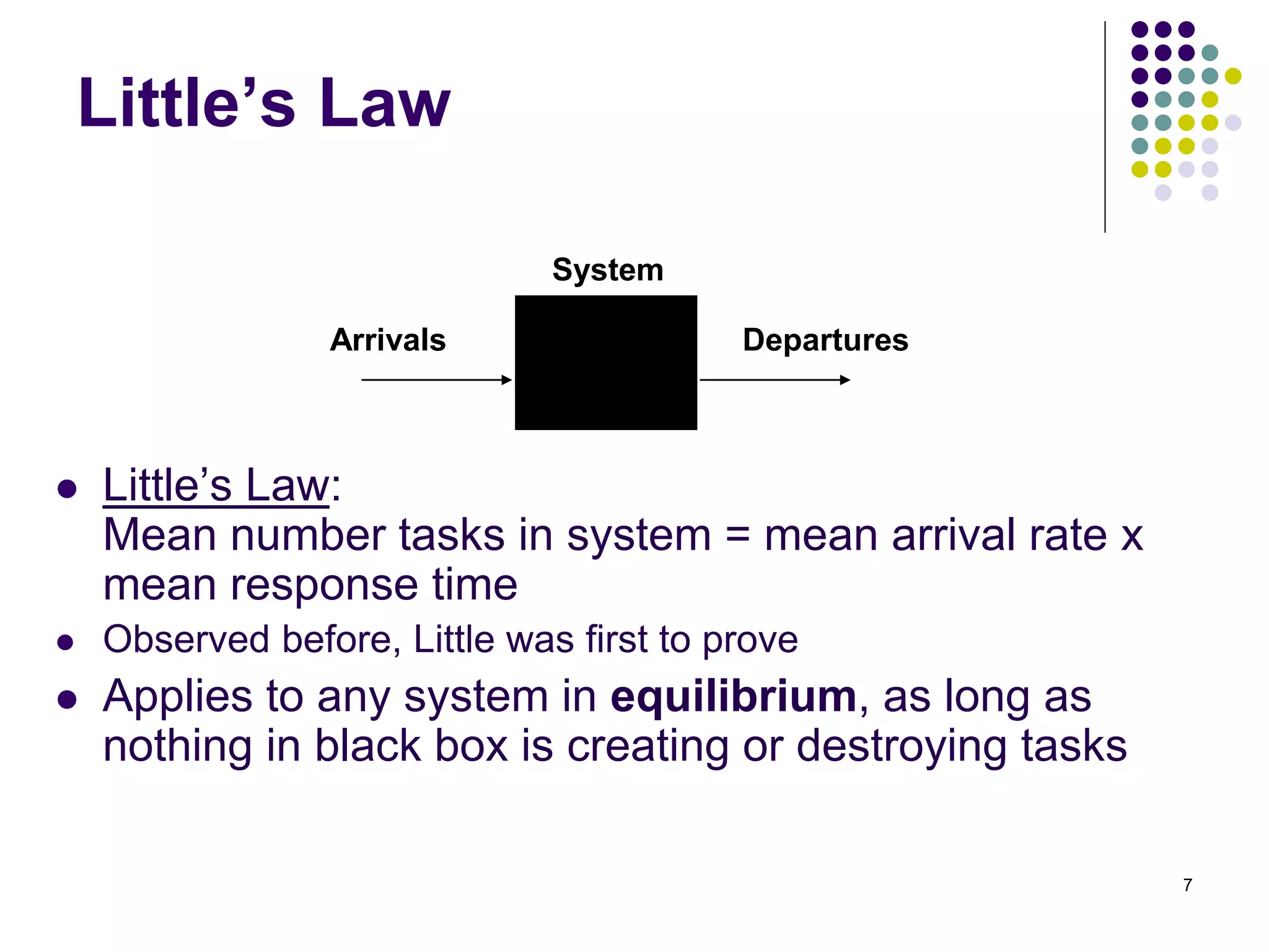
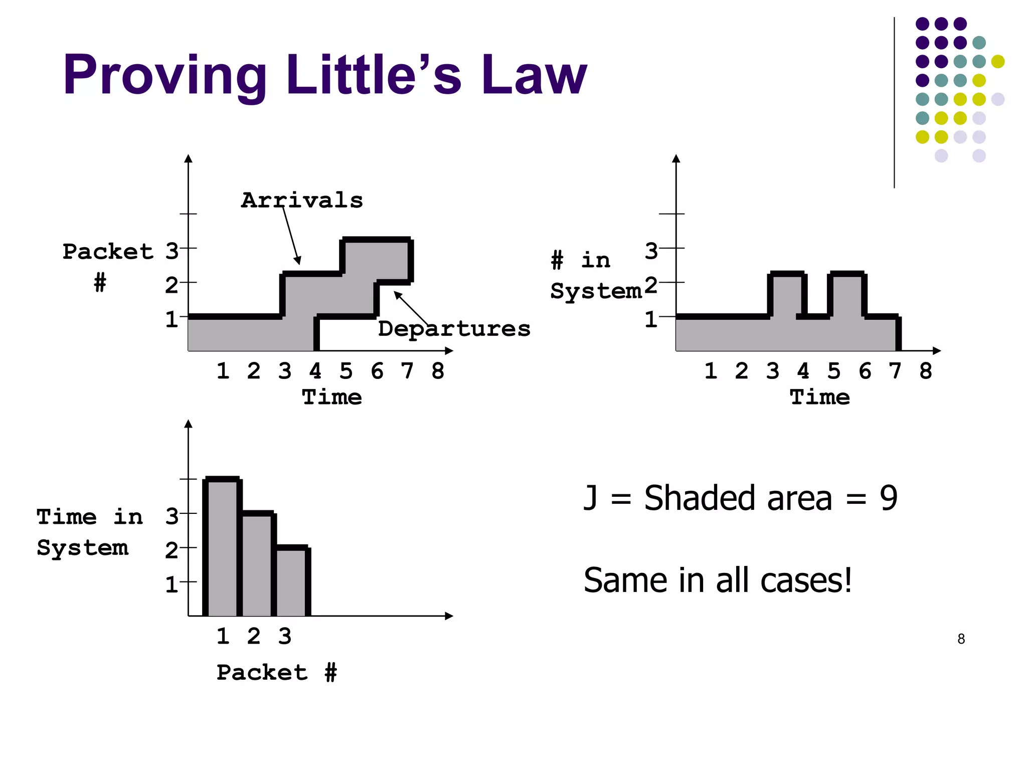
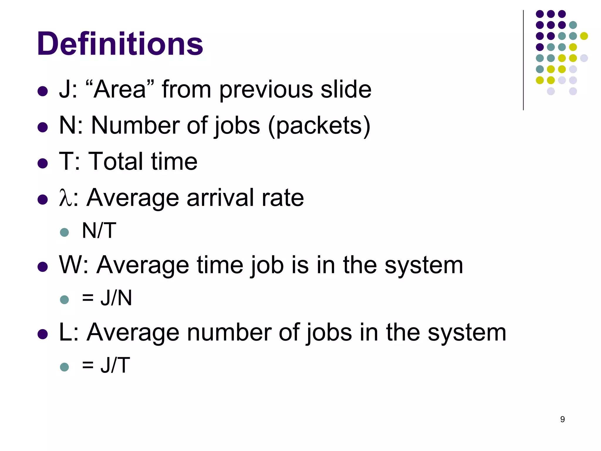
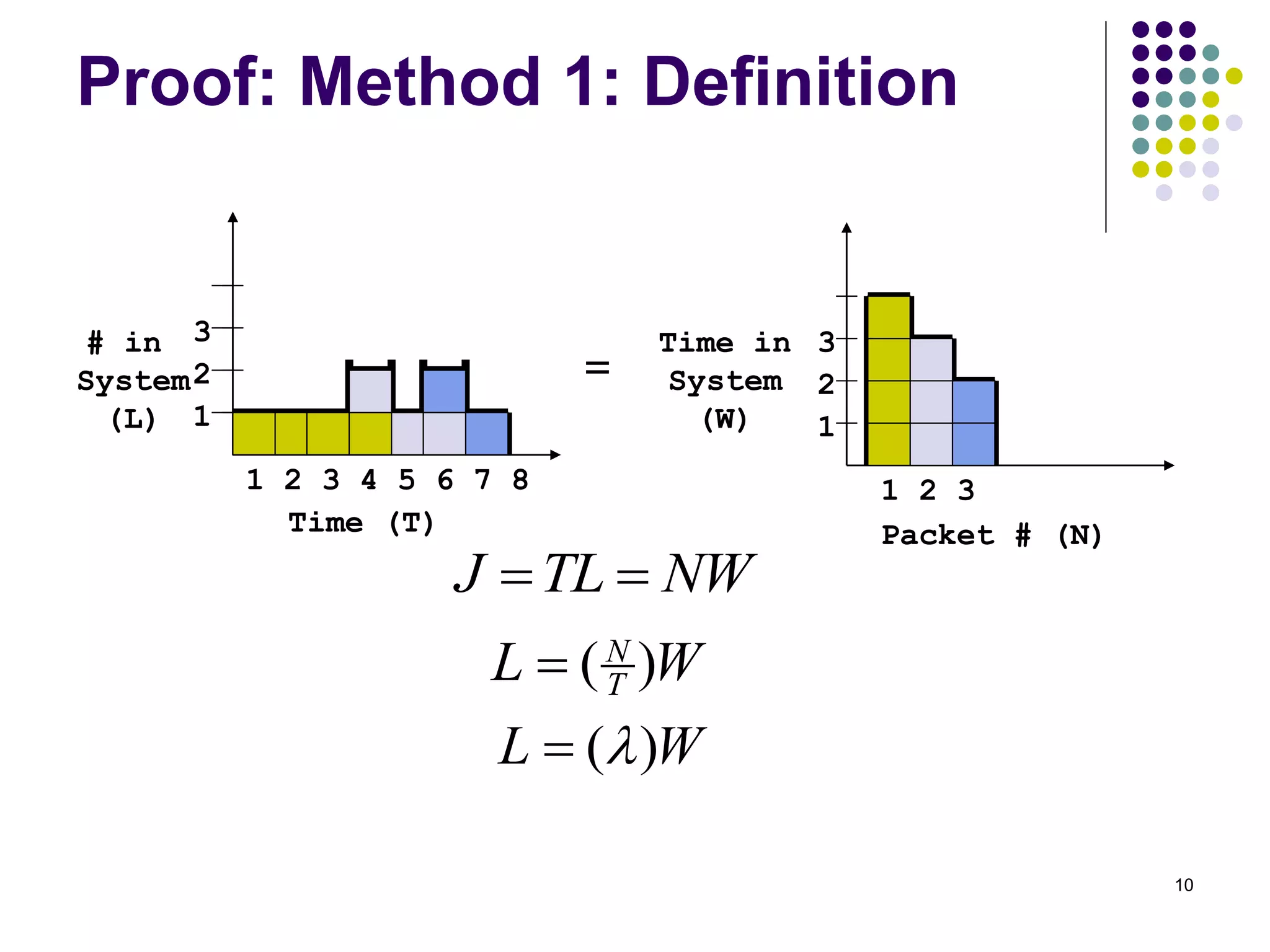
Queueing theory definitions
 (Bose) “the basic phenomenon of queueing arises
whenever a shared facility needs to be accessed
for service by a large number of jobs or
customers.”
 (Wolff) “The primary tool for studying these
problems [of congestions] is known as queueing
theory.”
 (Kleinrock) “We study the phenomena of
standing, waiting, and serving, and we call this
study Queueing Theory." "Any system in which
arrivals place demands upon a finite capacity
resource may be termed a queueing system.”
 (Mathworld) “The study of the waiting times,
lengths, and other properties of queues.”

3. 3
Applications of Queuing Theory
 Telecommunications
 Traffic control
 Determining the sequence of computer
operations
 Predicting computer performance
 Health services (ex. control of hospital
bed assignments)
 Airport traffic, airline ticket sales
 Layout of manufacturing systems.

4. 4
Example application of
Queueing theory
 In many retail stores and banks
multiple line/multiple checkout system  a queuing
system where customers wait for the next available
cashier
We can prove using queuing theory that : throughput
improves increases when queues are used instead
of separate lines

5. 5
Example Application of
Queueing Theory

6. 6
Queueing Theory for studying
networks
 View network as collections of queues
 FIFO data-structures
 Queuing theory provides probabilistic
analysis of these queues
 Examples:
 Average length
 Average waiting time
 Probability queue is at a certain length
 Probability a packet will be lost

7. 7
Little’s Law
 Little’s Law:
Mean number tasks in system = mean arrival rate x
mean response time
 Observed before, Little was first to prove
 Applies to any system in equilibrium, as long as
nothing in black box is creating or destroying tasks
Arrivals Departures
System

8. 8
Proving Little’s Law
J = Shaded area = 9
Same in all cases!
1 2 3 4 5 6 7 8
Packet
#
Time
1
2
3
1 2 3 4 5 6 7 8
# in
System
1
2
3
Time
1 2 3
Time in
System
Packet #
1
2
3
Arrivals
Departures

9. 9
Definitions
 J: “Area” from previous slide
 N: Number of jobs (packets)
 T: Total time
 l: Average arrival rate
 N/T
 W: Average time job is in the system
 = J/N
 L: Average number of jobs in the system
 = J/T

10. 10
1 2 3 4 5 6 7 8
# in
System
(L) 1
2
3
Proof: Method 1: Definition
Time (T)
1 2 3
Time in
System
(W)
Packet # (N)
1
2
3
=
W
L T
N
)
(

NW
TL
J 

W
L )
(l


11. 11
Proof: Method 2: Substitution
W
L T
N
)
(

W
L )
(l

)
)(
( N
J
T
N
T
J

T
J
T
J
 Tautology

12. 12
Model Queueing System
Server System
Queuing System
Queue Server
Queuing System
 Use Queuing models to
 Describe the behavior of queuing systems
 Evaluate system performance

13. 13
Characteristics of Queueing
Systems
 Arrival Process
 The distribution that determines how the tasks
arrives in the system.
 Service Process
 The distribution that determines the task
processing time
 Number of Servers
 Total number of servers available to process the
tasks

14. 14
Kendall Notation 1/2/3(/4/5/6)
 Six parameters in shorthand
 First three typically used, unless specified
1. Arrival Distribution
2. Service Distribution
3. Number of servers
4. Total Capacity (infinite if not specified)
5. Population Size (infinite)
6. Service Discipline (FCFS/FIFO)