CS352 - Introduction
to Queuing Theory
Rutgers University
CS352 Fall,2005 2
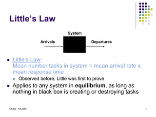
Queuing theory definitions
 (Bose) “the basic phenomenon of queueing arises
whenever a shared facility needs to be accessed for
service by a large number of jobs or customers.”
 (Wolff) “The primary tool for studying these
problems [of congestions] is known as queueing
theory.”
 (Kleinrock) “We study the phenomena of standing,
waiting, and serving, and we call this study
Queueing Theory." "Any system in which arrivals
place demands upon a finite capacity resource may
be termed a queueing system.”
 (Mathworld) “The study of the waiting times, lengths,
and other properties of queues.”
http://www2.uwindsor.ca/~hlynka/queue.html
CS352 Fall,2005 3
Applications of Queuing
Theory
 Telecommunications
 Traffic control
 Determining the sequence of computer
operations
 Predicting computer performance
 Health services (eg. control of hospital bed
assignments)
 Airport traffic, airline ticket sales
 Layout of manufacturing systems.
http://www2.uwindsor.ca/~hlynka/queue.html
CS352 Fall,2005 4
Example application of
queuing theory
 In many retail stores and banks
 multiple line/multiple checkout system  a
queuing system where customers wait for the next
available cashier
 We can prove using queuing theory that :
throughput improves increases when queues are
used instead of separate lines
http://www.andrews.edu/~calkins/math/webtexts/prod10.htm#QT
CS352 Fall,2005 5
Example application of
queuing theory
http://www.bsbpa.umkc.edu/classes/ashley/Chaptr14/sld006.htm
CS352 Fall,2005 6
Queuing theory for studying
networks
 View network as collections of queues
 FIFO data-structures
 Queuing theory provides probabilistic
analysis of these queues
 Examples:
 Average length
 Average waiting time
 Probability queue is at a certain length
 Probability a packet will be lost
CS352 Fall,2005 7
Little’s Law
 Little’s Law:
Mean number tasks in system = mean arrival rate x
mean response time
 Observed before, Little was first to prove
 Applies to any system in equilibrium, as long as
nothing in black box is creating or destroying tasks
Arrivals Departures
System
CS352 Fall,2005 8
Proving Little’s Law
J = Shaded area = 9
Same in all cases!
1 2 3 4 5 6 7 8
Packet
#
Time
1
2
3
1 2 3 4 5 6 7 8
# in
System
1
2
3
Time
1 2 3
Time in
System
Packet #
1
2
3
Arrivals
Departures
CS352 Fall,2005 9
Definitions
 J: “Area” from previous slide
 N: Number of jobs (packets)
 T: Total time
 l: Average arrival rate
 N/T
 W: Average time job is in the system
 = J/N
 L: Average number of jobs in the system
 = J/T
CS352 Fall,2005 10
1 2 3 4 5 6 7 8
# in
System
(L) 1
2
3
Proof: Method 1: Definition
Time (T)
1 2 3
Time in
System
(W)
Packet # (N)
1
2
3
=
W
L T
N
)
(

NW
TL
J 

W
L )
(l

CS352 Fall,2005 11
Proof: Method 2: Substitution
W
L T
N
)
(

W
L )
(l

)
)(
( N
J
T
N
T
J

T
J
T
J
 Tautology
CS352 Fall,2005 12
Model Queuing System
Server System
Queuing System
Queue Server
Queuing System
 Use Queuing models to
 Describe the behavior of queuing systems
 Evaluate system performance
CS352 Fall,2005 13
Characteristics of queuing
systems
 Arrival Process
 The distribution that determines how the tasks
arrives in the system.
 Service Process
 The distribution that determines the task
processing time
 Number of Servers
 Total number of servers available to process the
tasks
CS352 Fall,2005 14
Kendall Notation 1/2/3(/4/5/6)
 Six parameters in shorthand
 First three typically used, unless specified
1. Arrival Distribution
2. Service Distribution
3. Number of servers
4. Total Capacity (infinite if not specified)
5. Population Size (infinite)
6. Service Discipline (FCFS/FIFO)
Interesting, right?
This is just a sneak preview of the full presentation. We hope
you like it! To see the rest of it, just click here to view it in full
on PowerShow.com. Then, if you’d like, you can also log in to
PowerShow.com to download the entire presentation for free.

queuing-theory.2858801.powerpoint.pptx

  • 1.
    CS352 - Introduction toQueuing Theory Rutgers University
  • 2.
    CS352 Fall,2005 2 Queuingtheory definitions  (Bose) “the basic phenomenon of queueing arises whenever a shared facility needs to be accessed for service by a large number of jobs or customers.”  (Wolff) “The primary tool for studying these problems [of congestions] is known as queueing theory.”  (Kleinrock) “We study the phenomena of standing, waiting, and serving, and we call this study Queueing Theory." "Any system in which arrivals place demands upon a finite capacity resource may be termed a queueing system.”  (Mathworld) “The study of the waiting times, lengths, and other properties of queues.” http://www2.uwindsor.ca/~hlynka/queue.html
  • 3.
    CS352 Fall,2005 3 Applicationsof Queuing Theory  Telecommunications  Traffic control  Determining the sequence of computer operations  Predicting computer performance  Health services (eg. control of hospital bed assignments)  Airport traffic, airline ticket sales  Layout of manufacturing systems. http://www2.uwindsor.ca/~hlynka/queue.html
  • 4.
    CS352 Fall,2005 4 Exampleapplication of queuing theory  In many retail stores and banks  multiple line/multiple checkout system  a queuing system where customers wait for the next available cashier  We can prove using queuing theory that : throughput improves increases when queues are used instead of separate lines http://www.andrews.edu/~calkins/math/webtexts/prod10.htm#QT
  • 5.
    CS352 Fall,2005 5 Exampleapplication of queuing theory http://www.bsbpa.umkc.edu/classes/ashley/Chaptr14/sld006.htm
  • 6.
    CS352 Fall,2005 6 Queuingtheory for studying networks  View network as collections of queues  FIFO data-structures  Queuing theory provides probabilistic analysis of these queues  Examples:  Average length  Average waiting time  Probability queue is at a certain length  Probability a packet will be lost
  • 7.
    CS352 Fall,2005 7 Little’sLaw  Little’s Law: Mean number tasks in system = mean arrival rate x mean response time  Observed before, Little was first to prove  Applies to any system in equilibrium, as long as nothing in black box is creating or destroying tasks Arrivals Departures System
  • 8.
    CS352 Fall,2005 8 ProvingLittle’s Law J = Shaded area = 9 Same in all cases! 1 2 3 4 5 6 7 8 Packet # Time 1 2 3 1 2 3 4 5 6 7 8 # in System 1 2 3 Time 1 2 3 Time in System Packet # 1 2 3 Arrivals Departures
  • 9.
    CS352 Fall,2005 9 Definitions J: “Area” from previous slide  N: Number of jobs (packets)  T: Total time  l: Average arrival rate  N/T  W: Average time job is in the system  = J/N  L: Average number of jobs in the system  = J/T
  • 10.
    CS352 Fall,2005 10 12 3 4 5 6 7 8 # in System (L) 1 2 3 Proof: Method 1: Definition Time (T) 1 2 3 Time in System (W) Packet # (N) 1 2 3 = W L T N ) (  NW TL J   W L ) (l 
  • 11.
    CS352 Fall,2005 11 Proof:Method 2: Substitution W L T N ) (  W L ) (l  ) )( ( N J T N T J  T J T J  Tautology
  • 12.
    CS352 Fall,2005 12 ModelQueuing System Server System Queuing System Queue Server Queuing System  Use Queuing models to  Describe the behavior of queuing systems  Evaluate system performance
  • 13.
    CS352 Fall,2005 13 Characteristicsof queuing systems  Arrival Process  The distribution that determines how the tasks arrives in the system.  Service Process  The distribution that determines the task processing time  Number of Servers  Total number of servers available to process the tasks
  • 14.
    CS352 Fall,2005 14 KendallNotation 1/2/3(/4/5/6)  Six parameters in shorthand  First three typically used, unless specified 1. Arrival Distribution 2. Service Distribution 3. Number of servers 4. Total Capacity (infinite if not specified) 5. Population Size (infinite) 6. Service Discipline (FCFS/FIFO)
  • 15.
    Interesting, right? This isjust a sneak preview of the full presentation. We hope you like it! To see the rest of it, just click here to view it in full on PowerShow.com. Then, if you’d like, you can also log in to PowerShow.com to download the entire presentation for free.