Queuing theory project

1. Queuing Theory and Its Application
• Presented by: Izharul Owadud
• Department of Mathematics, Arya Vidyapeeth
College
• Paper Code: MAT-HC-6086

2. Introduction
• • Study of queues and waiting lines
• • Helps balance service capacity and wait
times
• • Applications: hospitals, banks, traffic, etc.

3. History of Queuing Theory
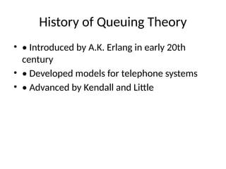
• • Introduced by A.K. Erlang in early 20th
century
• • Developed models for telephone systems
• • Advanced by Kendall and Little

4. Importance of Queuing Theory
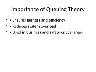
• • Ensures fairness and efficiency
• • Reduces system overload
• • Used in business and safety-critical areas

5. Basic Definitions
• • Customer, Server, Queue
• • λ = Arrival rate, µ = Service rate
• • ρ = Traffic intensity (λ/µ)

6. Components of a Queue System
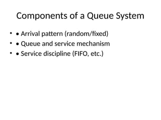
• • Arrival pattern (random/fixed)
• • Queue and service mechanism
• • Service discipline (FIFO, etc.)

7. Queue Disciplines
• • FIFO: First come, first served
• • FILO: Last in, first out
• • SIRO: Random service
• • Priority and processor sharing

8. Notations & Little’s Law
• • Key metrics: L, W, Lq, Wq
• • Little’s Law: L = λW
• • Helps in performance prediction

9. Kendall’s Notation
• • Format: A/B/m/K/n/D
• • Example: M/M/1 = Poisson arrivals,
exponential service, 1 server
• • Simplifies model classification

10. Queuing Models
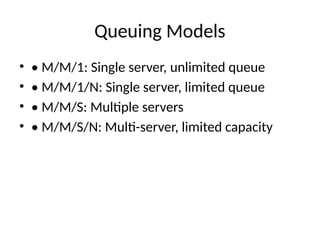
• • M/M/1: Single server, unlimited queue
• • M/M/1/N: Single server, limited queue
• • M/M/S: Multiple servers
• • M/M/S/N: Multi-server, limited capacity

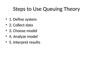
11. Steps to Use Queuing Theory
• 1. Define system
• 2. Collect data
• 3. Choose model
• 4. Analyze model
• 5. Interpret results

12. Case Study – Hang Out Restaurant
• • Location: Uzanbazar, Guwahati
• • 40 tables, 25 waiters
• • 800–1300 customers/day
• • Issue: High wait times

13. Analysis of Restaurant Queue
• • Model: M/M/1
• • λ = 3.22/min, µ = 3.24/min
• • ρ = 0.994 (high utilization)
• • Avg wait time: ~11 mins

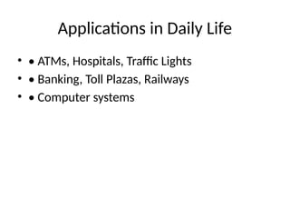
14. Applications in Daily Life
• • ATMs, Hospitals, Traffic Lights
• • Banking, Toll Plazas, Railways
• • Computer systems

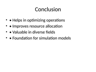
15. Conclusion
• • Helps in optimizing operations
• • Improves resource allocation
• • Valuable in diverse fields
• • Foundation for simulation models