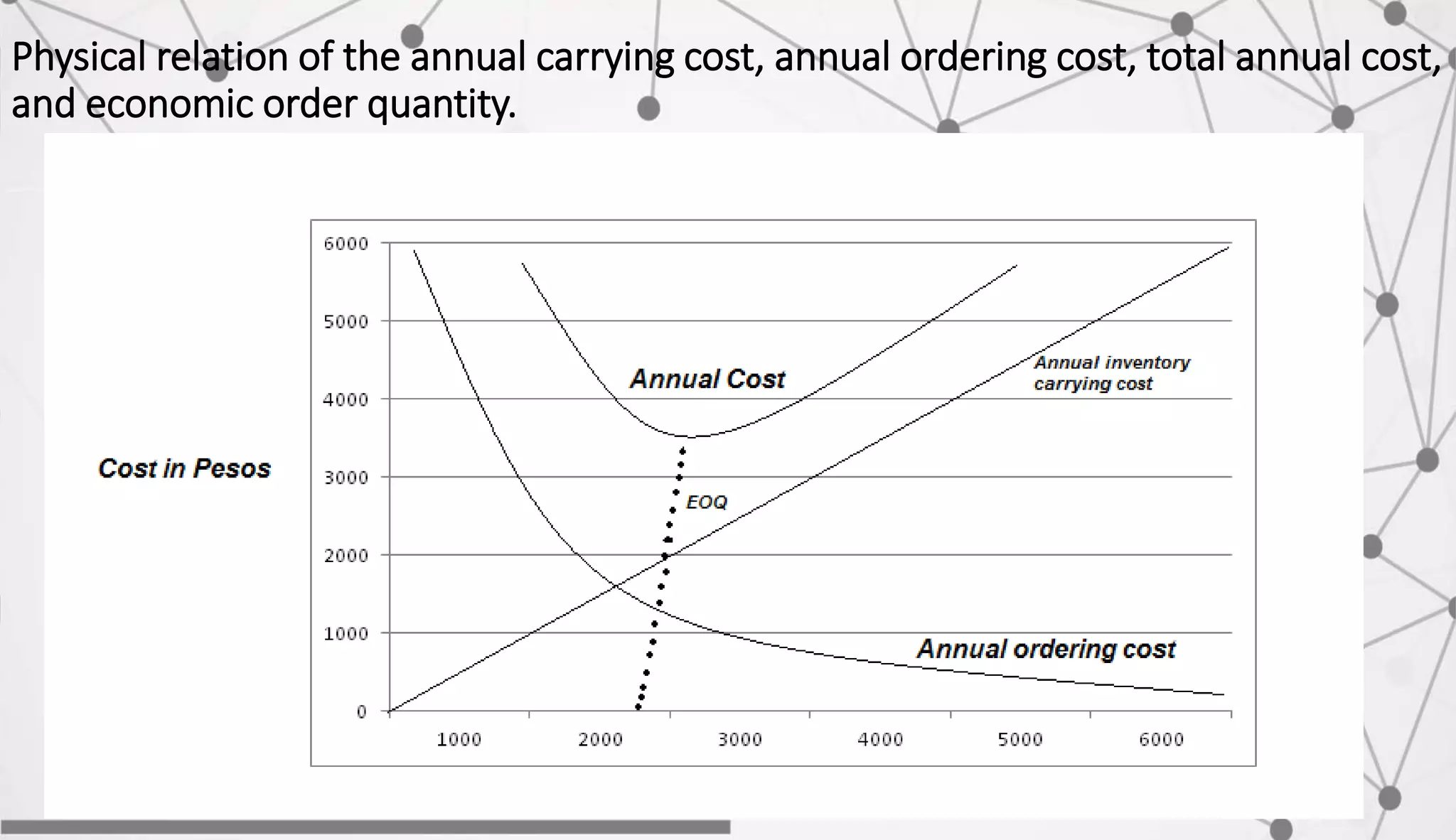
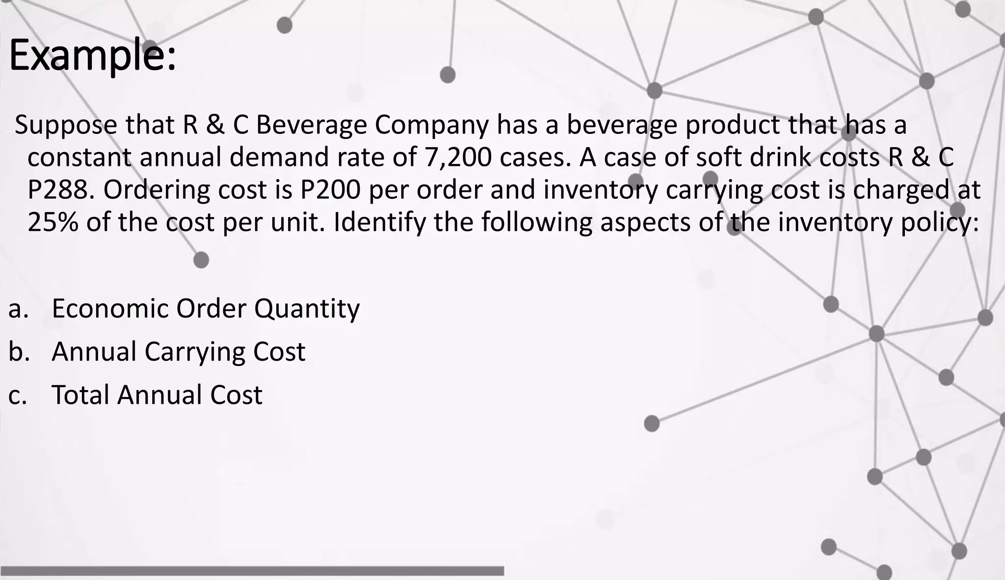
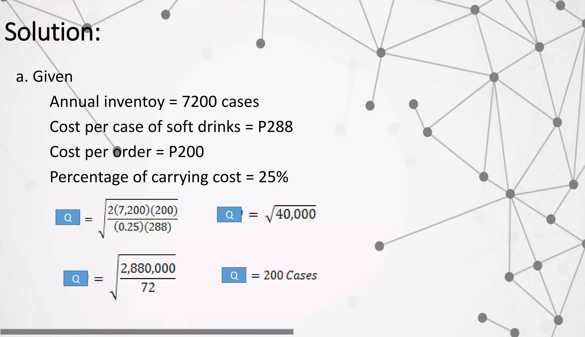
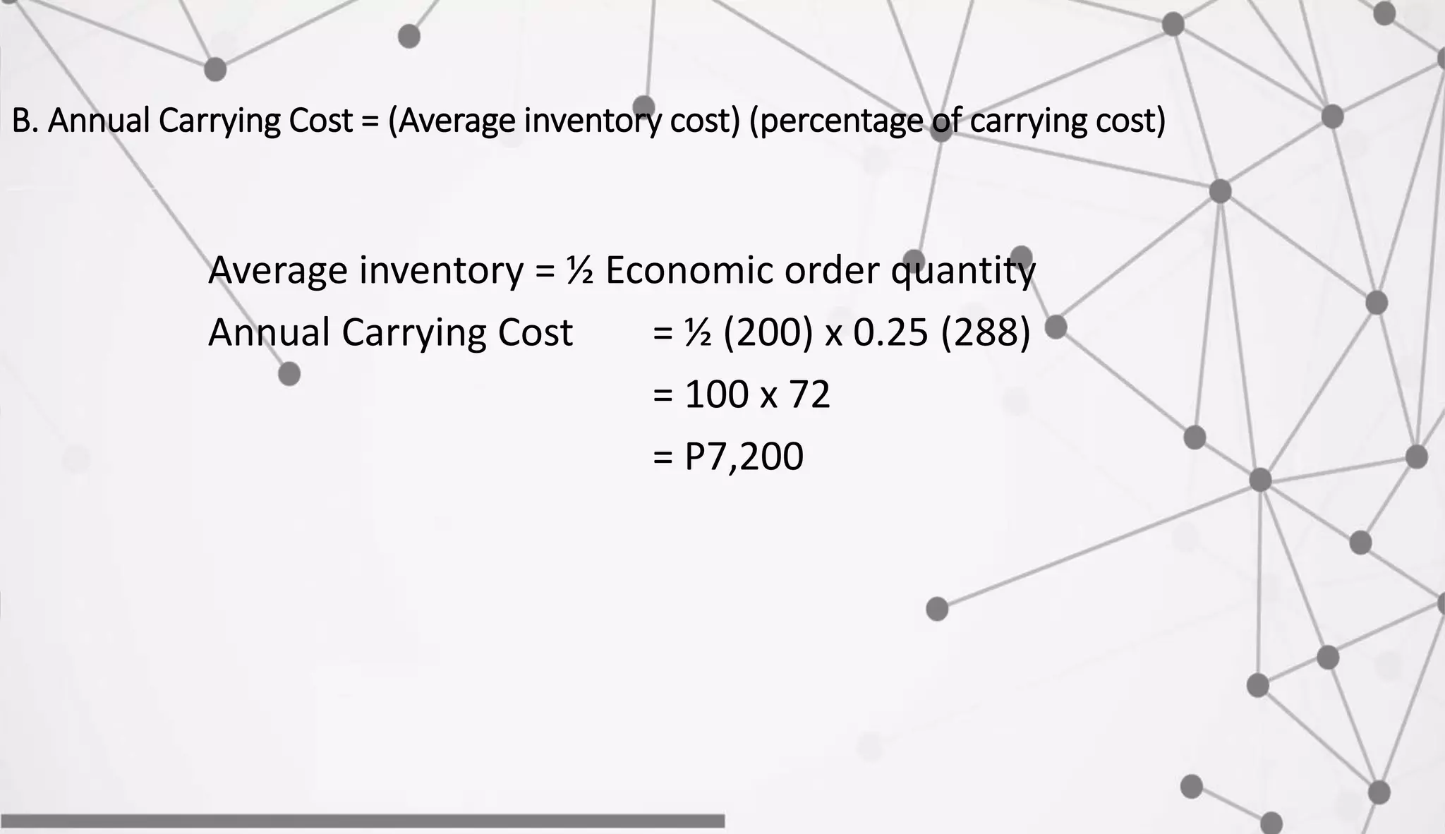
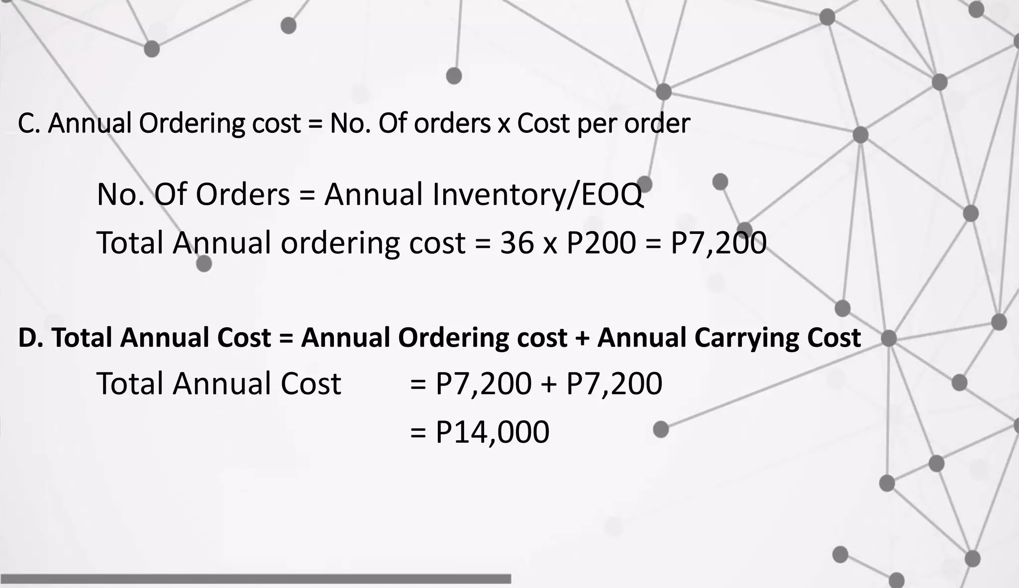
Chapter 5
Decision Theory
Mathematical Expectation or expected value
is the product of the probability for an event will occur and the
amount to be received upon such an occurrence.
The Concept of Probability
• It is more often that we are compelled to predict the outcome of
future events based on the repeated experiments of observation of
the same events under the same condition. The probability of
occurrence of the event(called success) and the probability of
occurrence (called failure) is equal to 1 or 100%.
What is PROBABILITY?
Probability
• is an event that ranges to 0 to 1, probability of success is 1 or 100%;
if the event cannot occur, is probability is 0.
Computation of mathematical
expectation or expected value
Let P represent the probability value and X represent the amount of many
mathematical expectation is computed as:
EV = P(X)
If the event has several possible outcome with probability
𝑃1, 𝑃2, 𝑃3, ……. 𝑃𝑛 and EV denotes a discrete variable.
𝐸𝑉 = 𝑃1(𝑋1) + 𝑃2(𝑋2) + 𝑃3 𝑋3 + … 𝑃𝑛(𝑋 𝑛)
Example 1:
A fair coin is tossed. If the coin lands heads, Mr. A will receive
Php. 6.00, and pay Php. 4.00 if it lands tails. Find 𝐸𝑉.
There is only 2 possible outcomes, heads or tails, the probability
of heads is
1
2
, and that of tails is also
1
2
, so
Let 𝑃1 = ℎ𝑒𝑎𝑑𝑠 and 𝑃2 = 𝑡𝑎𝑖𝑙𝑠
Given:
𝑃1 =
1
2
𝑋1 = 6
𝑃2 =
1
2
𝑋2 = 4
Computation:
𝐸𝑉 =
1
2
6 +
1
2
(−4)
𝐸𝑉 = 3 − 2
𝐸𝑉 = 𝑃ℎ𝑝1.00 (This means the game is fair for Mr. A)
What is DECISION MAKING UNDER
CERTAINTY?
Decision-making under certainty
The possible future conditions will actually happen when the
manager know which event will occur. The decision maker is to pick
the alternative with the best pay off for the known event. The best
alternative is the highest pay off if the pay offs are expressed in
profits. If the pay offs are expressed as costs, the best alternative is
the lowest pay off.
Example:
Which is the best alternative if the probability of small demand
is estimated to be 0.4 and the probability of large demand is
estimated to be 0.6?
Therefore: The large facility is the highest expected value which 612.
Possible Future
Demand
Alternative Low High Expected Value (EV)
Small Facility 300 370 𝟎. 𝟒 𝟑𝟎𝟎 + 𝟎. 𝟔 𝟑𝟕𝟎 = 𝟑𝟒𝟐
Large Facility 301 900 𝟎. 𝟒 𝟏𝟖𝟎 + 𝟎. 𝟔 𝟗𝟎𝟎 = 𝟔𝟏𝟐
What is DECISION MAKING UNDER
UNCERTAINTY?
Decision making under uncertainty
We assume the manager can list the possible events but cannot
estimate their probabilities. Perhaps the lack of prior experience
makes it difficult for the firm to estimate probabilities.
The following conditions will be used
in decision rules:
1. Maximin
2. Maximax
3. Laplace
4. Minimax Regret
Maximin – choose the alternative that is the “best of
the best.” This maximin approach is essentially a
pessimistic one because it takes into account the
worst possible outcome for each alternative.
Example: A. Maximin
Alternative Worst Payoff
Small facilitys 300
Large facility 180
Since P300.00 is the worst member, the pessimist would build a small
facility.
Maximax – choose the alternative that is the
“best of the worst.” The maximax approach
is an optimistic, “go for it” strategy that has
high expectations.
Example: B. Maximax
Alternative Best Payoff
Small facility 370
Large facility 900
Since P900,000 is the best member, the optimist would build a large
facility.
Laplace – choose the alternative with the best
“weighted payoff.” The Laplace approach treats
the states of nature as equally likely (equal
probability) to each event.
Example: C. Laplace
Alternative Weighted Payoff
Small facility 0.5(300) + 0.5(370) = 335
Large facility 0.5 (180) + 0.5(900) =
540
Since P540,000 is the best weighted payoff, the realist would build a
large facility.
Minimax Regret – choose the alternative
with the best “worst regret.” This approach
seeks to minimize the difference between
the given payoff and the best payoff for each
state of nature.
Example: Minimax Regret
To solve this problem, find the difference between a given payoff and the best payoff.
Let us consider, in the first column, the best payoff is 300, the remaining column must
be subtracted from 300.
Alternative REGRET Maximum Regret
Low Demand High Demand
Small Facility 300 – 300 = 0 900 – 370 = 530 530
Large Facility 300 – 180 = 120 900 – 900 = 0 120
Since the column on the right shows the worst regret for each alternative, pick a
large facility to minimize the maximum regret. The biggest regret is associated with
having only a small facility and high demand.
What is DECISION MAKING UNDER RISK?
Decision making under risk
The manager has less information than with decision-making under
certainty but more information than with decision-making under
uncertainty. A widely used approach under such circumstances is the
expected value. The expected value (EV) is the sum of the payoffs for
an alternative where each payoff is weighted by the probability for
the relevant state of mature.
Example:
Which is the best alternative if the probability of small demand is estimated
to be 0.4 and the probability of large demand is estimated to be
0.60(60%)?
Possible Future Demand
Alternative Low High Expected Value
Small Facility 300 370 0.4(300)+0.6(370) = 342
Large Facility 180 900 0.4(180)+0.6(900) = 612
Therefore: Large facility is the highest expected value which is 612.
What is a DECISION TREE?
Decision Tree
A decision tree is a schematic model of alternative available to
the decision make along with their possible consequences. A decision
tree is composed of a number of nodes that have branches
emanating from it. Two types of nodes are used in such a tree: a
square represent a decision point and a circle stands for a chance
event.
Two types of nodes
• Square represent a decision point
• Circle stands for a chance event
After the tree has been drawn, analyzed from right to left, that is,
start with the last decision that might be made. For each decision,
choose the alternative that will yield the greatest return or the
lowest cost if chance events follow a decision, choose the
alternative cost. If chance events follow a decision, choose the
alternative that has the greatest expected monetary value or
connect cost.
Example
The manager of the company has to decide whether to prepare a bid
or set. It cost P5,000.00 to prepare the bid. If the bid is submitted,
the probability that the contract will be awarded is 60%. If the
company is awarded the contract, it may earn an income of
P60,000.00 if it succeeds or pay a fine of P15,000 if it fails. The
probability of success is estimated to be 70%. Should the owner
prepare the bid.
Solution:
At the end of the success branch, P60,000 is the return, but since there is
a cost of P5,000 for bid preparation, then P5,000 should be subtracted. Since a
fine of P15,000 is forced in case of failure, and there is also a cost of P5,000 for
bid preparation, then -15,000-5,000 are indication at the end of the failure
branch. The sign of -5,000 also be indicated at the end of the failure branch. If
the contract is not awarded, there is a cost of P5,000 for bid preparation.
Continuation ----
Compute the E.V. Backward from position.
E.V. = .7(55,000)+.3(-20,000)
= 38,500 – 6,000
= 32,500
E.V. = .6(32,500) + .4(-5,000)
= 19,500 – 2,000
= 17,500
Expected Value of Perfect Information (EVPI)
If a manager were able to determine which state of nature would
occur, then one would know which decision is made. Once a manager
knows which decision to make, the pay off increases and is now a
certainty, not a probability. Because the payoff will increase with
knowledge of which state of nature will occur, this knowledge has
value. Therefore, we now look on how to determine the value
information. The expected gain is the expected value of perfect
information or EVPI.
Example:
Compute for the expected payoff under certainty. The best payoff for
the small capacity and large capacity are P370 and P900 respectively.
Then combine by weighing each payoff by the probability of that
state of nature and add the amounts. The expected payoff under
certainty is,
.40(370) + .60(900) = 148 + 540 = P688
The expected payoff under risk, as computer is P612
EVPI = P688 – P612 = P76
Inventory Model
An inventory is a stock or store of goods. It may be thought of as a
resources or as a list of some category of materials, machines,
people, money, or information for some organization unit at some
time. Inventories are added to and depleted from; if the additional
and depletion processes are stopped, what remains is inventory.
Alternatively, an inventory can be conceived as an idle usable
resource.
Proper inventory management
A. The proper quantity of inventory to order at any given time
B. The proper time to order the quantity
Four basic costs are associated with inventories: purchase cost;
holding or carrying cost; ordering cost, and shortage cost. Annual
cost of inventory is the sum of the annual ordering cost and
annual carrying cost.
Holding or Carrying Cost
Holding or carrying cost relates to physically holding items in
storage. This cost is proportional to the amount of inventory and the
time over which it is held. They include interest, insurance, taxes,
depreciation, obsolescence, deterioration, spoilage, pilferage,
breakage, and warehousing cost (heat, light, rent, security). Holding
cost also includes opportunity costs associated with having funds tied
up in inventory that could be used elsewhere. It essentially
represents the explicit and implicit cost of maintaining and owning
the inventory. A significant component of carrying cost is the
opportunity cost associated with owning the inventory. Holding or
carrying cost is stated in either of two ways. One way is to specify
cost as a percentage of unit price, and the other is to specify a peso
amount per unit.
Ordering or Set-up costs
Ordering costs are costs associated with ordering and receiving inventory.
This cost is incurred whenever an inventory is replenished. Generally, it is
independent of the quantity replenished. Ordering cost is the term used for
purchase or vendor models. These costs include determining how much is
needed, typing up invoices, inspecting goods upon arrival for quality and
quantity, moving the goods to temporary storage. Ordering costs are generally
expressed as a peso amount per order, regardless of order size. In production
models, the term “setup cost” is frequently used to include the cost of labor
and materials used in setting up machinery for the production run.
Purchase of Direct Production Cost
The purchase cost is for vendor supply environments or direct
production cost in case of items produced by user. In either situation
the unit cost maybe constant for all replenishment quantities, or it
may vary with the quantity purchased or produced. Businessmen
frequently offer discounts or price breaks if the user purchases
quantities that excess some specified quantity. Similarly, unit cost
may decrease as larger production runs are made due to economics
of scale.
Shortage Costs
Shortage costs result when demands exceed the supply of inventory on
hand. The cost can include the opportunity cost of not making a sale, loss of
customer goodwill, lateness charges, and similar costs. Furthermore, if the
shortage occurs in an item carried for internal use (e.g., to supply an
assembly line), the cost of lost production or downtime is considered a
shortage cost.
Shortage costs are computed differently depending on whether or not
back ordering is possible. When back ordering is permitted, explicit costs are
incurred for overtime, special clerical and administrative efforts, expediting,
and special transportation. When the unavailable item is a finished good,
there is often an implicit cost reflecting loss of goodwill. This is a difficult
cost to measure, since it supposedly accounts for lost future sales.
How Much to Order: The economic order quantity
Models
The question of how much to order is frequently determined by using an
economic order quantity (EOQ) model. EOQ model identifies the optimal order,
quantity in terms of minimizing the sum of certain annual costs which vary
with order size.
The best known and most fundamental inventory model is the economic
order quantity model. This model is applicable when the demand for the item
has a constant or nearly constant rate and when the entire quantity ordered
arrives in the inventory at one point in time. The constant demand rate
condition means simply that the same number of units is taken from the
inventory each period of time.
The how-much-to-order decision involves selecting an
order quantity that draws a compromise between:
1. Keeping small inventories and ordering frequently,
2. Keeping large inventories and ordering frequently.
The first alternative would result in undesirable high ordering costs, while the second
alternative would result in undesirable high inventory holding costs.
Formula
The annual inventory holding or carrying costs can be calculated using the
average inventory. That is, we can calculate the annual inventory carrying costs
by multiplying the average inventory by cost of carrying one unit in the
inventory for a year. Thus, the general equation for annual inventory carrying
costs is as follows.
Formula:
Annual inventory Carrying Costs = (Average Inventory)(Annual holding cost per unit)
Or
Annual carrying cost = Average inventory cost times percentage of carrying cost.
The annual ordering costs can be calculated by multiplying the number of
order per year and the cost per order. Thus, the general equation for annual
inventory cost is as follows:
Annual ordering cost = (Number of orders per year)(cost per order)
Thus the total annual cost = annual inventory carrying cost plus annual
ordering cost.
Physical relation of the annual carrying cost, annual ordering cost, total annual cost,
and economic order quantity.
Example:
Suppose that R & C Beverage Company has a beverage product that has a
constant annual demand rate of 7,200 cases. A case of soft drink costs R & C
P288. Ordering cost is P200 per order and inventory carrying cost is charged at
25% of the cost per unit. Identify the following aspects of the inventory policy:
a. Economic Order Quantity
b. Annual Carrying Cost
c. Total Annual Cost
Solution:
a. Given
Annual inventoy = 7200 cases
Cost per case of soft drinks = P288
Cost per order = P200
Percentage of carrying cost = 25%
Q
Q
Q
Q
B. Annual Carrying Cost = (Average inventory cost) (percentage of carrying cost)
Average inventory = ½ Economic order quantity
Annual Carrying Cost = ½ (200) x 0.25 (288)
= 100 x 72
= P7,200
C. Annual Ordering cost = No. Of orders x Cost per order
No. Of Orders = Annual Inventory/EOQ
Total Annual ordering cost = 36 x P200 = P7,200
D. Total Annual Cost = Annual Ordering cost + Annual Carrying Cost
Total Annual Cost = P7,200 + P7,200
= P14,000

Decision Theory

  • 1.
  • 2.
    Mathematical Expectation orexpected value is the product of the probability for an event will occur and the amount to be received upon such an occurrence. The Concept of Probability • It is more often that we are compelled to predict the outcome of future events based on the repeated experiments of observation of the same events under the same condition. The probability of occurrence of the event(called success) and the probability of occurrence (called failure) is equal to 1 or 100%.
  • 3.
  • 4.
    Probability • is anevent that ranges to 0 to 1, probability of success is 1 or 100%; if the event cannot occur, is probability is 0.
  • 5.
    Computation of mathematical expectationor expected value Let P represent the probability value and X represent the amount of many mathematical expectation is computed as: EV = P(X) If the event has several possible outcome with probability 𝑃1, 𝑃2, 𝑃3, ……. 𝑃𝑛 and EV denotes a discrete variable. 𝐸𝑉 = 𝑃1(𝑋1) + 𝑃2(𝑋2) + 𝑃3 𝑋3 + … 𝑃𝑛(𝑋 𝑛)
  • 6.
    Example 1: A faircoin is tossed. If the coin lands heads, Mr. A will receive Php. 6.00, and pay Php. 4.00 if it lands tails. Find 𝐸𝑉. There is only 2 possible outcomes, heads or tails, the probability of heads is 1 2 , and that of tails is also 1 2 , so Let 𝑃1 = ℎ𝑒𝑎𝑑𝑠 and 𝑃2 = 𝑡𝑎𝑖𝑙𝑠
  • 7.
    Given: 𝑃1 = 1 2 𝑋1 =6 𝑃2 = 1 2 𝑋2 = 4 Computation: 𝐸𝑉 = 1 2 6 + 1 2 (−4) 𝐸𝑉 = 3 − 2 𝐸𝑉 = 𝑃ℎ𝑝1.00 (This means the game is fair for Mr. A)
  • 8.
    What is DECISIONMAKING UNDER CERTAINTY?
  • 9.
    Decision-making under certainty Thepossible future conditions will actually happen when the manager know which event will occur. The decision maker is to pick the alternative with the best pay off for the known event. The best alternative is the highest pay off if the pay offs are expressed in profits. If the pay offs are expressed as costs, the best alternative is the lowest pay off.
  • 10.
    Example: Which is thebest alternative if the probability of small demand is estimated to be 0.4 and the probability of large demand is estimated to be 0.6? Therefore: The large facility is the highest expected value which 612. Possible Future Demand Alternative Low High Expected Value (EV) Small Facility 300 370 𝟎. 𝟒 𝟑𝟎𝟎 + 𝟎. 𝟔 𝟑𝟕𝟎 = 𝟑𝟒𝟐 Large Facility 301 900 𝟎. 𝟒 𝟏𝟖𝟎 + 𝟎. 𝟔 𝟗𝟎𝟎 = 𝟔𝟏𝟐
  • 11.
    What is DECISIONMAKING UNDER UNCERTAINTY?
  • 12.
    Decision making underuncertainty We assume the manager can list the possible events but cannot estimate their probabilities. Perhaps the lack of prior experience makes it difficult for the firm to estimate probabilities.
  • 13.
    The following conditionswill be used in decision rules: 1. Maximin 2. Maximax 3. Laplace 4. Minimax Regret
  • 14.
    Maximin – choosethe alternative that is the “best of the best.” This maximin approach is essentially a pessimistic one because it takes into account the worst possible outcome for each alternative.
  • 15.
    Example: A. Maximin AlternativeWorst Payoff Small facilitys 300 Large facility 180 Since P300.00 is the worst member, the pessimist would build a small facility.
  • 16.
    Maximax – choosethe alternative that is the “best of the worst.” The maximax approach is an optimistic, “go for it” strategy that has high expectations.
  • 17.
    Example: B. Maximax AlternativeBest Payoff Small facility 370 Large facility 900 Since P900,000 is the best member, the optimist would build a large facility.
  • 18.
    Laplace – choosethe alternative with the best “weighted payoff.” The Laplace approach treats the states of nature as equally likely (equal probability) to each event.
  • 19.
    Example: C. Laplace AlternativeWeighted Payoff Small facility 0.5(300) + 0.5(370) = 335 Large facility 0.5 (180) + 0.5(900) = 540 Since P540,000 is the best weighted payoff, the realist would build a large facility.
  • 20.
    Minimax Regret –choose the alternative with the best “worst regret.” This approach seeks to minimize the difference between the given payoff and the best payoff for each state of nature.
  • 21.
    Example: Minimax Regret Tosolve this problem, find the difference between a given payoff and the best payoff. Let us consider, in the first column, the best payoff is 300, the remaining column must be subtracted from 300. Alternative REGRET Maximum Regret Low Demand High Demand Small Facility 300 – 300 = 0 900 – 370 = 530 530 Large Facility 300 – 180 = 120 900 – 900 = 0 120 Since the column on the right shows the worst regret for each alternative, pick a large facility to minimize the maximum regret. The biggest regret is associated with having only a small facility and high demand.
  • 22.
    What is DECISIONMAKING UNDER RISK?
  • 23.
    Decision making underrisk The manager has less information than with decision-making under certainty but more information than with decision-making under uncertainty. A widely used approach under such circumstances is the expected value. The expected value (EV) is the sum of the payoffs for an alternative where each payoff is weighted by the probability for the relevant state of mature.
  • 24.
    Example: Which is thebest alternative if the probability of small demand is estimated to be 0.4 and the probability of large demand is estimated to be 0.60(60%)? Possible Future Demand Alternative Low High Expected Value Small Facility 300 370 0.4(300)+0.6(370) = 342 Large Facility 180 900 0.4(180)+0.6(900) = 612 Therefore: Large facility is the highest expected value which is 612.
  • 25.
    What is aDECISION TREE?
  • 26.
    Decision Tree A decisiontree is a schematic model of alternative available to the decision make along with their possible consequences. A decision tree is composed of a number of nodes that have branches emanating from it. Two types of nodes are used in such a tree: a square represent a decision point and a circle stands for a chance event.
  • 27.
    Two types ofnodes • Square represent a decision point • Circle stands for a chance event After the tree has been drawn, analyzed from right to left, that is, start with the last decision that might be made. For each decision, choose the alternative that will yield the greatest return or the lowest cost if chance events follow a decision, choose the alternative cost. If chance events follow a decision, choose the alternative that has the greatest expected monetary value or connect cost.
  • 28.
    Example The manager ofthe company has to decide whether to prepare a bid or set. It cost P5,000.00 to prepare the bid. If the bid is submitted, the probability that the contract will be awarded is 60%. If the company is awarded the contract, it may earn an income of P60,000.00 if it succeeds or pay a fine of P15,000 if it fails. The probability of success is estimated to be 70%. Should the owner prepare the bid.
  • 29.
    Solution: At the endof the success branch, P60,000 is the return, but since there is a cost of P5,000 for bid preparation, then P5,000 should be subtracted. Since a fine of P15,000 is forced in case of failure, and there is also a cost of P5,000 for bid preparation, then -15,000-5,000 are indication at the end of the failure branch. The sign of -5,000 also be indicated at the end of the failure branch. If the contract is not awarded, there is a cost of P5,000 for bid preparation. Continuation ----
  • 30.
    Compute the E.V.Backward from position. E.V. = .7(55,000)+.3(-20,000) = 38,500 – 6,000 = 32,500 E.V. = .6(32,500) + .4(-5,000) = 19,500 – 2,000 = 17,500
  • 31.
    Expected Value ofPerfect Information (EVPI) If a manager were able to determine which state of nature would occur, then one would know which decision is made. Once a manager knows which decision to make, the pay off increases and is now a certainty, not a probability. Because the payoff will increase with knowledge of which state of nature will occur, this knowledge has value. Therefore, we now look on how to determine the value information. The expected gain is the expected value of perfect information or EVPI.
  • 32.
    Example: Compute for theexpected payoff under certainty. The best payoff for the small capacity and large capacity are P370 and P900 respectively. Then combine by weighing each payoff by the probability of that state of nature and add the amounts. The expected payoff under certainty is, .40(370) + .60(900) = 148 + 540 = P688 The expected payoff under risk, as computer is P612 EVPI = P688 – P612 = P76
  • 33.
    Inventory Model An inventoryis a stock or store of goods. It may be thought of as a resources or as a list of some category of materials, machines, people, money, or information for some organization unit at some time. Inventories are added to and depleted from; if the additional and depletion processes are stopped, what remains is inventory. Alternatively, an inventory can be conceived as an idle usable resource.
  • 34.
    Proper inventory management A.The proper quantity of inventory to order at any given time B. The proper time to order the quantity Four basic costs are associated with inventories: purchase cost; holding or carrying cost; ordering cost, and shortage cost. Annual cost of inventory is the sum of the annual ordering cost and annual carrying cost.
  • 35.
    Holding or CarryingCost Holding or carrying cost relates to physically holding items in storage. This cost is proportional to the amount of inventory and the time over which it is held. They include interest, insurance, taxes, depreciation, obsolescence, deterioration, spoilage, pilferage, breakage, and warehousing cost (heat, light, rent, security). Holding cost also includes opportunity costs associated with having funds tied up in inventory that could be used elsewhere. It essentially represents the explicit and implicit cost of maintaining and owning the inventory. A significant component of carrying cost is the opportunity cost associated with owning the inventory. Holding or carrying cost is stated in either of two ways. One way is to specify cost as a percentage of unit price, and the other is to specify a peso amount per unit.
  • 36.
    Ordering or Set-upcosts Ordering costs are costs associated with ordering and receiving inventory. This cost is incurred whenever an inventory is replenished. Generally, it is independent of the quantity replenished. Ordering cost is the term used for purchase or vendor models. These costs include determining how much is needed, typing up invoices, inspecting goods upon arrival for quality and quantity, moving the goods to temporary storage. Ordering costs are generally expressed as a peso amount per order, regardless of order size. In production models, the term “setup cost” is frequently used to include the cost of labor and materials used in setting up machinery for the production run.
  • 37.
    Purchase of DirectProduction Cost The purchase cost is for vendor supply environments or direct production cost in case of items produced by user. In either situation the unit cost maybe constant for all replenishment quantities, or it may vary with the quantity purchased or produced. Businessmen frequently offer discounts or price breaks if the user purchases quantities that excess some specified quantity. Similarly, unit cost may decrease as larger production runs are made due to economics of scale.
  • 38.
    Shortage Costs Shortage costsresult when demands exceed the supply of inventory on hand. The cost can include the opportunity cost of not making a sale, loss of customer goodwill, lateness charges, and similar costs. Furthermore, if the shortage occurs in an item carried for internal use (e.g., to supply an assembly line), the cost of lost production or downtime is considered a shortage cost. Shortage costs are computed differently depending on whether or not back ordering is possible. When back ordering is permitted, explicit costs are incurred for overtime, special clerical and administrative efforts, expediting, and special transportation. When the unavailable item is a finished good, there is often an implicit cost reflecting loss of goodwill. This is a difficult cost to measure, since it supposedly accounts for lost future sales.
  • 39.
    How Much toOrder: The economic order quantity Models The question of how much to order is frequently determined by using an economic order quantity (EOQ) model. EOQ model identifies the optimal order, quantity in terms of minimizing the sum of certain annual costs which vary with order size. The best known and most fundamental inventory model is the economic order quantity model. This model is applicable when the demand for the item has a constant or nearly constant rate and when the entire quantity ordered arrives in the inventory at one point in time. The constant demand rate condition means simply that the same number of units is taken from the inventory each period of time.
  • 40.
    The how-much-to-order decisioninvolves selecting an order quantity that draws a compromise between: 1. Keeping small inventories and ordering frequently, 2. Keeping large inventories and ordering frequently. The first alternative would result in undesirable high ordering costs, while the second alternative would result in undesirable high inventory holding costs. Formula
  • 41.
    The annual inventoryholding or carrying costs can be calculated using the average inventory. That is, we can calculate the annual inventory carrying costs by multiplying the average inventory by cost of carrying one unit in the inventory for a year. Thus, the general equation for annual inventory carrying costs is as follows. Formula: Annual inventory Carrying Costs = (Average Inventory)(Annual holding cost per unit) Or Annual carrying cost = Average inventory cost times percentage of carrying cost.
  • 42.
    The annual orderingcosts can be calculated by multiplying the number of order per year and the cost per order. Thus, the general equation for annual inventory cost is as follows: Annual ordering cost = (Number of orders per year)(cost per order) Thus the total annual cost = annual inventory carrying cost plus annual ordering cost.
  • 43.
    Physical relation ofthe annual carrying cost, annual ordering cost, total annual cost, and economic order quantity.
  • 44.
    Example: Suppose that R& C Beverage Company has a beverage product that has a constant annual demand rate of 7,200 cases. A case of soft drink costs R & C P288. Ordering cost is P200 per order and inventory carrying cost is charged at 25% of the cost per unit. Identify the following aspects of the inventory policy: a. Economic Order Quantity b. Annual Carrying Cost c. Total Annual Cost
  • 45.
    Solution: a. Given Annual inventoy= 7200 cases Cost per case of soft drinks = P288 Cost per order = P200 Percentage of carrying cost = 25% Q Q Q Q
  • 46.
    B. Annual CarryingCost = (Average inventory cost) (percentage of carrying cost) Average inventory = ½ Economic order quantity Annual Carrying Cost = ½ (200) x 0.25 (288) = 100 x 72 = P7,200
  • 47.
    C. Annual Orderingcost = No. Of orders x Cost per order No. Of Orders = Annual Inventory/EOQ Total Annual ordering cost = 36 x P200 = P7,200 D. Total Annual Cost = Annual Ordering cost + Annual Carrying Cost Total Annual Cost = P7,200 + P7,200 = P14,000