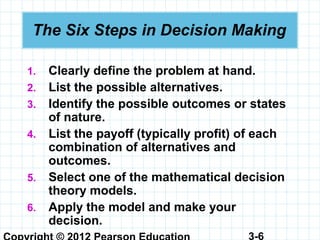
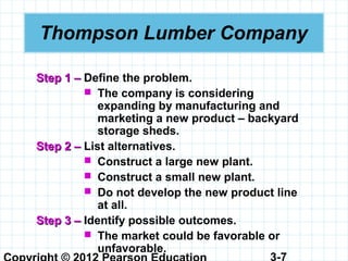
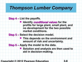
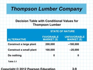
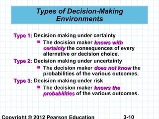
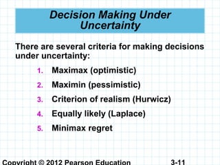
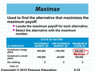
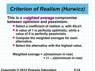
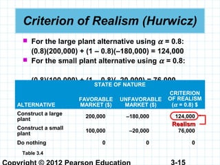
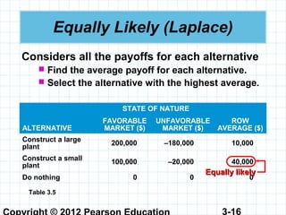
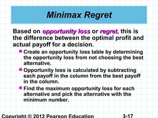
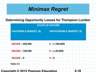
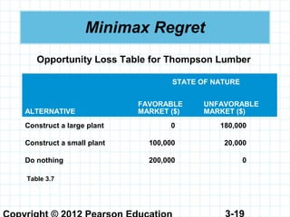
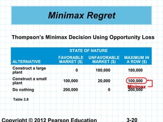
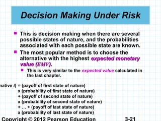
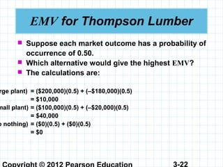
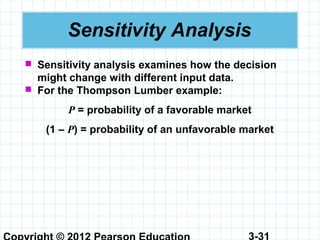
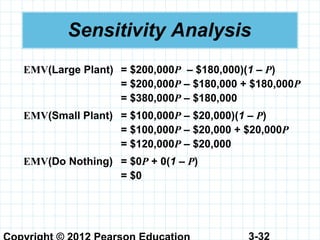
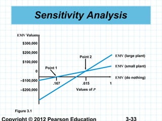
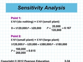
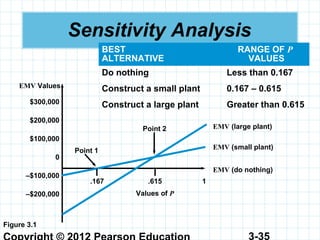
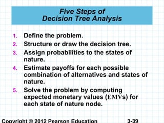
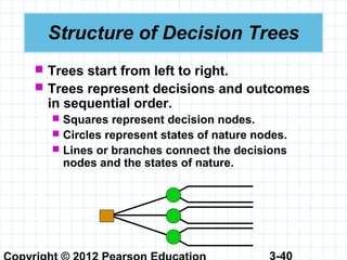
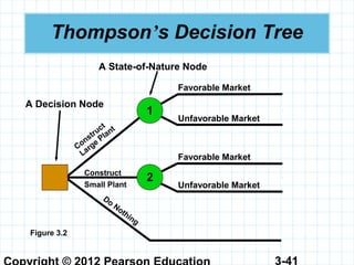
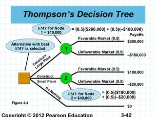
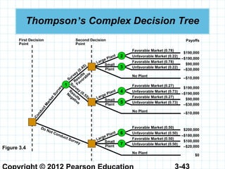
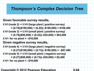
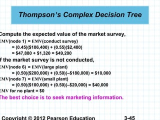
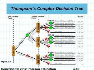
Copyright © 2012 Pearson Education 3-1
Chapter 3
To accompany
Quantitative Analysis for Management, Eleventh Edition, Global Edition
by Render, Stair, and Hanna
Power Point slides created by Brian Peterson
Decision Analysis
3-2
Learning Objectives
1. List the steps of the decision-making
process.
2. Describe the types of decision-making
environments.
3. Make decisions under uncertainty.
4. Use probability values to make decisions
under risk.
After completing this chapter, students will be able to:After completing this chapter, students will be able to:
3-3
Learning Objectives
5. Develop accurate and useful decision
trees.
6. Revise probabilities using Bayesian
analysis.
7. Use computers to solve basic decision-
making problems.
8. Understand the importance and use of
utility theory in decision making.
After completing this chapter, students will be able to:After completing this chapter, students will be able to:
3-4
Chapter Outline
3.1 Introduction
3.2 The Six Steps in Decision Making
3.3 Types of Decision-Making
Environments
3.4 Decision Making under Uncertainty
3.5 Decision Making under Risk
3.6 Decision Trees
3.7 How Probability Values Are
Estimated by Bayesian Analysis
3.8 Utility Theory
3-5
Introduction
 What is involved in making a good
decision?
 Decision theory is an analytic and
systematic approach to the study of
decision making.
 A good decision is one that is based
on logic, considers all available data
and possible alternatives, and the
quantitative approach described here.
3-6
The Six Steps in Decision Making
1. Clearly define the problem at hand.
2. List the possible alternatives.
3. Identify the possible outcomes or states
of nature.
4. List the payoff (typically profit) of each
combination of alternatives and
outcomes.
5. Select one of the mathematical decision
theory models.
6. Apply the model and make your
decision.
3-7
Thompson Lumber Company
Step 1 –Step 1 – Define the problem.
 The company is considering
expanding by manufacturing and
marketing a new product – backyard
storage sheds.
Step 2 –Step 2 – List alternatives.
 Construct a large new plant.
 Construct a small new plant.
 Do not develop the new product line
at all.
Step 3 –Step 3 – Identify possible outcomes.
 The market could be favorable or
unfavorable.
3-8
Thompson Lumber Company
Step 4 –Step 4 – List the payoffs.
 Identify conditional valuesconditional values for the
profits for large plant, small plant, and
no development for the two possible
market conditions.
Step 5 –Step 5 – Select the decision model.
 This depends on the environment and
amount of risk and uncertainty.
Step 6 –Step 6 – Apply the model to the data.
 Solution and analysis are then used to
aid in decision-making.
3-9
Thompson Lumber Company
STATE OF NATURE
ALTERNATIVE
FAVORABLE
MARKET ($)
UNFAVORABLE
MARKET ($)
Construct a large plant 200,000 –180,000
Construct a small plant 100,000 –20,000
Do nothing 0 0
Table 3.1
Decision Table with Conditional Values for
Thompson Lumber
3-10
Types of Decision-Making
Environments
Type 1:Type 1: Decision making under certainty
 The decision maker knows withknows with
certaintycertainty the consequences of every
alternative or decision choice.
Type 2:Type 2: Decision making under uncertainty
 The decision maker does not knowdoes not know the
probabilities of the various outcomes.
Type 3:Type 3: Decision making under risk
 The decision maker knows theknows the
probabilitiesprobabilities of the various outcomes.
3-11
Decision Making Under
Uncertainty
1. Maximax (optimistic)
2. Maximin (pessimistic)
3. Criterion of realism (Hurwicz)
4. Equally likely (Laplace)
5. Minimax regret
There are several criteria for making decisions
under uncertainty:
3-12
Maximax
Used to find the alternative that maximizes the
maximum payoff.
 Locate the maximum payoff for each alternative.
 Select the alternative with the maximum
number.
STATE OF NATURE
ALTERNATIVE
FAVORABLE
MARKET ($)
UNFAVORABLE
MARKET ($)
MAXIMUM IN
A ROW ($)
Construct a large
plant
200,000 –180,000 200,000
Construct a small
plant
100,000 –20,000 100,000
Do nothing 0 0 0
Table 3.2
MaximaxMaximax
3-13
Maximin
Used to find the alternative that maximizes
the minimum payoff.
 Locate the minimum payoff for each alternative.
 Select the alternative with the maximum
number.
STATE OF NATURE
ALTERNATIVE
FAVORABLE
MARKET ($)
UNFAVORABLE
MARKET ($)
MINIMUM IN
A ROW ($)
Construct a large
plant
200,000 –180,000 –180,000
Construct a small
plant
100,000 –20,000 –20,000
Do nothing 0 0 0
Table 3.3 MaximinMaximin
3-14
Criterion of Realism (Hurwicz)
This is a weightedeighted averageaverage compromise
between optimism and pessimism.
 Select a coefficient of realism α, with 0≤α≤1.
 A value of 1 is perfectly optimistic, while a
value of 0 is perfectly pessimistic.
 Compute the weighted averages for each
alternative.
 Select the alternative with the highest value.
Weighted average = α(maximum in row)
+ (1 – α)(minimum in row)
3-15
Criterion of Realism (Hurwicz)
 For the large plant alternative using α = 0.8:
(0.8)(200,000) + (1 – 0.8)(–180,000) = 124,000
 For the small plant alternative using α = 0.8:
(0.8)(100,000) + (1 – 0.8)(–20,000) = 76,000
STATE OF NATURE
ALTERNATIVE
FAVORABLE
MARKET ($)
UNFAVORABLE
MARKET ($)
CRITERION
OF REALISM
(α = 0.8) $
Construct a large
plant
200,000 –180,000 124,000
Construct a small
plant
100,000 –20,000 76,000
Do nothing 0 0 0
Table 3.4
RealismRealism
3-16
Equally Likely (Laplace)
Considers all the payoffs for each alternative
 Find the average payoff for each alternative.
 Select the alternative with the highest average.
STATE OF NATURE
ALTERNATIVE
FAVORABLE
MARKET ($)
UNFAVORABLE
MARKET ($)
ROW
AVERAGE ($)
Construct a large
plant
200,000 –180,000 10,000
Construct a small
plant
100,000 –20,000 40,000
Do nothing 0 0 0
Table 3.5
Equally likelyEqually likely
3-17
Minimax Regret
Based on opportunity lossopportunity loss or regretregret, this is
the difference between the optimal profit and
actual payoff for a decision.
 Create an opportunity loss table by determining
the opportunity loss from not choosing the best
alternative.
 Opportunity loss is calculated by subtracting
each payoff in the column from the best payoff
in the column.
 Find the maximum opportunity loss for each
alternative and pick the alternative with the
minimum number.
3-18
Minimax Regret
STATE OF NATURE
FAVORABLE MARKET ($) UNFAVORABLE MARKET ($)
200,000 – 200,000 0 – (–180,000)
200,000 – 100,000 0 – (–20,000)
200,000 – 0 0 – 0
Table 3.6
Determining Opportunity Losses for Thompson Lumber
3-19
Minimax Regret
Table 3.7
STATE OF NATURE
ALTERNATIVE
FAVORABLE
MARKET ($)
UNFAVORABLE
MARKET ($)
Construct a large plant 0 180,000
Construct a small plant 100,000 20,000
Do nothing 200,000 0
Opportunity Loss Table for Thompson Lumber
3-20
Minimax Regret
Table 3.8
STATE OF NATURE
ALTERNATIVE
FAVORABLE
MARKET ($)
UNFAVORABLE
MARKET ($)
MAXIMUM IN
A ROW ($)
Construct a large
plant
0 180,000 180,000
Construct a small
plant
100,000 20,000 100,000
Do nothing 200,000 0 200,000
MinimaxMinimax
Thompson’s Minimax Decision Using Opportunity Loss
3-21
Decision Making Under Risk
 This is decision making when there are several
possible states of nature, and the probabilities
associated with each possible state are known.
 The most popular method is to choose the
alternative with the highest expected monetaryexpected monetary
value (value (EMVEMV).).
 This is very similar to the expected value calculated in
the last chapter.
native i) = (payoff of first state of nature)
x (probability of first state of nature)
+ (payoff of second state of nature)
x (probability of second state of nature)
+ … + (payoff of last state of nature)
x (probability of last state of nature)
3-22
EMV for Thompson Lumber
 Suppose each market outcome has a probability of
occurrence of 0.50.
 Which alternative would give the highest EMV?
 The calculations are:
rge plant) = ($200,000)(0.5) + (–$180,000)(0.5)
= $10,000
mall plant) = ($100,000)(0.5) + (–$20,000)(0.5)
= $40,000
o nothing) = ($0)(0.5) + ($0)(0.5)
= $0
3-23
EMV for Thompson Lumber
STATE OF NATURE
ALTERNATIVE
FAVORABLE
MARKET ($)
UNFAVORABLE
MARKET ($) EMV ($)
Construct a large
plant
200,000 –180,000 10,000
Construct a small
plant
100,000 –20,000 40,000
Do nothing 0 0 0
Probabilities 0.50 0.50
Table 3.9 LargestLargest EMVEMV
3-24
Expected Value of Perfect
Information (EVPI)
 EVPI places an upper bound on what you should
pay for additional information.
EVPI = EVwPI – Maximum EMV
 EVwPI is the long run average return if we have
perfect information before a decision is made.
EVwPI = (best payoff for first state of nature)
x (probability of first state of nature)
+ (best payoff for second state of nature)
x (probability of second state of nature)
+ … + (best payoff for last state of nature)
x (probability of last state of nature)
3-25
Expected Value of Perfect
Information (EVPI)
 Suppose Scientific Marketing, Inc. offers
analysis that will provide certainty about
market conditions (favorable).
 Additional information will cost $65,000.
 Should Thompson Lumber purchase the
information?
3-26
Expected Value of Perfect
Information (EVPI)
STATE OF NATURE
ALTERNATIVE
FAVORABLE
MARKET ($)
UNFAVORABLE
MARKET ($) EMV ($)
Construct a large
plant
200,000 -180,000 10,000
Construct a small
plant
100,000 -20,000 40,000
Do nothing 0 0 0
With perfect
information
200,000 0 100,000
Probabilities 0.5 0.5
Table 3.10
EVwPIEVwPI
Decision Table with Perfect Information
3-27
Expected Value of Perfect
Information (EVPI)
The maximum EMV without additional information is
$40,000.
EVPI = EVwPI – Maximum EMV
= $100,000 - $40,000
= $60,000
So the maximum Thompson
should pay for the additional
information is $60,000.
3-28
Expected Value of Perfect
Information (EVPI)
The maximum EMV without additional information is
$40,000.
EVPI = EVwPI – Maximum EMV
= $100,000 - $40,000
= $60,000
So the maximum Thompson
should pay for the additional
information is $60,000.
Therefore, Thompson should not
pay $65,000 for this information.
3-29
Expected Opportunity Loss
 Expected opportunity lossExpected opportunity loss (EOL) is the
cost of not picking the best solution.
 First construct an opportunity loss table.
 For each alternative, multiply the
opportunity loss by the probability of that
loss for each possible outcome and add
these together.
 Minimum EOL will always result in the
same decision as maximum EMV.
 Minimum EOL will always equal EVPI.
3-30
Expected Opportunity Loss
arge plant) = (0.50)($0) + (0.50)($180,000)
= $90,000
mall plant) = (0.50)($100,000) + (0.50)($20,000)
= $60,000
o nothing) = (0.50)($200,000) + (0.50)($0)
= $100,000
Table 3.11
STATE OF NATURE
ALTERNATIVE
FAVORABLE
MARKET ($)
UNFAVORABLE
MARKET ($) EOL
Construct a large plant 0 180,000 90,000
Construct a small
plant
100,000 20,000 60,000
Do nothing 200,000 0 100,000
Probabilities 0.50 0.50
MinimumMinimum EOLEOL
3-31
Sensitivity Analysis
 Sensitivity analysis examines how the decision
might change with different input data.
 For the Thompson Lumber example:
P = probability of a favorable market
(1 – P) = probability of an unfavorable market
3-32
Sensitivity Analysis
EMV(Large Plant) = $200,000P – $180,000)(1 – P)
= $200,000P – $180,000 + $180,000P
= $380,000P – $180,000
EMV(Small Plant) = $100,000P – $20,000)(1 – P)
= $100,000P – $20,000 + $20,000P
= $120,000P – $20,000
EMV(Do Nothing) = $0P + 0(1 – P)
= $0
3-33
Sensitivity Analysis
$300,000
$200,000
$100,000
0
–$100,000
–$200,000
EMV Values
EMV (large plant)
EMV (small plant)
EMV (do nothing)
Point 1
Point 2
.167 .615 1
Values of P
Figure 3.1
3-34
Sensitivity Analysis
Point 1:Point 1:
EMV(do nothing) = EMV(small plant)
000200001200 ,$,$ −= P 1670
000120
00020
.
,
,
==P
00018000038000020000120 ,$,$,$,$ −=− PP
6150
000260
000160
.
,
,
==P
Point 2:Point 2:
EMV(small plant) = EMV(large plant)
3-35
Sensitivity Analysis
$300,000
$200,000
$100,000
0
–$100,000
–$200,000
EMV Values
EMV (large plant)
EMV (small plant)
EMV (do nothing)
Point 1
Point 2
.167 .615 1
Values of P
BEST
ALTERNATIVE
RANGE OF P
VALUES
Do nothing Less than 0.167
Construct a small plant 0.167 – 0.615
Construct a large plant Greater than 0.615
Figure 3.1
3-36
Using Excel
Program 3.1A
Input Data for the Thompson Lumber Problem
Using Excel QM
3-37
Using Excel
Program 3.1B
Output Results for the Thompson Lumber Problem
Using Excel QM
3-38
Decision Trees
 Any problem that can be presented in a
decision table can also be graphically
represented in a decision tree.decision tree.
 Decision trees are most beneficial when a
sequence of decisions must be made.
 All decision trees contain decision pointsdecision points
or nodes,nodes, from which one of several alternatives
may be chosen.
 All decision trees contain state-of-naturestate-of-nature
pointspoints or nodes,nodes, out of which one state of
nature will occur.
3-39
Five Steps of
Decision Tree Analysis
1. Define the problem.
2. Structure or draw the decision tree.
3. Assign probabilities to the states of
nature.
4. Estimate payoffs for each possible
combination of alternatives and states of
nature.
5. Solve the problem by computing
expected monetary values (EMVs) for
each state of nature node.
3-40
Structure of Decision Trees
 Trees start from left to right.
 Trees represent decisions and outcomes
in sequential order.
 Squares represent decision nodes.
 Circles represent states of nature nodes.
 Lines or branches connect the decisions
nodes and the states of nature.
3-41
Thompson’s Decision Tree
Favorable Market
Unfavorable Market
Favorable Market
Unfavorable Market
Do
Nothing
Construct
Large
Plant
1
Construct
Small Plant
2
Figure 3.2
A Decision Node
A State-of-Nature Node
3-42
Thompson’s Decision Tree
Favorable Market
Unfavorable Market
Favorable Market
Unfavorable Market
Do
Nothing
Construct
Large
Plant
1
Construct
Small Plant
2
Alternative with best
EMV is selected
Figure 3.3
EMV for Node
1 = $10,000
= (0.5)($200,000) + (0.5)(–$180,000)
EMV for Node
2 = $40,000
= (0.5)($100,000)
+ (0.5)(–$20,000)
Payoffs
$200,000
–$180,000
$100,000
–$20,000
$0
(0.5)
(0.5)
(0.5)
(0.5)
3-43
Thompson’s Complex Decision Tree
First Decision
Point
Second Decision
Point
Favorable Market (0.78)
Unfavorable Market (0.22)
Favorable Market (0.78)
Unfavorable Market (0.22)
Favorable Market (0.27)
Unfavorable Market (0.73)
Favorable Market (0.27)
Unfavorable Market (0.73)
Favorable Market (0.50)
Unfavorable Market (0.50)
Favorable Market (0.50)
Unfavorable Market (0.50)
Large Plant
Small
Plant
No Plant
6
7
ConductM
arketSurvey
Do Not Conduct Survey
Large Plant
Small
Plant
No Plant
2
3
Large Plant
Small
Plant
No Plant
4
5
1
Results
Favorable
Results
Negative
Survey
(0.45)
Survey
(0.55)
Payoffs
–$190,000
$190,000
$90,000
–$30,000
–$10,000
–$180,000
$200,000
$100,000
–$20,000
$0
–$190,000
$190,000
$90,000
–$30,000
–$10,000
Figure 3.4
3-44
Thompson’s Complex Decision Tree
Given favorable survey results,
EMV(node 2) = EMV(large plant | positive survey)
= (0.78)($190,000) + (0.22)(–$190,000) = $106,400
EMV(node 3) = EMV(small plant | positive survey)
= (0.78)($90,000) + (0.22)(–$30,000) = $63,600
EMV for no plant = –$10,000
Given negative survey results,
EMV(node 4) = EMV(large plant | negative survey)
= (0.27)($190,000) + (0.73)(–$190,000) = –$87,400
EMV(node 5) = EMV(small plant | negative survey)
= (0.27)($90,000) + (0.73)(–$30,000) = $2,400
EMV for no plant = –$10,000
3-45
Thompson’s Complex Decision Tree
Compute the expected value of the market survey,
EMV(node 1) = EMV(conduct survey)
= (0.45)($106,400) + (0.55)($2,400)
= $47,880 + $1,320 = $49,200
f the market survey is not conducted,
EMV(node 6) = EMV(large plant)
= (0.50)($200,000) + (0.50)(–$180,000) = $10,000
EMV(node 7) = EMV(small plant)
= (0.50)($100,000) + (0.50)(–$20,000) = $40,000
EMV for no plant = $0
The best choice is to seek marketing information.
3-46
Thompson’s Complex Decision Tree
Figure 3.5
First Decision
Point
Second Decision
Point
Favorable Market (0.78)
Unfavorable Market (0.22)
Favorable Market (0.78)
Unfavorable Market (0.22)
Favorable Market (0.27)
Unfavorable Market (0.73)
Favorable Market (0.27)
Unfavorable Market (0.73)
Favorable Market (0.50)
Unfavorable Market (0.50)
Favorable Market (0.50)
Unfavorable Market (0.50)
Large Plant
Small
Plant
No Plant
ConductM
arketSurvey
Do Not Conduct Survey
Large Plant
Small
Plant
No Plant
Large Plant
Small
Plant
No Plant
Results
Favorable
Results
Negative
Survey
(0.45)
Survey
(0.55)
Payoffs
–$190,000
$190,000
$90,000
–$30,000
–$10,000
–$180,000
$200,000
$100,000
–$20,000
$0
–$190,000
$190,000
$90,000
–$30,000
–$10,000
$40,000$2,400$106,400
$49,200
$106,400
$63,600
–$87,400
$2,400
$10,000
$40,000
3-47
Expected Value of Sample Information
 Suppose Thompson wants to know the
actual value of doing the survey.
EVSI = –
Expected value
withwith sample
information, assuming
no cost to gather it
Expected value
of best decision
withoutwithout sample
information
= (EV with sample information + cost)
– (EV without sample information)
EVSI = ($49,200 + $10,000) – $40,000 = $19,200
3-48
Sensitivity Analysis
 How sensitive are the decisions to
changes in the probabilities?
 How sensitive is our decision to the
probability of a favorable survey result?
 That is, if the probability of a favorable
result (p = .45) where to change, would we
make the same decision?
 How much could it change before we would
make a different decision?
3-49
Sensitivity Analysis
p = probability of a favorable survey
result
(1 – p) = probability of a negative survey
result
EMV(node 1) = ($106,400)p +($2,400)(1 – p)
= $104,000p + $2,400
We are indifferent when the EMV of node 1 is the
same as the EMV of not conducting the survey,
$40,000
$104,000p + $2,400= $40,000
$104,000p = $37,600
p = $37,600/$104,000 = 0.36
If p<0.36, do not conduct the survey. If
p>0.36, conduct the survey.
3-50
Bayesian Analysis
 There are many ways of getting
probability data. It can be based on:
 Management’s experience and intuition.
 Historical data.
 Computed from other data using Bayes’
theorem.
 Bayes’ theorem incorporates initial
estimates and information about the
accuracy of the sources.
 It also allows the revision of initial
estimates based on new information.
3-51
Calculating Revised Probabilities
 In the Thompson Lumber case we used these four
conditional probabilities:
P (favorable market(FM) | survey results positive) = 0.78
P (unfavorable market(UM) | survey results positive) = 0.22
P (favorable market(FM) | survey results negative) = 0.27
P (unfavorable market(UM) | survey results negative) = 0.73
 But how were these calculated?
 The prior probabilities of these markets are:
P (FM) = 0.50
P (UM) = 0.50
3-52
Calculating Revised Probabilities
 Through discussions with experts Thompson has
learned the information in the table below.
 He can use this information and Bayes’ theorem
to calculate posterior probabilities.
STATE OF NATURE
RESULT OF
SURVEY
FAVORABLE MARKET
(FM)
UNFAVORABLE MARKET
(UM)
Positive (predicts
favorable market
for product)
P (survey positive | FM)
= 0.70
P (survey positive | UM)
= 0.20
Negative (predicts
unfavorable
market for
product)
P (survey negative | FM)
= 0.30
P (survey negative | UM)
= 0.80
Table 3.12
3-53
Calculating Revised Probabilities
 Recall Bayes’ theorem:
)()|()()|(
)()|(
)|(
APABPAPABP
APABP
BAP
′×′+×
×
=
where
eventstwoany=BA,
AA ofcomplement=′
For this example, A will represent a favorable
market and B will represent a positive survey.
3-54
Calculating Revised Probabilities
 P (FM | survey positive)
P(UM)|UM)P(P(FM)|FM)P(
FMPFMP
×+×
×
=
positivesurveypositivesurvey
positivesurvey )()|(
780
450
350
500200500700
500700
.
.
.
).)(.().)(.(
).)(.(
==
+
=
P(FM)|FM)P(P(UM)|UM)P(
UMPUMP
×+×
×
=
positivesurveypositivesurvey
positivesurvey )()|(
220
450
100
500700500200
500200
.
.
.
).)(.().)(.(
).)(.(
==
+
=
 P (UM | survey positive)
3-55
Calculating Revised Probabilities
POSTERIOR PROBABILITY
STATE OF
NATURE
CONDITIONAL
PROBABILITY
P(SURVEY
POSITIVE | STATE
OF NATURE)
PRIOR
PROBABILITY
JOINT
PROBABILITY
P(STATE OF
NATURE |
SURVEY
POSITIVE)
FM 0.70 X 0.50 = 0.35 0.35/0.45 = 0.78
UM 0.20 X 0.50 = 0.10 0.10/0.45 = 0.22
P(survey results positive) = 0.45 1.00
Table 3.13
Probability Revisions Given a Positive Survey
3-56
Calculating Revised Probabilities
 P (FM | survey negative)
P(UM)|UM)P(P(FM)|FM)P(
FMPFMP
×+×
×
=
negativesurveynegativesurvey
negativesurvey )()|(
270
550
150
500800500300
500300
.
.
.
).)(.().)(.(
).)(.(
==
+
=
P(FM)|FM)P(P(UM)|UM)P(
UMPUMP
×+×
×
=
negativesurveynegativesurvey
negativesurvey )()|(
730
550
400
500300500800
500800
.
.
.
).)(.().)(.(
).)(.(
==
+
=
 P (UM | survey negative)
3-57
Calculating Revised Probabilities
POSTERIOR PROBABILITY
STATE OF
NATURE
CONDITIONAL
PROBABILITY
P(SURVEY
NEGATIVE | STATE
OF NATURE)
PRIOR
PROBABILITY
JOINT
PROBABILITY
P(STATE OF
NATURE |
SURVEY
NEGATIVE)
FM 0.30 X 0.50 = 0.15 0.15/0.55 = 0.27
UM 0.80 X 0.50 = 0.40 0.40/0.55 = 0.73
P(survey results positive) = 0.55 1.00
Table 3.14
Probability Revisions Given a Negative Survey
3-58
Using Excel
Program 3.2A
Formulas Used for Bayes’ Calculations in Excel
3-59
Using Excel
Program 3.2B
Results of Bayes’ Calculations in Excel
3-60
Potential Problems Using
Survey Results
 We can not always get the necessary
data for analysis.
 Survey results may be based on cases
where an action was taken.
 Conditional probability information
may not be as accurate as we would
like.
3-61
Utility Theory
 Monetary value is not always a true
indicator of the overall value of the
result of a decision.
 The overall value of a decision is called
utility.utility.
 Economists assume that rational
people make decisions to maximize
their utility.
3-62
Heads
(0.5)
Tails
(0.5)
$5,000,000
$0
Utility Theory
Accept
Offer
Reject
Offer
$2,000,000
EMV = $2,500,000Figure 3.6
Your Decision Tree for the Lottery Ticket
3-63
Utility Theory
 Utility assessmentUtility assessment assigns the worst outcome a
utility of 0, and the best outcome, a utility of 1.
 A standard gamblestandard gamble is used to determine utility
values.
 When you are indifferent, your utility values are
equal.
Expected utility of alternative 2 =
Expected utility of alternative 1
Utility of other outcome = (p)
(utility of best outcome, which is 1)
+ (1 – p)(utility of the worst
outcome, which is 0)
Utility of other outcome = (p)
(1) + (1 – p)(0) = p
3-64
Standard Gamble for Utility
Assessment
Best Outcome
Utility = 1
Worst Outcome
Utility = 0
Other Outcome
Utility = ?
(p)
(1 – p)
Alternative 1
Alternative 2
Figure 3.7
3-65
Investment Example
 Jane Dickson wants to construct a utility curve
revealing her preference for money between $0
and $10,000.
 A utility curve plots the utility value versus the
monetary value.
 An investment in a bank will result in $5,000.
 An investment in real estate will result in $0 or
$10,000.
 Unless there is an 80% chance of getting $10,000
from the real estate deal, Jane would prefer to
have her money in the bank.
 So if p = 0.80, Jane is indifferent between the bank
or the real estate investment.
3-66
Investment Example
Figure 3.8
p = 0.80
(1 – p) = 0.20
Invest in
Real Estate
Invest in Bank
$10,000
U($10,000) = 1.0
$0
U($0.00) = 0.0
$5,000
U($5,000) = p = 0.80
Utility for $5,000 = U($5,000) = pU($10,000) + (1 – p)U($0)
= (0.8)(1) + (0.2)(0) = 0.8
3-67
Investment Example
Utility for $7,000 = 0.90
Utility for $3,000 = 0.50
 We can assess other utility values in the same way.
 For Jane these are:
 Using the three utilities for different dollar amounts,
she can construct a utility curve.
3-68
Utility Curve
U ($7,000) = 0.90
U ($5,000) = 0.80
U ($3,000) = 0.50
U ($0) = 0
Figure 3.9
1.0 –
0.9 –
0.8 –
0.7 –
0.6 –
0.5 –
0.4 –
0.3 –
0.2 –
0.1 –
| | | | | | | | | | |
$0 $1,000 $3,000 $5,000 $7,000 $10,000
Monetary Value
Utility
U ($10,000) = 1.0
3-69
Utility Curve
 Jane’s utility curve is typical of a risk avoider.
 She gets less utility from greater risk.
 She avoids situations where high losses might occur.
 As monetary value increases, her utility curve increases
at a slower rate.
 A risk seeker gets more utility from greater risk
 As monetary value increases, the utility curve increases
at a faster rate.
 Someone with risk indifference will have a linear
utility curve.
3-70
Preferences for Risk
Figure 3.10
Monetary Outcome
Utility
Risk
Avoider
R
isk
Indifference
Risk
Seeker
3-71
Utility as a
Decision-Making Criteria
 Once a utility curve has been developed
it can be used in making decisions.
 This replaces monetary outcomes with
utility values.
 The expected utility is computed instead
of the EMV.
3-72
Utility as a
Decision-Making Criteria
 Mark Simkin loves to gamble.
 He plays a game tossing thumbtacks in
the air.
 If the thumbtack lands point up, Mark wins
$10,000.
 If the thumbtack lands point down, Mark
loses $10,000.
 Mark believes that there is a 45% chance
the thumbtack will land point up.
 Should Mark play the game (alternative 1)?
3-73
Utility as a
Decision-Making Criteria
Figure 3.11
Tack Lands
Point Up (0.45)
Alternative 1
Mark Plays the Game
Alternative 2
$10,000
–$10,000
$0
Tack Lands
Point Down (0.55)
Mark Does Not Play the Game
Decision Facing Mark Simkin
3-74
Utility as a
Decision-Making Criteria
 Step 1– Define Mark’s utilities.
U (–$10,000) = 0.05
U ($0) = 0.15
U ($10,000) = 0.30
 Step 2 – Replace monetary values with
utility values.
E(alternative 1: play the game) = (0.45)(0.30) + (0.55)(0.05)
= 0.135 + 0.027 = 0.162
E(alternative 2: don’t play the game) = 0.15
3-75
Utility Curve for Mark Simkin
Figure 3.12
1.00 –
0.75 –
0.50 –
0.30 –
0.25 –
0.15 –
0.05 –
0 –| | | | |
–$20,000 –$10,000 $0 $10,000 $20,000
Monetary Outcome
Utility
3-76
Utility as a
Decision-Making Criteria
Figure 3.13
Tack Lands
Point Up (0.45)
Alternative 1
Mark Plays the Game
Alternative 2
0.30
0.05
0.15
Tack Lands
Point Down (0.55)
Don’t Play
UtilityE = 0.162
Using Expected Utilities in Decision Making
3-77
Copyright
All rights reserved. No part of this publication may be
reproduced, stored in a retrieval system, or transmitted, in
any form or by any means, electronic, mechanical,
photocopying, recording, or otherwise, without the prior
written permission of the publisher. Printed in the United
States of America.

Rsh qam11 ch03 ge

  • 1.
    Copyright © 2012Pearson Education 3-1 Chapter 3 To accompany Quantitative Analysis for Management, Eleventh Edition, Global Edition by Render, Stair, and Hanna Power Point slides created by Brian Peterson Decision Analysis
  • 2.
    3-2 Learning Objectives 1. Listthe steps of the decision-making process. 2. Describe the types of decision-making environments. 3. Make decisions under uncertainty. 4. Use probability values to make decisions under risk. After completing this chapter, students will be able to:After completing this chapter, students will be able to:
  • 3.
    3-3 Learning Objectives 5. Developaccurate and useful decision trees. 6. Revise probabilities using Bayesian analysis. 7. Use computers to solve basic decision- making problems. 8. Understand the importance and use of utility theory in decision making. After completing this chapter, students will be able to:After completing this chapter, students will be able to:
  • 4.
    3-4 Chapter Outline 3.1 Introduction 3.2The Six Steps in Decision Making 3.3 Types of Decision-Making Environments 3.4 Decision Making under Uncertainty 3.5 Decision Making under Risk 3.6 Decision Trees 3.7 How Probability Values Are Estimated by Bayesian Analysis 3.8 Utility Theory
  • 5.
    3-5 Introduction  What isinvolved in making a good decision?  Decision theory is an analytic and systematic approach to the study of decision making.  A good decision is one that is based on logic, considers all available data and possible alternatives, and the quantitative approach described here.
  • 6.
    3-6 The Six Stepsin Decision Making 1. Clearly define the problem at hand. 2. List the possible alternatives. 3. Identify the possible outcomes or states of nature. 4. List the payoff (typically profit) of each combination of alternatives and outcomes. 5. Select one of the mathematical decision theory models. 6. Apply the model and make your decision.
  • 7.
    3-7 Thompson Lumber Company Step1 –Step 1 – Define the problem.  The company is considering expanding by manufacturing and marketing a new product – backyard storage sheds. Step 2 –Step 2 – List alternatives.  Construct a large new plant.  Construct a small new plant.  Do not develop the new product line at all. Step 3 –Step 3 – Identify possible outcomes.  The market could be favorable or unfavorable.
  • 8.
    3-8 Thompson Lumber Company Step4 –Step 4 – List the payoffs.  Identify conditional valuesconditional values for the profits for large plant, small plant, and no development for the two possible market conditions. Step 5 –Step 5 – Select the decision model.  This depends on the environment and amount of risk and uncertainty. Step 6 –Step 6 – Apply the model to the data.  Solution and analysis are then used to aid in decision-making.
  • 9.
    3-9 Thompson Lumber Company STATEOF NATURE ALTERNATIVE FAVORABLE MARKET ($) UNFAVORABLE MARKET ($) Construct a large plant 200,000 –180,000 Construct a small plant 100,000 –20,000 Do nothing 0 0 Table 3.1 Decision Table with Conditional Values for Thompson Lumber
  • 10.
    3-10 Types of Decision-Making Environments Type1:Type 1: Decision making under certainty  The decision maker knows withknows with certaintycertainty the consequences of every alternative or decision choice. Type 2:Type 2: Decision making under uncertainty  The decision maker does not knowdoes not know the probabilities of the various outcomes. Type 3:Type 3: Decision making under risk  The decision maker knows theknows the probabilitiesprobabilities of the various outcomes.
  • 11.
    3-11 Decision Making Under Uncertainty 1.Maximax (optimistic) 2. Maximin (pessimistic) 3. Criterion of realism (Hurwicz) 4. Equally likely (Laplace) 5. Minimax regret There are several criteria for making decisions under uncertainty:
  • 12.
    3-12 Maximax Used to findthe alternative that maximizes the maximum payoff.  Locate the maximum payoff for each alternative.  Select the alternative with the maximum number. STATE OF NATURE ALTERNATIVE FAVORABLE MARKET ($) UNFAVORABLE MARKET ($) MAXIMUM IN A ROW ($) Construct a large plant 200,000 –180,000 200,000 Construct a small plant 100,000 –20,000 100,000 Do nothing 0 0 0 Table 3.2 MaximaxMaximax
  • 13.
    3-13 Maximin Used to findthe alternative that maximizes the minimum payoff.  Locate the minimum payoff for each alternative.  Select the alternative with the maximum number. STATE OF NATURE ALTERNATIVE FAVORABLE MARKET ($) UNFAVORABLE MARKET ($) MINIMUM IN A ROW ($) Construct a large plant 200,000 –180,000 –180,000 Construct a small plant 100,000 –20,000 –20,000 Do nothing 0 0 0 Table 3.3 MaximinMaximin
  • 14.
    3-14 Criterion of Realism(Hurwicz) This is a weightedeighted averageaverage compromise between optimism and pessimism.  Select a coefficient of realism α, with 0≤α≤1.  A value of 1 is perfectly optimistic, while a value of 0 is perfectly pessimistic.  Compute the weighted averages for each alternative.  Select the alternative with the highest value. Weighted average = α(maximum in row) + (1 – α)(minimum in row)
  • 15.
    3-15 Criterion of Realism(Hurwicz)  For the large plant alternative using α = 0.8: (0.8)(200,000) + (1 – 0.8)(–180,000) = 124,000  For the small plant alternative using α = 0.8: (0.8)(100,000) + (1 – 0.8)(–20,000) = 76,000 STATE OF NATURE ALTERNATIVE FAVORABLE MARKET ($) UNFAVORABLE MARKET ($) CRITERION OF REALISM (α = 0.8) $ Construct a large plant 200,000 –180,000 124,000 Construct a small plant 100,000 –20,000 76,000 Do nothing 0 0 0 Table 3.4 RealismRealism
  • 16.
    3-16 Equally Likely (Laplace) Considersall the payoffs for each alternative  Find the average payoff for each alternative.  Select the alternative with the highest average. STATE OF NATURE ALTERNATIVE FAVORABLE MARKET ($) UNFAVORABLE MARKET ($) ROW AVERAGE ($) Construct a large plant 200,000 –180,000 10,000 Construct a small plant 100,000 –20,000 40,000 Do nothing 0 0 0 Table 3.5 Equally likelyEqually likely
  • 17.
    3-17 Minimax Regret Based onopportunity lossopportunity loss or regretregret, this is the difference between the optimal profit and actual payoff for a decision.  Create an opportunity loss table by determining the opportunity loss from not choosing the best alternative.  Opportunity loss is calculated by subtracting each payoff in the column from the best payoff in the column.  Find the maximum opportunity loss for each alternative and pick the alternative with the minimum number.
  • 18.
    3-18 Minimax Regret STATE OFNATURE FAVORABLE MARKET ($) UNFAVORABLE MARKET ($) 200,000 – 200,000 0 – (–180,000) 200,000 – 100,000 0 – (–20,000) 200,000 – 0 0 – 0 Table 3.6 Determining Opportunity Losses for Thompson Lumber
  • 19.
    3-19 Minimax Regret Table 3.7 STATEOF NATURE ALTERNATIVE FAVORABLE MARKET ($) UNFAVORABLE MARKET ($) Construct a large plant 0 180,000 Construct a small plant 100,000 20,000 Do nothing 200,000 0 Opportunity Loss Table for Thompson Lumber
  • 20.
    3-20 Minimax Regret Table 3.8 STATEOF NATURE ALTERNATIVE FAVORABLE MARKET ($) UNFAVORABLE MARKET ($) MAXIMUM IN A ROW ($) Construct a large plant 0 180,000 180,000 Construct a small plant 100,000 20,000 100,000 Do nothing 200,000 0 200,000 MinimaxMinimax Thompson’s Minimax Decision Using Opportunity Loss
  • 21.
    3-21 Decision Making UnderRisk  This is decision making when there are several possible states of nature, and the probabilities associated with each possible state are known.  The most popular method is to choose the alternative with the highest expected monetaryexpected monetary value (value (EMVEMV).).  This is very similar to the expected value calculated in the last chapter. native i) = (payoff of first state of nature) x (probability of first state of nature) + (payoff of second state of nature) x (probability of second state of nature) + … + (payoff of last state of nature) x (probability of last state of nature)
  • 22.
    3-22 EMV for ThompsonLumber  Suppose each market outcome has a probability of occurrence of 0.50.  Which alternative would give the highest EMV?  The calculations are: rge plant) = ($200,000)(0.5) + (–$180,000)(0.5) = $10,000 mall plant) = ($100,000)(0.5) + (–$20,000)(0.5) = $40,000 o nothing) = ($0)(0.5) + ($0)(0.5) = $0
  • 23.
    3-23 EMV for ThompsonLumber STATE OF NATURE ALTERNATIVE FAVORABLE MARKET ($) UNFAVORABLE MARKET ($) EMV ($) Construct a large plant 200,000 –180,000 10,000 Construct a small plant 100,000 –20,000 40,000 Do nothing 0 0 0 Probabilities 0.50 0.50 Table 3.9 LargestLargest EMVEMV
  • 24.
    3-24 Expected Value ofPerfect Information (EVPI)  EVPI places an upper bound on what you should pay for additional information. EVPI = EVwPI – Maximum EMV  EVwPI is the long run average return if we have perfect information before a decision is made. EVwPI = (best payoff for first state of nature) x (probability of first state of nature) + (best payoff for second state of nature) x (probability of second state of nature) + … + (best payoff for last state of nature) x (probability of last state of nature)
  • 25.
    3-25 Expected Value ofPerfect Information (EVPI)  Suppose Scientific Marketing, Inc. offers analysis that will provide certainty about market conditions (favorable).  Additional information will cost $65,000.  Should Thompson Lumber purchase the information?
  • 26.
    3-26 Expected Value ofPerfect Information (EVPI) STATE OF NATURE ALTERNATIVE FAVORABLE MARKET ($) UNFAVORABLE MARKET ($) EMV ($) Construct a large plant 200,000 -180,000 10,000 Construct a small plant 100,000 -20,000 40,000 Do nothing 0 0 0 With perfect information 200,000 0 100,000 Probabilities 0.5 0.5 Table 3.10 EVwPIEVwPI Decision Table with Perfect Information
  • 27.
    3-27 Expected Value ofPerfect Information (EVPI) The maximum EMV without additional information is $40,000. EVPI = EVwPI – Maximum EMV = $100,000 - $40,000 = $60,000 So the maximum Thompson should pay for the additional information is $60,000.
  • 28.
    3-28 Expected Value ofPerfect Information (EVPI) The maximum EMV without additional information is $40,000. EVPI = EVwPI – Maximum EMV = $100,000 - $40,000 = $60,000 So the maximum Thompson should pay for the additional information is $60,000. Therefore, Thompson should not pay $65,000 for this information.
  • 29.
    3-29 Expected Opportunity Loss Expected opportunity lossExpected opportunity loss (EOL) is the cost of not picking the best solution.  First construct an opportunity loss table.  For each alternative, multiply the opportunity loss by the probability of that loss for each possible outcome and add these together.  Minimum EOL will always result in the same decision as maximum EMV.  Minimum EOL will always equal EVPI.
  • 30.
    3-30 Expected Opportunity Loss argeplant) = (0.50)($0) + (0.50)($180,000) = $90,000 mall plant) = (0.50)($100,000) + (0.50)($20,000) = $60,000 o nothing) = (0.50)($200,000) + (0.50)($0) = $100,000 Table 3.11 STATE OF NATURE ALTERNATIVE FAVORABLE MARKET ($) UNFAVORABLE MARKET ($) EOL Construct a large plant 0 180,000 90,000 Construct a small plant 100,000 20,000 60,000 Do nothing 200,000 0 100,000 Probabilities 0.50 0.50 MinimumMinimum EOLEOL
  • 31.
    3-31 Sensitivity Analysis  Sensitivityanalysis examines how the decision might change with different input data.  For the Thompson Lumber example: P = probability of a favorable market (1 – P) = probability of an unfavorable market
  • 32.
    3-32 Sensitivity Analysis EMV(Large Plant)= $200,000P – $180,000)(1 – P) = $200,000P – $180,000 + $180,000P = $380,000P – $180,000 EMV(Small Plant) = $100,000P – $20,000)(1 – P) = $100,000P – $20,000 + $20,000P = $120,000P – $20,000 EMV(Do Nothing) = $0P + 0(1 – P) = $0
  • 33.
    3-33 Sensitivity Analysis $300,000 $200,000 $100,000 0 –$100,000 –$200,000 EMV Values EMV(large plant) EMV (small plant) EMV (do nothing) Point 1 Point 2 .167 .615 1 Values of P Figure 3.1
  • 34.
    3-34 Sensitivity Analysis Point 1:Point1: EMV(do nothing) = EMV(small plant) 000200001200 ,$,$ −= P 1670 000120 00020 . , , ==P 00018000038000020000120 ,$,$,$,$ −=− PP 6150 000260 000160 . , , ==P Point 2:Point 2: EMV(small plant) = EMV(large plant)
  • 35.
    3-35 Sensitivity Analysis $300,000 $200,000 $100,000 0 –$100,000 –$200,000 EMV Values EMV(large plant) EMV (small plant) EMV (do nothing) Point 1 Point 2 .167 .615 1 Values of P BEST ALTERNATIVE RANGE OF P VALUES Do nothing Less than 0.167 Construct a small plant 0.167 – 0.615 Construct a large plant Greater than 0.615 Figure 3.1
  • 36.
    3-36 Using Excel Program 3.1A InputData for the Thompson Lumber Problem Using Excel QM
  • 37.
    3-37 Using Excel Program 3.1B OutputResults for the Thompson Lumber Problem Using Excel QM
  • 38.
    3-38 Decision Trees  Anyproblem that can be presented in a decision table can also be graphically represented in a decision tree.decision tree.  Decision trees are most beneficial when a sequence of decisions must be made.  All decision trees contain decision pointsdecision points or nodes,nodes, from which one of several alternatives may be chosen.  All decision trees contain state-of-naturestate-of-nature pointspoints or nodes,nodes, out of which one state of nature will occur.
  • 39.
    3-39 Five Steps of DecisionTree Analysis 1. Define the problem. 2. Structure or draw the decision tree. 3. Assign probabilities to the states of nature. 4. Estimate payoffs for each possible combination of alternatives and states of nature. 5. Solve the problem by computing expected monetary values (EMVs) for each state of nature node.
  • 40.
    3-40 Structure of DecisionTrees  Trees start from left to right.  Trees represent decisions and outcomes in sequential order.  Squares represent decision nodes.  Circles represent states of nature nodes.  Lines or branches connect the decisions nodes and the states of nature.
  • 41.
    3-41 Thompson’s Decision Tree FavorableMarket Unfavorable Market Favorable Market Unfavorable Market Do Nothing Construct Large Plant 1 Construct Small Plant 2 Figure 3.2 A Decision Node A State-of-Nature Node
  • 42.
    3-42 Thompson’s Decision Tree FavorableMarket Unfavorable Market Favorable Market Unfavorable Market Do Nothing Construct Large Plant 1 Construct Small Plant 2 Alternative with best EMV is selected Figure 3.3 EMV for Node 1 = $10,000 = (0.5)($200,000) + (0.5)(–$180,000) EMV for Node 2 = $40,000 = (0.5)($100,000) + (0.5)(–$20,000) Payoffs $200,000 –$180,000 $100,000 –$20,000 $0 (0.5) (0.5) (0.5) (0.5)
  • 43.
    3-43 Thompson’s Complex DecisionTree First Decision Point Second Decision Point Favorable Market (0.78) Unfavorable Market (0.22) Favorable Market (0.78) Unfavorable Market (0.22) Favorable Market (0.27) Unfavorable Market (0.73) Favorable Market (0.27) Unfavorable Market (0.73) Favorable Market (0.50) Unfavorable Market (0.50) Favorable Market (0.50) Unfavorable Market (0.50) Large Plant Small Plant No Plant 6 7 ConductM arketSurvey Do Not Conduct Survey Large Plant Small Plant No Plant 2 3 Large Plant Small Plant No Plant 4 5 1 Results Favorable Results Negative Survey (0.45) Survey (0.55) Payoffs –$190,000 $190,000 $90,000 –$30,000 –$10,000 –$180,000 $200,000 $100,000 –$20,000 $0 –$190,000 $190,000 $90,000 –$30,000 –$10,000 Figure 3.4
  • 44.
    3-44 Thompson’s Complex DecisionTree Given favorable survey results, EMV(node 2) = EMV(large plant | positive survey) = (0.78)($190,000) + (0.22)(–$190,000) = $106,400 EMV(node 3) = EMV(small plant | positive survey) = (0.78)($90,000) + (0.22)(–$30,000) = $63,600 EMV for no plant = –$10,000 Given negative survey results, EMV(node 4) = EMV(large plant | negative survey) = (0.27)($190,000) + (0.73)(–$190,000) = –$87,400 EMV(node 5) = EMV(small plant | negative survey) = (0.27)($90,000) + (0.73)(–$30,000) = $2,400 EMV for no plant = –$10,000
  • 45.
    3-45 Thompson’s Complex DecisionTree Compute the expected value of the market survey, EMV(node 1) = EMV(conduct survey) = (0.45)($106,400) + (0.55)($2,400) = $47,880 + $1,320 = $49,200 f the market survey is not conducted, EMV(node 6) = EMV(large plant) = (0.50)($200,000) + (0.50)(–$180,000) = $10,000 EMV(node 7) = EMV(small plant) = (0.50)($100,000) + (0.50)(–$20,000) = $40,000 EMV for no plant = $0 The best choice is to seek marketing information.
  • 46.
    3-46 Thompson’s Complex DecisionTree Figure 3.5 First Decision Point Second Decision Point Favorable Market (0.78) Unfavorable Market (0.22) Favorable Market (0.78) Unfavorable Market (0.22) Favorable Market (0.27) Unfavorable Market (0.73) Favorable Market (0.27) Unfavorable Market (0.73) Favorable Market (0.50) Unfavorable Market (0.50) Favorable Market (0.50) Unfavorable Market (0.50) Large Plant Small Plant No Plant ConductM arketSurvey Do Not Conduct Survey Large Plant Small Plant No Plant Large Plant Small Plant No Plant Results Favorable Results Negative Survey (0.45) Survey (0.55) Payoffs –$190,000 $190,000 $90,000 –$30,000 –$10,000 –$180,000 $200,000 $100,000 –$20,000 $0 –$190,000 $190,000 $90,000 –$30,000 –$10,000 $40,000$2,400$106,400 $49,200 $106,400 $63,600 –$87,400 $2,400 $10,000 $40,000
  • 47.
    3-47 Expected Value ofSample Information  Suppose Thompson wants to know the actual value of doing the survey. EVSI = – Expected value withwith sample information, assuming no cost to gather it Expected value of best decision withoutwithout sample information = (EV with sample information + cost) – (EV without sample information) EVSI = ($49,200 + $10,000) – $40,000 = $19,200
  • 48.
    3-48 Sensitivity Analysis  Howsensitive are the decisions to changes in the probabilities?  How sensitive is our decision to the probability of a favorable survey result?  That is, if the probability of a favorable result (p = .45) where to change, would we make the same decision?  How much could it change before we would make a different decision?
  • 49.
    3-49 Sensitivity Analysis p =probability of a favorable survey result (1 – p) = probability of a negative survey result EMV(node 1) = ($106,400)p +($2,400)(1 – p) = $104,000p + $2,400 We are indifferent when the EMV of node 1 is the same as the EMV of not conducting the survey, $40,000 $104,000p + $2,400= $40,000 $104,000p = $37,600 p = $37,600/$104,000 = 0.36 If p<0.36, do not conduct the survey. If p>0.36, conduct the survey.
  • 50.
    3-50 Bayesian Analysis  Thereare many ways of getting probability data. It can be based on:  Management’s experience and intuition.  Historical data.  Computed from other data using Bayes’ theorem.  Bayes’ theorem incorporates initial estimates and information about the accuracy of the sources.  It also allows the revision of initial estimates based on new information.
  • 51.
    3-51 Calculating Revised Probabilities In the Thompson Lumber case we used these four conditional probabilities: P (favorable market(FM) | survey results positive) = 0.78 P (unfavorable market(UM) | survey results positive) = 0.22 P (favorable market(FM) | survey results negative) = 0.27 P (unfavorable market(UM) | survey results negative) = 0.73  But how were these calculated?  The prior probabilities of these markets are: P (FM) = 0.50 P (UM) = 0.50
  • 52.
    3-52 Calculating Revised Probabilities Through discussions with experts Thompson has learned the information in the table below.  He can use this information and Bayes’ theorem to calculate posterior probabilities. STATE OF NATURE RESULT OF SURVEY FAVORABLE MARKET (FM) UNFAVORABLE MARKET (UM) Positive (predicts favorable market for product) P (survey positive | FM) = 0.70 P (survey positive | UM) = 0.20 Negative (predicts unfavorable market for product) P (survey negative | FM) = 0.30 P (survey negative | UM) = 0.80 Table 3.12
  • 53.
    3-53 Calculating Revised Probabilities Recall Bayes’ theorem: )()|()()|( )()|( )|( APABPAPABP APABP BAP ′×′+× × = where eventstwoany=BA, AA ofcomplement=′ For this example, A will represent a favorable market and B will represent a positive survey.
  • 54.
    3-54 Calculating Revised Probabilities P (FM | survey positive) P(UM)|UM)P(P(FM)|FM)P( FMPFMP ×+× × = positivesurveypositivesurvey positivesurvey )()|( 780 450 350 500200500700 500700 . . . ).)(.().)(.( ).)(.( == + = P(FM)|FM)P(P(UM)|UM)P( UMPUMP ×+× × = positivesurveypositivesurvey positivesurvey )()|( 220 450 100 500700500200 500200 . . . ).)(.().)(.( ).)(.( == + =  P (UM | survey positive)
  • 55.
    3-55 Calculating Revised Probabilities POSTERIORPROBABILITY STATE OF NATURE CONDITIONAL PROBABILITY P(SURVEY POSITIVE | STATE OF NATURE) PRIOR PROBABILITY JOINT PROBABILITY P(STATE OF NATURE | SURVEY POSITIVE) FM 0.70 X 0.50 = 0.35 0.35/0.45 = 0.78 UM 0.20 X 0.50 = 0.10 0.10/0.45 = 0.22 P(survey results positive) = 0.45 1.00 Table 3.13 Probability Revisions Given a Positive Survey
  • 56.
    3-56 Calculating Revised Probabilities P (FM | survey negative) P(UM)|UM)P(P(FM)|FM)P( FMPFMP ×+× × = negativesurveynegativesurvey negativesurvey )()|( 270 550 150 500800500300 500300 . . . ).)(.().)(.( ).)(.( == + = P(FM)|FM)P(P(UM)|UM)P( UMPUMP ×+× × = negativesurveynegativesurvey negativesurvey )()|( 730 550 400 500300500800 500800 . . . ).)(.().)(.( ).)(.( == + =  P (UM | survey negative)
  • 57.
    3-57 Calculating Revised Probabilities POSTERIORPROBABILITY STATE OF NATURE CONDITIONAL PROBABILITY P(SURVEY NEGATIVE | STATE OF NATURE) PRIOR PROBABILITY JOINT PROBABILITY P(STATE OF NATURE | SURVEY NEGATIVE) FM 0.30 X 0.50 = 0.15 0.15/0.55 = 0.27 UM 0.80 X 0.50 = 0.40 0.40/0.55 = 0.73 P(survey results positive) = 0.55 1.00 Table 3.14 Probability Revisions Given a Negative Survey
  • 58.
    3-58 Using Excel Program 3.2A FormulasUsed for Bayes’ Calculations in Excel
  • 59.
    3-59 Using Excel Program 3.2B Resultsof Bayes’ Calculations in Excel
  • 60.
    3-60 Potential Problems Using SurveyResults  We can not always get the necessary data for analysis.  Survey results may be based on cases where an action was taken.  Conditional probability information may not be as accurate as we would like.
  • 61.
    3-61 Utility Theory  Monetaryvalue is not always a true indicator of the overall value of the result of a decision.  The overall value of a decision is called utility.utility.  Economists assume that rational people make decisions to maximize their utility.
  • 62.
  • 63.
    3-63 Utility Theory  UtilityassessmentUtility assessment assigns the worst outcome a utility of 0, and the best outcome, a utility of 1.  A standard gamblestandard gamble is used to determine utility values.  When you are indifferent, your utility values are equal. Expected utility of alternative 2 = Expected utility of alternative 1 Utility of other outcome = (p) (utility of best outcome, which is 1) + (1 – p)(utility of the worst outcome, which is 0) Utility of other outcome = (p) (1) + (1 – p)(0) = p
  • 64.
    3-64 Standard Gamble forUtility Assessment Best Outcome Utility = 1 Worst Outcome Utility = 0 Other Outcome Utility = ? (p) (1 – p) Alternative 1 Alternative 2 Figure 3.7
  • 65.
    3-65 Investment Example  JaneDickson wants to construct a utility curve revealing her preference for money between $0 and $10,000.  A utility curve plots the utility value versus the monetary value.  An investment in a bank will result in $5,000.  An investment in real estate will result in $0 or $10,000.  Unless there is an 80% chance of getting $10,000 from the real estate deal, Jane would prefer to have her money in the bank.  So if p = 0.80, Jane is indifferent between the bank or the real estate investment.
  • 66.
    3-66 Investment Example Figure 3.8 p= 0.80 (1 – p) = 0.20 Invest in Real Estate Invest in Bank $10,000 U($10,000) = 1.0 $0 U($0.00) = 0.0 $5,000 U($5,000) = p = 0.80 Utility for $5,000 = U($5,000) = pU($10,000) + (1 – p)U($0) = (0.8)(1) + (0.2)(0) = 0.8
  • 67.
    3-67 Investment Example Utility for$7,000 = 0.90 Utility for $3,000 = 0.50  We can assess other utility values in the same way.  For Jane these are:  Using the three utilities for different dollar amounts, she can construct a utility curve.
  • 68.
    3-68 Utility Curve U ($7,000)= 0.90 U ($5,000) = 0.80 U ($3,000) = 0.50 U ($0) = 0 Figure 3.9 1.0 – 0.9 – 0.8 – 0.7 – 0.6 – 0.5 – 0.4 – 0.3 – 0.2 – 0.1 – | | | | | | | | | | | $0 $1,000 $3,000 $5,000 $7,000 $10,000 Monetary Value Utility U ($10,000) = 1.0
  • 69.
    3-69 Utility Curve  Jane’sutility curve is typical of a risk avoider.  She gets less utility from greater risk.  She avoids situations where high losses might occur.  As monetary value increases, her utility curve increases at a slower rate.  A risk seeker gets more utility from greater risk  As monetary value increases, the utility curve increases at a faster rate.  Someone with risk indifference will have a linear utility curve.
  • 70.
    3-70 Preferences for Risk Figure3.10 Monetary Outcome Utility Risk Avoider R isk Indifference Risk Seeker
  • 71.
    3-71 Utility as a Decision-MakingCriteria  Once a utility curve has been developed it can be used in making decisions.  This replaces monetary outcomes with utility values.  The expected utility is computed instead of the EMV.
  • 72.
    3-72 Utility as a Decision-MakingCriteria  Mark Simkin loves to gamble.  He plays a game tossing thumbtacks in the air.  If the thumbtack lands point up, Mark wins $10,000.  If the thumbtack lands point down, Mark loses $10,000.  Mark believes that there is a 45% chance the thumbtack will land point up.  Should Mark play the game (alternative 1)?
  • 73.
    3-73 Utility as a Decision-MakingCriteria Figure 3.11 Tack Lands Point Up (0.45) Alternative 1 Mark Plays the Game Alternative 2 $10,000 –$10,000 $0 Tack Lands Point Down (0.55) Mark Does Not Play the Game Decision Facing Mark Simkin
  • 74.
    3-74 Utility as a Decision-MakingCriteria  Step 1– Define Mark’s utilities. U (–$10,000) = 0.05 U ($0) = 0.15 U ($10,000) = 0.30  Step 2 – Replace monetary values with utility values. E(alternative 1: play the game) = (0.45)(0.30) + (0.55)(0.05) = 0.135 + 0.027 = 0.162 E(alternative 2: don’t play the game) = 0.15
  • 75.
    3-75 Utility Curve forMark Simkin Figure 3.12 1.00 – 0.75 – 0.50 – 0.30 – 0.25 – 0.15 – 0.05 – 0 –| | | | | –$20,000 –$10,000 $0 $10,000 $20,000 Monetary Outcome Utility
  • 76.
    3-76 Utility as a Decision-MakingCriteria Figure 3.13 Tack Lands Point Up (0.45) Alternative 1 Mark Plays the Game Alternative 2 0.30 0.05 0.15 Tack Lands Point Down (0.55) Don’t Play UtilityE = 0.162 Using Expected Utilities in Decision Making
  • 77.
    3-77 Copyright All rights reserved.No part of this publication may be reproduced, stored in a retrieval system, or transmitted, in any form or by any means, electronic, mechanical, photocopying, recording, or otherwise, without the prior written permission of the publisher. Printed in the United States of America.