Downloaded 485 times
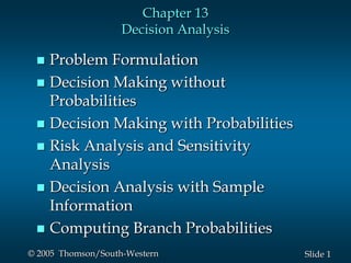


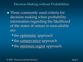
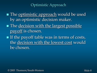
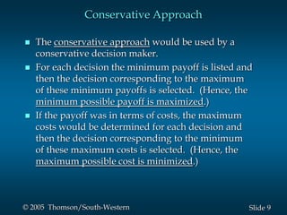
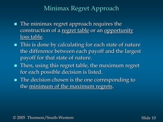
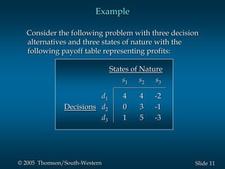
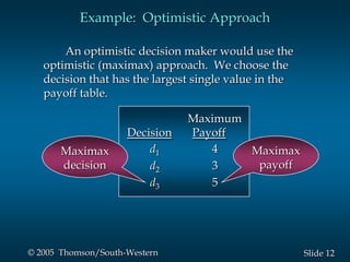
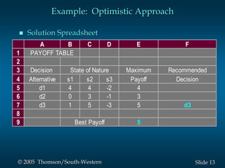
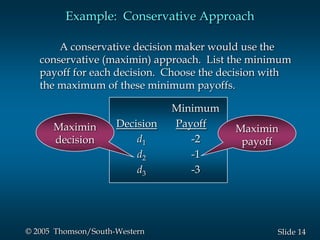
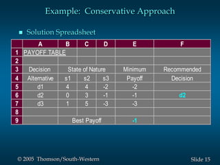
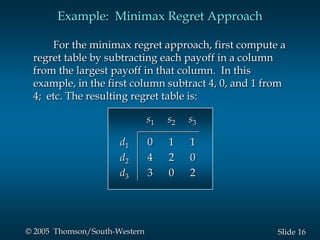
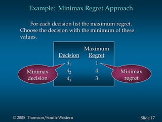
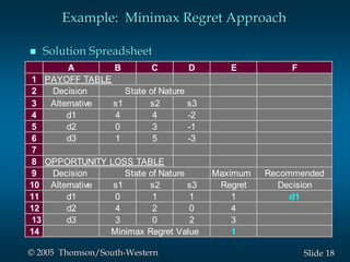

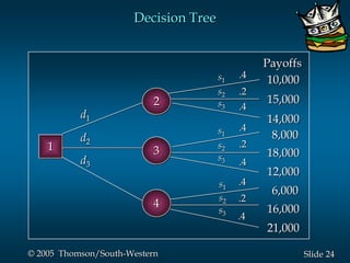
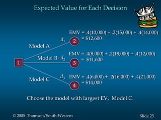
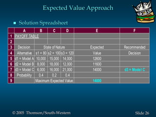

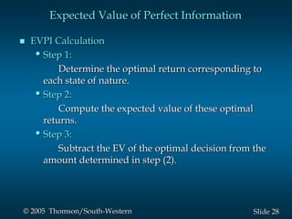
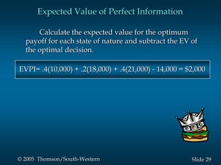
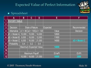
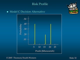

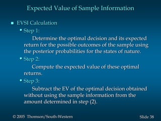
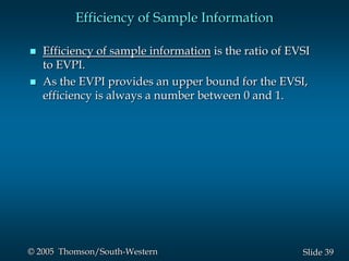
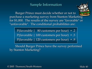
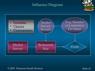
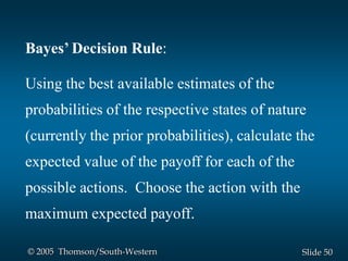
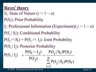


This document provides an overview of key concepts in decision analysis, including problem formulation, decision making without and with probabilities, risk analysis, sensitivity analysis, and computing branch probabilities. It discusses techniques like influence diagrams, payoff tables, decision trees, and the expected value, conservative, optimistic, and minimax regret approaches. It also covers risk profiles, sensitivity analysis, Bayes' theorem, and the expected value of perfect and sample information.