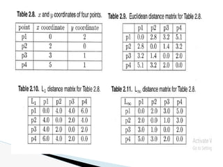
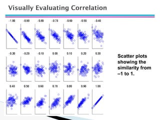
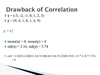
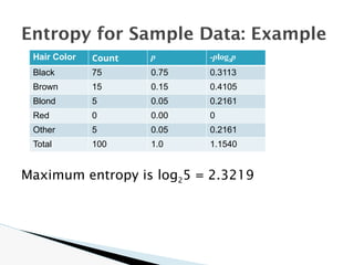
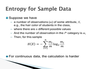
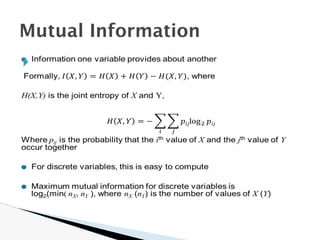
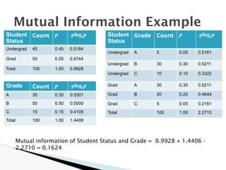
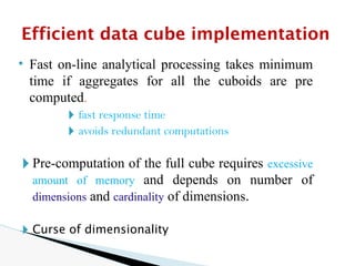
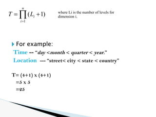
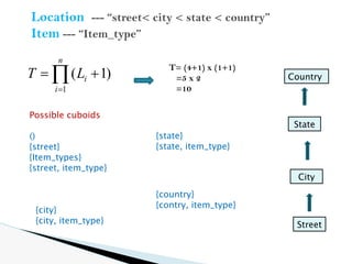
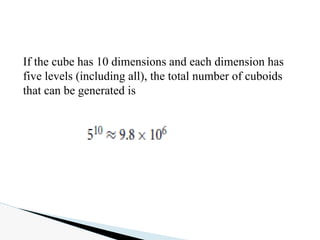
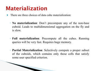
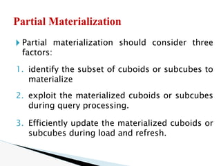
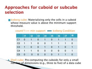
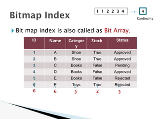
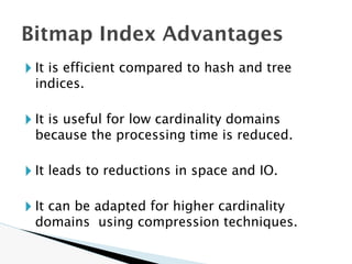
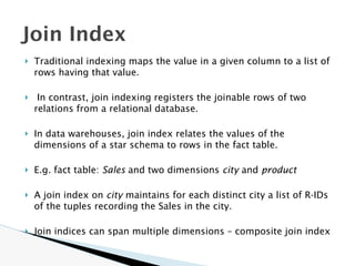
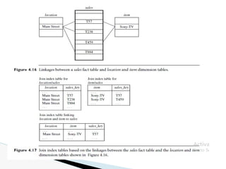
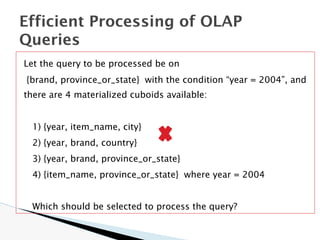
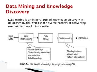
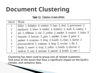
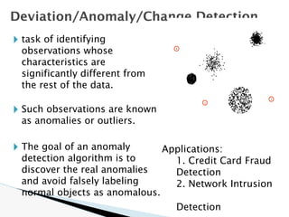
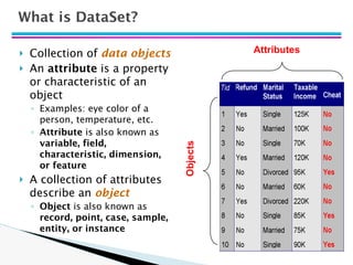
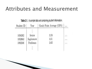
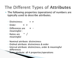
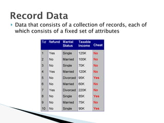
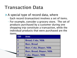
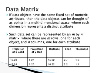
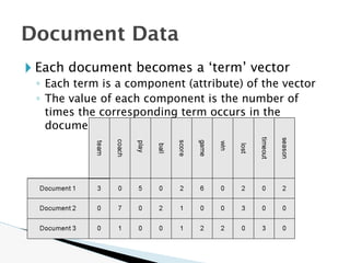
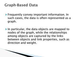
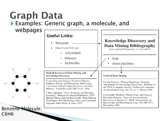
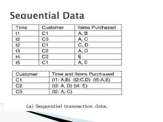
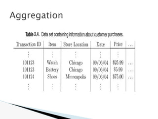
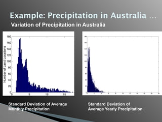
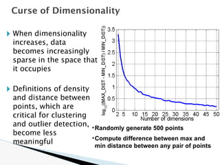
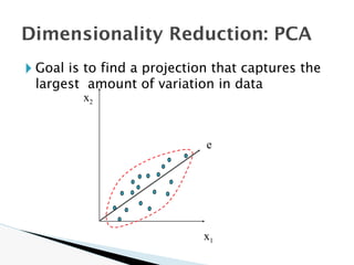
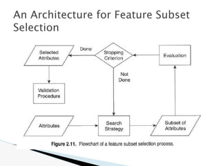
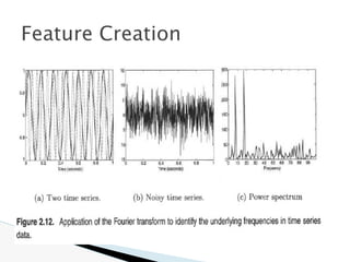
The document discusses data warehouse implementation and efficient data cube computation for OLAP, detailing methods of query processing, cube materialization strategies, and indexing techniques such as bitmap and join indices. It also explores data mining processes, challenges, and tasks, emphasizing the need for scalability, handling high-dimensional data, and employing predictive modeling and clustering techniques to uncover hidden patterns within large datasets. Overall, it highlights the significance of efficient data management in analytics to derive meaningful insights from complex information systems.

1. Data Warehouse
Implementation & Data Mining

2. 🞂 How to compute data cube efficiently
🞂 How OLAP data can be indexed, using either
bitmap or join indices
🞂 How OLAP queries are processed
🞂 Various types of warehouse servers for OLAP
processing
Contents

3. 🞂 You would like to create a data cube
All_Electronics that contains the following:
item, city, year, and sales_in_Euro
🞂 Answer following queries
◦ Compute the sum of sales, grouping by item and
city
◦ Compute the sum of sales, grouping by item
◦ Compute the sum of sales, grouping by city
Data Cube Computation

4. 🞂 Dimension: city, item,year
🞂 The total number of data cuboids is 23
=8
{(city,item,year),
(city,item), (city,year),
(city),(item),(year),
()}
🞂 (), the dimensions are not grouped
◦ These group-by’s form a lattice of cuboids for the data cube
◦ The basic cuboid contains all three dimensions
Data Cube Computation

6. 🞂 An SQL query containing no group-by (e.g., “compute the sum
of total sales”) is a zero dimensional operation.
🞂 An SQL query containing one group-by (e.g., “compute the
sum of sales, group-by city”) is a one-dimensional operation.
🞂 On n dimensions is equivalent to a collection of group-by
statements, one for each subset of the n dimensions.
Data Cube Operator
Data Cube Computation

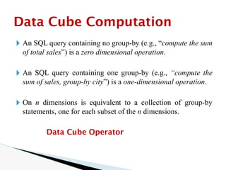
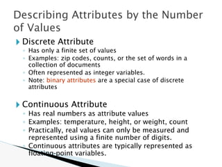
7. 🞂 The compute cube operator computes aggregates
over all subsets of the dimensions specified in the
operation.
🞂 SQL syntax, the data cube could be defined in
DMQL as:
define cube sales [item, city, year]: sum (sales_in_dollars)
🞂 Compute the sales aggregate cuboids as:
compute cube sales
Data Cube Computation

8. A Data Cube: sales
10 11 12 3 10 1
11 9 6 9 6 7
12 9 8 5 7 3
I1 I2 I3
New York
Chicago
Toronto
47
48
44
Al
l
46 37 36 22 29 14 184
Al
l
Cit
y
Item
Aggregate cell Base cell Apex Cuboid
Item cuboid
City cuboid
Base cuboid
Vancouver
I5 I6
I4
5
8 10
13 6 3 45

10. A 3D Data Cube

11. • Fast on-line analytical processing takes minimum
time if aggregates for all the cuboids are pre
computed.
🞂 fast response time
🞂 avoids redundant computations
🞂 Pre-computation of the full cube requires excessive
amount of memory and depends on number of
dimensions and cardinality of dimensions.
🞂 Curse of dimensionality
Efficient data cube implementation

12. 🞂 The storage requirements are even more excessive
when many of the dimensions have associated concept
hierarchies, each with multiple levels.
🞂 This problem is referred to as the curse of
dimensionality.
Efficient data cube implementation

13. 🞂
Efficient data cube implementation

14. 🞂 The total number of cuboids that can be generated is
where Li is the number of levels for dimension i.
Efficient data cube implementation

15. 🞂 For example:
Time -- “day <month < quarter < year.”
Location --- “street< city < state < country”
T= (4+1) x (4+1)
=5 x 5
=25
where Li is the number of levels for
dimension i.

16. Location --- “street< city < state < country”
Item --- “Item_type”
Possible cuboids
()
{street}
{Item_types}
{street, item_type}
Street
City
State
Country
{city}
{city, item_type}
{state}
{state, item_type}
{country}
{contry, item_type}
T= (4+1) x (1+1)
=5 x 2
=10

17. If the cube has 10 dimensions and each dimension has
five levels (including all), the total number of cuboids
that can be generated is

18. 🞂 There are three choices of data cube materialization:
◦ No materialization: Don’t precompute any of the non-base
cuboid. Leads to multidimensional aggregation on the fly and
is slow.
◦ Full materialization: Precompute all the cubes. Running
queries will be very fast. Requires huge memory.
◦ Partial Materialization: Selectively compute a proper subset
of the cuboids, which contains only those cells that satisfy
some user specified criterion.
Materialization

19. 🞂 Partial materialization should consider three
factors:
1. identify the subset of cuboids or subcubes to
materialize
2. exploit the materialized cuboids or subcubes
during query processing.
3. Efficiently update the materialized cuboids or
subcubes during load and refresh.
Partial Materialization

20. Approaches for cuboid or subcube
selection
■Iceberg cube: Materializing only the cells in a cuboid
whose measure value is above the minimum support
threshold.
count(*) >= min support Iceberg Condition
🞂 Shell cube: Pre-computing the cuboids for only a small
number of dimensions (e.g., three to five) of a data cube
I1 I2 I3 I4 I5 I6 I7 I8
C1 0 1 0 1 0 1 1 0
C2 1 1 0 0 1 1 1 0
C3 1 0 0 1 0 1 0 1
C4 1 1 0 0 0 0 0 1
C5 0 0 0 0 0 1 1 0

21. 🞂Bitmap Index
🞂Join Index
Indexing OLAP Data

22. 🞂 Bit map index is also called as Bit Array.
Bitmap Index
ID Name Categor
y
Stock Status
1 A Shoe True Approved
2 B Shoe True Approved
3 C Books False Pending
4 D Books False Approved
5 E Books False Rejected
6 F Toys True Rejected
1 1 2 2 3 4 4
6 3 2 3
6
Cardinality

23. Approved Pending Rejected
1 0 0 0
2 0 0 0
3 0 0 0
4 0 0 0
5 0 0 0
6 0 0 0
ID Name Category Stock Status
1 A Shoe True Approved
2 B Shoe True Approved
3 C Books False Pending
4 D Books False Approved
5 E Books False Rejected
6 F Toys True Rejected

24. Approved Pending Rejected
1 1 0 0
2 1 0 0
3 0 1 0
4 1 0 0
5 0 0 1
6 0 0 1
ID Name Category Stock Status
1 A Shoe True Approved
2 B Shoe True Approved
3 C Books False Pending
4 D Books False Approved
5 E Books False Rejected
6 F Toys True Rejected
1 2 4
1 2 3 4

25. 🞂 Bitmap Index is popular in OLAP products because it allows
quick searching in data cubes.
🞂 In the bitmap index for a given attribute, there is a distinct
bit vector, Bv, for each value v in the attribute’s domain.
🞂 If a given attribute’s domain consists of n values, then n bits
are needed for each entry in the bitmap index (i.e., there are
n bit vectors).
🞂 If the attribute has the value v for a given row in the data
table, then the bit representing that value is set to 1 in the
corresponding row of the bitmap index. All other bits for that
row are set to 0.
Bitmap Index

27. 🞂 It is efficient compared to hash and tree
indices.
🞂 It is useful for low cardinality domains
because the processing time is reduced.
🞂 It leads to reductions in space and IO.
🞂 It can be adapted for higher cardinality
domains using compression techniques.
Bitmap Index Advantages

28. 🞂 Traditional indexing maps the value in a given column to a list of
rows having that value.
🞂 In contrast, join indexing registers the joinable rows of two
relations from a relational database.
🞂 In data warehouses, join index relates the values of the
dimensions of a star schema to rows in the fact table.
🞂 E.g. fact table: Sales and two dimensions city and product
🞂 A join index on city maintains for each distinct city a list of R-IDs
of the tuples recording the Sales in the city.
🞂 Join indices can span multiple dimensions – composite join index
Join Index

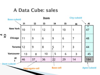
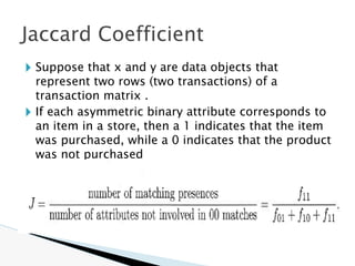
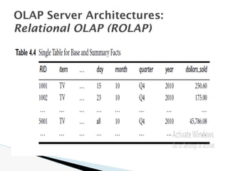
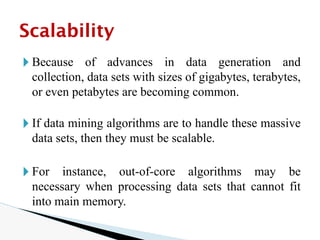
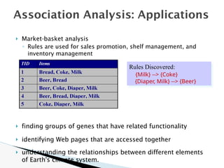
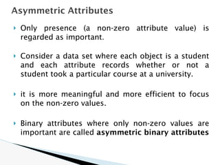
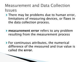
30. 1. Determine which operations should be performed on the available
cuboids
e.g., dice = selection + projection
2. Determine which materialized cuboid(s) should be selected for
OLAP operation.
◦ the one with low cost
Suppose that we define a data cube for AllElectronics of the form
“sales cube [time, item, location]: sum(sales in dollars).”
The dimension hierarchies used are
“day < month < quarter < year” for time;
“item name < brand < type” for item;
“street < city < province or state < country” for location.
Efficient Processing of OLAP
Queries

31. Let the query to be processed be on
{brand, province_or_state} with the condition “year = 2004”, and
there are 4 materialized cuboids available:
1) {year, item_name, city}
2) {year, brand, country}
3) {year, brand, province_or_state}
4) {item_name, province_or_state} where year = 2004
Which should be selected to process the query?
Efficient Processing of OLAP
Queries

32. 🞂 ROLAP
🞂 MOLAP
🞂 HOLAP
OLAP Server Architectures

33. 🞂 ROLAP works directly with relational databases.
🞂 Uses a relational or extended-relational DBMS to store and manage
warehouse data.
🞂 ROLAP tools do not use pre-calculated data cubes but instead pose
the query to the standard relational database.
🞂 ROLAP tools feature the ability to ask any question because the
methodology does not limit to the contents of a cube.
🞂 ROLAP also has the ability to drill down to the lowest level of
detail in the database.
🞂 optimization for each DBMS, implementation of aggregation
navigation logic, and additional tools and services
Relational OLAP (ROLAP)

34. OLAP Server Architectures:
Relational OLAP (ROLAP)

35. 🞂 MOLAP stores this data in an optimized multi-dimensional array storage.
🞂 The advantage of using a data cube is that it allows fast indexing to pre-
computed summarized data.
🞂 MOLAP tools have a very fast response time.
🞂 The data cube contains all the possible answers to a given range of
questions.
🞂 MOLAP servers adopt a two-level storage representation to handle dense
and sparse data sets.
🞂 Sparse subcubes employ compression technology for efficient storage
utilization
Multidimensional OLAP (MOLAP)

37. 🞂 HOLAP server may allow large volumes of detailed data to be stored
in a relational database
🞂 Aggregations are kept in a separate MOLAP store.
🞂 HOLAP tools can utilize both pre-calculated cubes and relational data
sources.
🞂 The hybrid OLAP approach combines ROLAP and MOLAP
technology, benefiting from the greater scalability of ROLAP and the
faster computation of MOLAP.
🞂 The Microsoft SQL Server 2000 supports a hybrid OLAP server.
Hybrid OLAP (HOLAP)

38. Data Mining

39. ▪What is data mining?
▪Challenges
▪Data Mining Tasks
▪Data: Types of Data
▪Data Quality
▪Data Preprocessing
▪Measures of Similarity and Dissimilarity
Contents

40. 🞂 Data mining is the process of automatically discovering useful
information in large data repositories.
🞂 Finding hidden information in a database.
🞂 Data mining techniques are deployed to scour large databases
in order to find novel and useful patterns that might otherwise
remain unknown.
🞂 They also provide capabilities to predict the outcome of a
future observation.
What Is Data Mining?( Definition)

41. 🞂 Looking up individual records using a database
management system.
🞂 finding particular Web pages via a query to an
Internet search engine.
🞂 Above are tasks related to the area of information
retrieval.
What is (not) Data Mining?

42. Data Mining and Knowledge
Discovery
Data mining is an integral part of knowledge discovery in
databases (KDD), which is the overall process of converting
raw data into useful information,

43. 🞂 The input data can be stored in a variety of
formats.
🞂 To transform the raw input data into an
appropriate format for subsequent analysis.
🞂 It includes:
▪Fusing data from multiple sources
▪cleaning data to remove noise and duplicate
observations
▪selecting records and features that are
relevant to the data mining task at hand.
Data Preprocessing

44. 🞂 Ensures that only valid and useful results are
incorporated into the DSS.
🞂 Which allows analysts to explore the data and
the data mining results from a variety of
viewpoints.
🞂 Testing methods can also be applied during
post processing to eliminate spurious data
mining results.
Post processing

45. 🞂 Scalability
🞂 High Dimensionality
🞂 Heterogeneous and Complex Data
🞂 Data Ownership and Distribution
🞂 Non-traditional Analysis
Challenges -motivated the
development of data mining

46. 🞂 Because of advances in data generation and
collection, data sets with sizes of gigabytes, terabytes,
or even petabytes are becoming common.
🞂 If data mining algorithms are to handle these massive
data sets, then they must be scalable.
🞂 For instance, out-of-core algorithms may be
necessary when processing data sets that cannot fit
into main memory.
Scalability

47. 🞂 It is now common to encounter data sets with hundreds or thousands of
attributes instead of the handful common a few decades ago.
🞂 For example,
consider a data set that contains measurements of temperature a various
locations.
🞂 Traditional data analysis techniques that were developed for low-
dimensional data often do not work well for such high dimensional data.
🞂 Also, for some data analysis algorithms, the computational complexity
increases rapidly as the dimensionality (the number of features) increases.
High Dimensionality

48. 🞂 As the role of data mining in business, science,
medicine, and other fields has grown, so has the need
for techniques that can handle heterogeneous attributes.
🞂 Recent years have also seen the emergence of more
complex data objects.
🞂 Techniques developed for mining such complex objects
should take into consideration relationships in the data
Heterogeneous and Complex Data

49. 🞂 Sometimes, the data needed for an analysis is not stored in one location
or owned by one organization. Instead, the data is geographically
distributed among resources belonging to multiple entities.
🞂 This requires the development of distributed data mining techniques.
🞂 Among the key challenges faced by distributed data mining algorithms
include
1. how to reduce the amount of communication needed to perform the
distributed computation
2. how to effectively consolidate the data mining results obtained from
multiple sources, and
3. how to address data security issues.
Data ownership and Distribution

50. 🞂 The traditional statistical approach is based on a hypothesize-
and-test paradigm. This process is extremely labor-intensive.
🞂 Current data analysis tasks often require the generation and
evaluation of thousands of hypotheses
🞂 consequently, the development of some data mining
techniques has been motivated by the desire to automate the
process of hypothesis generation and evaluation.
Non-traditional Analysis

51. 🞂 Predictive tasks: Predict the value of a
particular attribute based on the values of
other attributes.
◦ Target or dependent variable
◦ Explanatory or independent variables.
🞂 Descriptive tasks: Derive patterns that
summarize the underlying relationships in
data.
◦ Post-processing techniques are used to validate and
explain the result.
Data Mining Tasks

52. Predictive Modeling
Clustering
Association
Rules
Anomaly
Detection
Milk
Data
Data Mining Tasks …

53. 🞂 Refers to the task of building a model for the target
variable as the function of the explanatory variables.
🞂 There are two types of predictive modeling tasks:
▪classification: which is used for discrete target variables.
▪regression, which is used for continuous target variables.
🞂 Example predicting whether a web user will make a
purchase at an online book store.
🞂 forecasting the future price of the stock.
Predictive Modeling

54. 🞂 Consider the task of predicting a species of flower
based on the characteristics of the flower
🞂 Consider classifying an Iris flower as to whether it
belongs to one of the following three Iris species:
Setosa, Versicolour, or Virginica.
🞂 Data set contains four other attributes: sepal width,
sepal length, petal length, and petal width.
Example

56. 🞂 Petal width is broken into the categories low, medium,
and high, which correspond to the intervals [0' 0.75),
[0.75, 1.75), [1.75, ∞), respectively.
🞂 Also, petal length is broken into categories low,
medium, and high, which correspond to the intervals
[0, 2.5), [2.5,5), [5, ∞), respectively

57. Based on these categories of petal width and
length, the following rules can be derived:
oPetal width low and petal length low implies Setosa.
oPetal width medium and petal length medium implies
Versicolour.
oPetal width high and petal length high implies
Virginica.

58. 🞂 Given a set of records each of which contain
some number of items from a given collection
🞂 used to discover patterns that describe
strongly associated features in the data.
🞂 The discovered patterns are typically
represented in the form of implication rules
or feature subsets
Association Analysis: Definition

59. 🞂 Market-basket analysis
◦ Rules are used for sales promotion, shelf management, and
inventory management
🞂 finding groups of genes that have related functionality
🞂 identifying Web pages that are accessed together
🞂 understanding the relationships between different elements
of Earth's climate system.
Association Analysis: Applications
Rules Discovered:
{Milk} --> {Coke}
{Diaper, Milk} --> {Beer}

60. 🞂 Finding groups of objects such that the objects
in a group will be similar (or related) to one
another and different from (or unrelated to) the
objects in other groups
Inter-cluster
distances are
maximized
Intra-cluster
distances are
minimized
Cluster Analysis

61. Document Clustering
Clustering has been used to group sets of related customers
find areas of the ocean that have a significant impact on the Earth's
climate, and compress data.

62. 🞂 task of identifying
observations whose
characteristics are
significantly different from
the rest of the data.
🞂 Such observations are known
as anomalies or outliers.
🞂 The goal of an anomaly
detection algorithm is to
discover the real anomalies
and avoid falsely labeling
normal objects as anomalous.
Deviation/Anomaly/Change Detection
Applications:
1. Credit Card Fraud
Detection
2. Network Intrusion
Detection

63. What is DataSet?
🞂 Collection of data objects
🞂 An attribute is a property
or characteristic of an
object
◦ Examples: eye color of a
person, temperature, etc.
◦ Attribute is also known as
variable, field,
characteristic, dimension,
or feature
🞂 A collection of attributes
describe an object
◦ Object is also known as
record, point, case, sample,
entity, or instance
Attributes
Objects

64. Attributes and Measurement

65. Attributes and Measurement
🞂 An attribute is a property or characteristic of an
object that may vary; either from one object to
another or from one time to another.
🞂 Ex: eye color varies from person to person, while the
temperature of an object varies over time
🞂 Note that eye color is a symbolic attribute with a
small number of possible values {brown,black,blue,
green,hazel, etc.}
🞂 while temperature is a numerical attribute with a
potentially unlimited number of values.

66. Attributes and Measurement
🞂 A measurement scale is a rule (function)
that associates a numerical or symbolic
value with an attribute of an object.
🞂 The process of measurement is the
application of a measurement scale to
associate a value with a particular attribute of
a specific object

67. 🞂 The values used to represent an attribute may
have properties that are not properties of the
attribute itself, and vice versa
🞂 Distinction between attributes and attribute values
◦ Same attribute can be mapped to different attribute
values
● Example: height can be measured in feet or meters
◦ Different attributes can be mapped to the same set of
values
● Example: Attribute values for ID and age are integers
● But properties of attribute values can be different
● ID has no limit but age has a maximum and minimum value
Type of an Attribute

68. Measurement of Length
● The way you measure an attribute may not match the
attributes properties.
This scale
preserves
the ordering
and additvity
properties of
length.
This scale
preserves
only the
ordering
property of
length.

69. 🞂 The following properties (operations) of numbers are
typically used to describe attributes.
◦ Distinctness: = ≠
◦ Order: < >
◦ Differences are + -
meaningful :
◦ Ratios are * /
meaningful
◦ Nominal attribute: distinctness
◦ Ordinal attribute: distinctness & order
◦ Interval attribute: distinctness, order & meaningful
differences
◦ Ratio attribute: all 4 properties/operations
The Different Types of Attributes

70. 🞂 There are different types of attributes
◦ Nominal
● Examples: ID numbers, eye color, zip codes
◦ Ordinal
● Examples: rankings (e.g., place in competition),
grades, height {tall, medium, short}
◦ Interval
● Examples: calendar dates, temperatures in Celsius
or Fahrenheit.
◦ Ratio
● Examples: height, weight, length, time, counts
Types of Attributes

71. Different Attributes types

72. Permissible Transformation that do not change the
attributes meaning

73. 🞂 Discrete Attribute
◦ Has only a finite set of values
◦ Examples: zip codes, counts, or the set of words in a
collection of documents
◦ Often represented as integer variables.
◦ Note: binary attributes are a special case of discrete
attributes
🞂 Continuous Attribute
◦ Has real numbers as attribute values
◦ Examples: temperature, height, or weight, count
◦ Practically, real values can only be measured and
represented using a finite number of digits.
◦ Continuous attributes are typically represented as
floating-point variables.
Describing Attributes by the Number
of Values

74. Asymmetric Attributes
🞂 Only presence (a non-zero attribute value) is
regarded as important.
🞂 Consider a data set where each object is a student
and each attribute records whether or not a
student took a particular course at a university.
🞂 it is more meaningful and more efficient to focus
on the non-zero values.
🞂 Binary attributes where only non-zero values are
important are called asymmetric binary attributes

75. ◦ Dimensionality (number of attributes)
●Less dimension may not lead to qualitative mining results
● High dimensional data –Curse of dimensionality
●an important motivation in preprocessing the data is
dimensionality reduction.
◦ Sparsity
●only the non-zero values need to be stored and manipulated which
improves computation time and storage.
◦ Resolution
●obtain data at different levels of resolution, and often the properties
of the data are different at different resolution.
●Patterns should not be too fine or too coarse, it would not be visible.
Important Characteristics of Data Set

76. 🞂 Record
◦ Data Matrix
◦ Document Data
◦ Transaction Data
🞂 Graph
◦ World Wide Web
◦ Molecular Structures
🞂 Ordered
◦ Spatial Data
◦ Temporal Data
◦ Sequential Data
◦ Genetic Sequence Data
Types of data sets

77. 🞂 Data that consists of a collection of records, each of
which consists of a fixed set of attributes
Record Data

78. 🞂 A special type of record data, where
◦ Each record (transaction) involves a set of items.
◦ For example, consider a grocery store. The set of
products purchased by a customer during one
shopping trip constitute a transaction, while the
individual products that were purchased are the
items.
Transaction Data

79. 🞂 If data objects have the same fixed set of numeric
attributes, then the data objects can be thought of
as points in a multi-dimensional space, where each
dimension represents a distinct attribute
🞂 Such data set can be represented by an m by n
matrix, where there are m rows, one for each
object, and n columns, one for each attribute
Data Matrix

80. 🞂 A sparse data matrix is a special case of a
data matrix in which the attributes are of the
same type and are asymmetric
🞂 only non-zero values are important.
🞂 Transaction data is an example of a sparse
data matrix that has only 0 1 entries.
🞂 Another common example is document data.
The Sparse Data Matrix

81. 🞂 Each document becomes a ‘term’ vector
◦ Each term is a component (attribute) of the vector
◦ The value of each component is the number of
times the corresponding term occurs in the
document.
Document Data

82. 🞂 Frequently convey important information. In
such cases, the data is often represented as a
graph.
🞂 In particular, the data objects are mapped to
nodes of the graph, while the relationships
among objects are captured by the links
between objects and link properties, such as
direction and weight.
Graph-Based Data

83. 🞂 Examples: Generic graph, a molecule, and
webpages
Graph Data
Benzene Molecule:
C6H6

84. 🞂 For some types of data, the attributes have
relationships that involve order in time or
space
🞂 Different types of ordered data are
◦ Sequential Data
◦ Sequence Data
◦ Time Series Data
◦ Spatial Data
Ordered Data

85. Sequential Data
Items/Eents

86. Genomic sequence data

87. Time Series Data

88. Spatial Data
Average Monthly
Temperature of
land and ocean
Spatio-Temporal Data

89. 🞂 Data mining focuses on
(1) the detection and correction of data quality
Problems - Data cleaning
(2) the use of robust algorithms that can tolerate
poor data quality.
Data Quality

90. 🞂 There may be problems due to human error,
limitations of measuring devices, or flaws in
the data collection process.
🞂 measurement error refers to any problem
resulting from the measurement process
🞂 For continuous attributes, the numerical
difference of the measured and true value is
called the error.
Measurement and Data Collection
Issues

91. 🞂 The term data collection error refers to errors
such as :
1. missing values or even entire data objects may
be.
2. There may be spurious or duplicate objects
🞂 Examples of data quality problems:
◦ Noise and outliers
◦ Missing values
◦ Duplicate data
◦ Wrong data
Measurement and Data Collection
Issues

92. 🞂 Noise is the random component of a
measurement error.
🞂 It may involve the distortion of a value or the
addition of spurious objects.
Noise

94. 🞂 Data errors may be the result of a more
deterministic phenomenon, such as a streak
in the same place on a set of photographs.
🞂 Such deterministic distortions of the data are
often referred to as artifacts.
Artifacts

95. 🞂 The closeness of repeated measurements( of
the same quantity) to one another.
🞂 A systematic variation of the measurements
from the quantity being measured.
🞂 The closeness of measurements to the true
value of the quantity being measured.
Precision, Bias, and Accuracy

96. 🞂 Outliers are data objects with characteristics
that are considerably different than most of
the other data objects in the data set
◦ Case 1: Outliers are
noise that interferes
with data analysis
◦ Case 2: Outliers are
the goal of our analysis
● Credit card fraud
● Intrusion detection
Outliers

97. 🞂 Reasons for missing values
◦ Information is not collected
(e.g., people decline to give their age and weight)
◦ Attributes may not be applicable to all cases
(e.g., annual income is not applicable to children)
🞂 Handling missing values
◦ Eliminate data objects or variables
◦ Estimate missing values
●Example: time series of temperature
◦ Ignore the missing value during analysis
●Inconsistent
●Duplicate
Missing Values

98. 🞂 Data set may include data objects that are
duplicates, or almost duplicates of one
another
◦ Major issue when merging data from
heterogeneous sources
🞂 Examples:
◦ Same person with multiple email addresses
◦ Two distinct persons with same name
Duplicate Data

99. 🞂 Timeliness
🞂 Relevance
🞂 Knowledge about the Data
Data quality Issues Related to
Applications

100. 🞂 Aggregation
🞂 Sampling
🞂 Dimensionality reduction
🞂 Feature subset selection
🞂 Feature creation
🞂 Discretization and binarization
🞂 Variable transformation
Data Preprocessing

101. ● Combining two or more attributes (or objects) into a
single attribute (or object)
● Purpose
– Data reduction
◆ Reduce the number of attributes or objects
– Change of scale
◆ Cities aggregated into regions, states, countries, etc.
◆ Days aggregated into weeks, months, or years
– More “stable” data
◆ Aggregated data tends to have less variability
Aggregation

102. Aggregation

103. Example: Precipitation in Australia …
Standard Deviation of Average
Monthly Precipitation
Standard Deviation of
Average Yearly Precipitation
Variation of Precipitation in Australia

104. Sampling
🞂 Sampling is the main technique employed for
data reduction.
◦ It is often used for both the preliminary investigation
of the data and the final data analysis.
🞂 Statisticians often sample because obtaining
the entire set of data of interest is too
expensive or time consuming.
🞂 Sampling is typically used in data mining
because processing the entire set of data of
interest is too expensive or time consuming.

105. Sampling …
🞂 The key principle for effective sampling is the
following:
◦ Using a sample will work almost as well as using
the entire data set, if the sample is representative
◦ A sample is representative if it has approximately
the same properties (of interest) as the original set
of data

106. Sample Size
8000 points 2000 Points 500 Points

107. Types of Sampling
🞂 Simple Random Sampling
◦ There is an equal probability of selecting any particular
item
◦ Sampling without replacement
●As each item is selected, it is removed from the
population
◦ Sampling with replacement
●Objects are not removed from the population as they
are selected for the sample.
●In sampling with replacement, the same object can
be picked up more than once
🞂 Stratified sampling
◦ Split the data into several partitions; then draw random
samples from each partition
🞂 Progressive sampling

108. Sample Size
🞂 What sample size is necessary to get at least one
object from each of 10 equal-sized groups.

109. Dimensionality Reduction
🞂 Purpose:
◦ Avoid curse of dimensionality
◦ Reduce amount of time and memory required by
data mining algorithms
◦ Allow data to be more easily visualized
◦ May help to eliminate irrelevant features or reduce
noise
🞂 Techniques
◦ Principal Components Analysis (PCA)
◦ Singular Value Decomposition
◦ Others: supervised and non-linear techniques

110. Curse of Dimensionality
🞂 When dimensionality
increases, data
becomes increasingly
sparse in the space that
it occupies
🞂 Definitions of density
and distance between
points, which are
critical for clustering
and outlier detection,
become less
meaningful
•Randomly generate 500 points
•Compute difference between max and
min distance between any pair of points

111. Dimensionality Reduction: PCA
🞂 Goal is to find a projection that captures the
largest amount of variation in data
x2
x1
e

112. Feature Subset Selection
🞂 Another way to reduce dimensionality of data
🞂 Redundant features
◦ Duplicate much or all of the information contained
in one or more other attributes
◦ Example: purchase price of a product and the
amount of sales tax paid
🞂 Irrelevant features
◦ Contain no information that is useful for the data
mining task at hand
◦ Example: students' ID is often irrelevant to the task
of predicting students' GPA

113. 🞂 Embedded approaches
🞂 Filter approaches
🞂 Wrapper approaches
Feature Subset Selection

114. An Architecture for Feature Subset
Selection

115. 🞂 High
🞂 Low
Feature Weighting

116. Feature Creation

117. 🞂 Feature Extraction
🞂 Mapping the Data to a New Space
🞂 Fourier transform

118. Discretization Without Using Class
Labels
Equal interval width approach used to obtain 4 values.

119. Discretization Without Using Class
Labels
Equal frequency approach used to obtain 4 values.

120. Discretization Without Using Class Labels
K-means approach to obtain 4 values.

121. Binarization

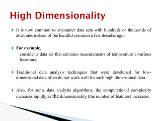
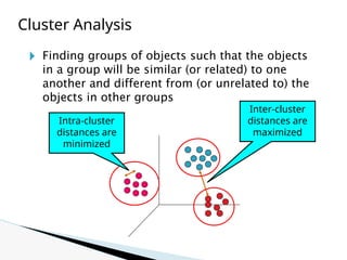
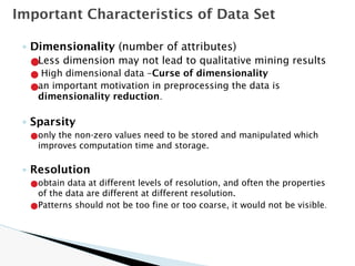
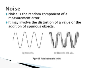
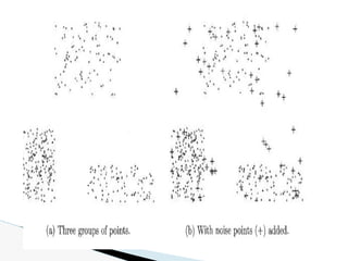
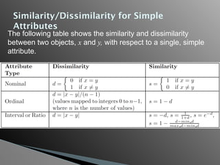
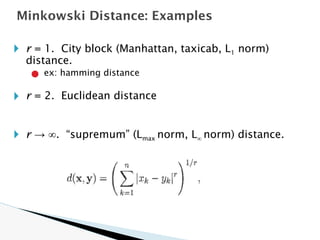
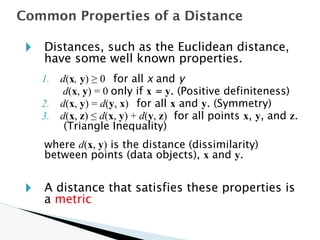
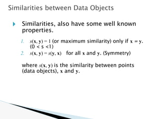
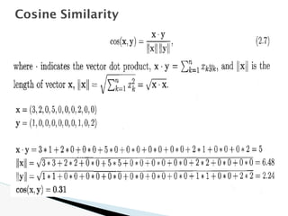
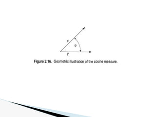
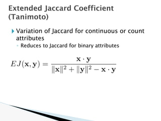
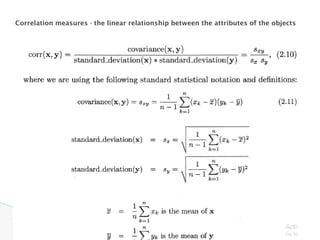
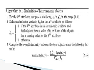
122. 🞂 Similarity measure
◦ Numerical measure of how alike two data objects are.
◦ Is higher when objects are more alike.
◦ Often falls in the range [0,1]
🞂 Dissimilarity measure
◦ Numerical measure of how different two data objects are
◦ Lower when objects are more alike
◦ Minimum dissimilarity is often 0
◦ Upper limit varies
🞂 Proximity refers to a similarity or dissimilarity
Similarity and Dissimilarity
Measures

123. Similarity/Dissimilarity for Simple
Attributes
The following table shows the similarity and dissimilarity
between two objects, x and y, with respect to a single, simple
attribute.

124. Dissimilarities between Data Objects - Distance
🞂 Euclidean Distance
where n is the number of dimensions (attributes)
and xk and yk are, respectively, the kth
attributes
(components) or data objects x and y.

125. 🞂 Minkowski Distance is a generalization of
Euclidean Distance
Where r is a parameter, n is the number
of dimensions (attributes) and xk and yk
are, respectively, the kth
attributes
(components) or data objects x and y.
Minkowski Distance

126. Euclidean Distance

128. 🞂 r = 1. City block (Manhattan, taxicab, L1 norm)
distance.
● ex: hamming distance
🞂 r = 2. Euclidean distance
🞂 r → ∞. “supremum” (Lmax norm, L∞ norm) distance.
Minkowski Distance: Examples

129. 🞂 Distances, such as the Euclidean distance,
have some well known properties.
1. d(x, y) ≥ 0 for all x and y
d(x, y) = 0 only if x = y. (Positive definiteness)
2. d(x, y) = d(y, x) for all x and y. (Symmetry)
3. d(x, z) ≤ d(x, y) + d(y, z) for all points x, y, and z.
(Triangle Inequality)
where d(x, y) is the distance (dissimilarity)
between points (data objects), x and y.
🞂 A distance that satisfies these properties is
a metric
Common Properties of a Distance

130. 🞂 Non-metric Dissimilarities: Set Differences
◦ d(A,B): size(A- B) + size(B - A)
🞂 Non-metric Dissimilarities: Time
Examples

131. 🞂 Similarities, also have some well known
properties.
1. s(x, y) = 1 (or maximum similarity) only if x = y.
(0 < s <1)
2. s(x, y) = s(y, x) for all x and y. (Symmetry)
where s(x, y) is the similarity between points
(data objects), x and y.
Similarities between Data Objects

132. 🞂 Similarity measures between objects that contain only
binary attributes are called similarity coefficients, and
typically have values between 0 and 1.
Let x and y be two objects that consist of n binary attributes.
Similarity Measures for Binary Data
Simple Matching
Coefficient

133. 🞂 Suppose that x and y are data objects that
represent two rows (two transactions) of a
transaction matrix .
🞂 If each asymmetric binary attribute corresponds to
an item in a store, then a 1 indicates that the item
was purchased, while a 0 indicates that the product
was not purchased
Jaccard Coefficient

134. SMC versus Jaccard: Example

135. 🞂
Cosine Similarity

137. 🞂 Variation of Jaccard for continuous or count
attributes
◦ Reduces to Jaccard for binary attributes
Extended Jaccard Coefficient
(Tanimoto)

138. Correlation measures - the linear relationship between the attributes of the objects

139. Visually Evaluating Correlation
Scatter plots
showing the
similarity from
–1 to 1.

140. 🞂 x = (-3, -2, -1, 0, 1, 2, 3)
🞂 y = (9, 4, 1, 0, 1, 4, 9)
yi = xi
2
🞂 mean(x) = 0, mean(y) = 4
🞂 std(x) = 2.16, std(y) = 3.74
🞂 corr = (-3)(5)+(-2)(0)+(-1)(-3)+(0)(-4)+(1)(-3)+(2)(0)+3(5) / ( 6 * 2.16 * 3.74 )
= 0
Drawback of Correlation

141. Bregman Divergence

142. 🞂 A generalization of Euclidean distance
🞂 is useful when attributes are correlated, have
different ranges of values (different
variances), and the distribution of the data is
approximately Gaussian
Mahalanobis distance,

144. 🞂 Domain of application
◦ Similarity measures tend to be specific to the type of attribute
and data
◦ Record data, images, graphs, sequences, 3D-protein structure,
etc. tend to have different measures
🞂 However, one can talk about various properties that
you would like a proximity measure to have
◦ Symmetry is a common one
◦ Tolerance to noise and outliers is another
◦ Ability to find more types of patterns?
◦ Many others possible
🞂 The measure must be applicable to the data and
produce results that agree with domain knowledge
Comparison of Proximity Measures

145. 🞂
Entropy

146. 🞂
Entropy Examples

147. Maximum entropy is log25 = 2.3219
Entropy for Sample Data: Example
Hair Color Count p -plog2p
Black 75 0.75 0.3113
Brown 15 0.15 0.4105
Blond 5 0.05 0.2161
Red 0 0.00 0
Other 5 0.05 0.2161
Total 100 1.0 1.1540

148. 🞂
Entropy for Sample Data

149. 🞂
Mutual Information

150. Mutual Information Example
Student
Status
Count p -plog2p
Undergrad 45 0.45 0.5184
Grad 55 0.55 0.4744
Total 100 1.00 0.9928
Grade Count p -plog2p
A 35 0.35 0.5301
B 50 0.50 0.5000
C 15 0.15 0.4105
Total 100 1.00 1.4406
Student
Status
Grade Count p -plog2p
Undergrad A 5 0.05 0.2161
Undergrad B 30 0.30 0.5211
Undergrad C 10 0.10 0.3322
Grad A 30 0.30 0.5211
Grad B 20 0.20 0.4644
Grad C 5 0.05 0.2161
Total 100 1.00 2.2710
Mutual information of Student Status and Grade = 0.9928 + 1.4406 -
2.2710 = 0.1624

151. 🞂 Applies mutual information to two continuous variables
🞂 Consider the possible binnings of the variables into
discrete categories
◦ nX × nY ≤ N0.6
where
● nX is the number of values of X
● nY is the number of values of Y
● N is the number of samples (observations, data objects)
🞂 Compute the mutual information
◦ Normalized by log2(min( nX, nY )
🞂 Take the highest value
Maximal Information Coefficient