Downloaded 89 times

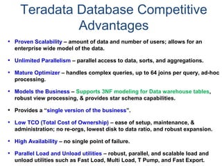
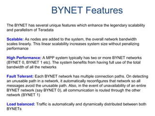

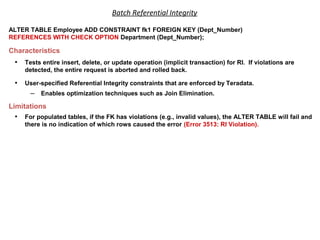
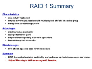
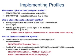
![Partitioning with CASE_N and RANGE_N
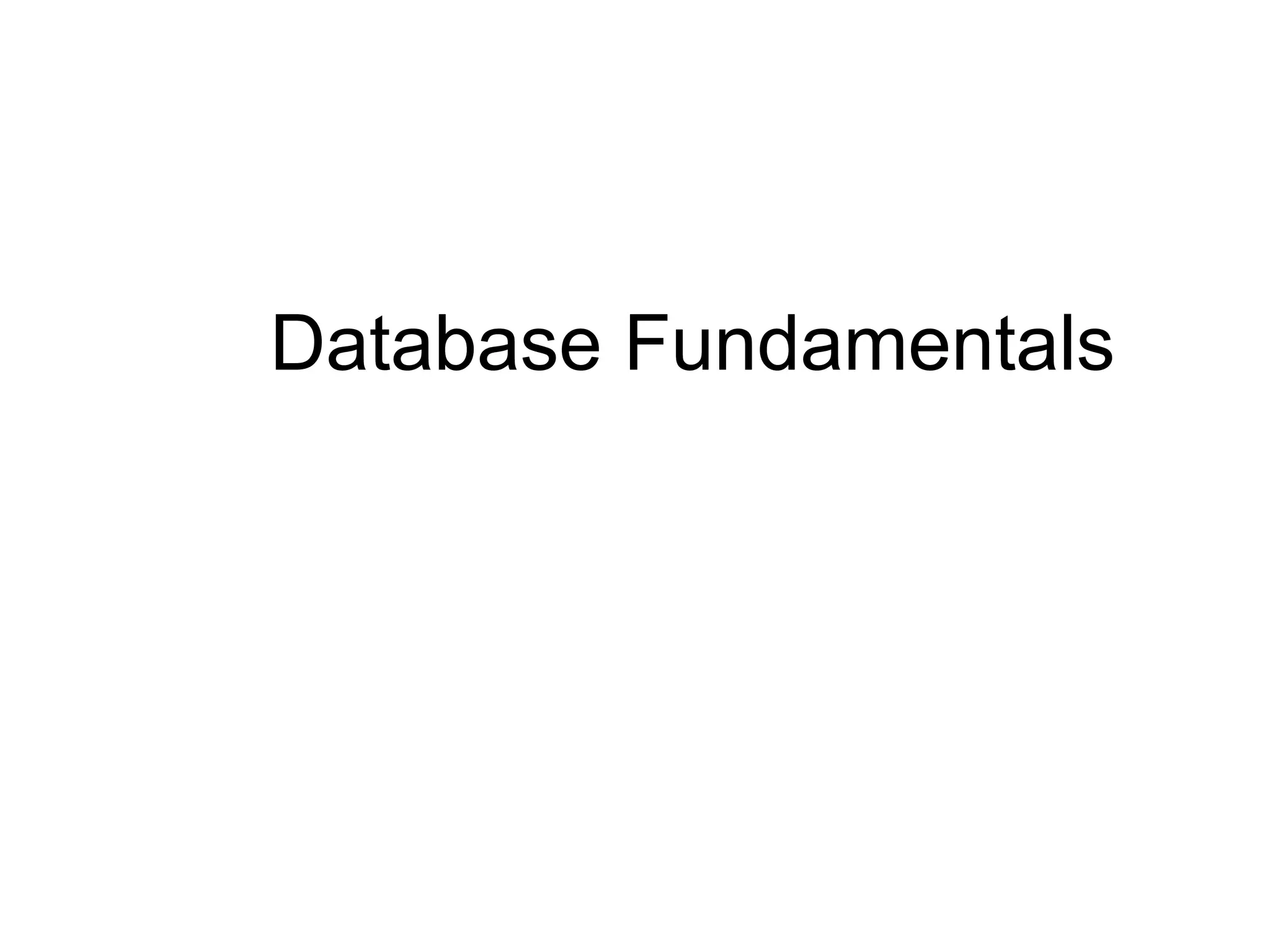
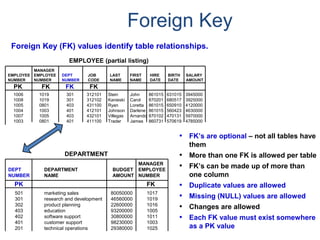
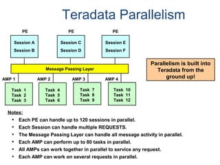
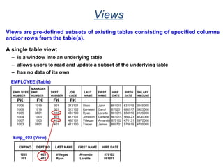
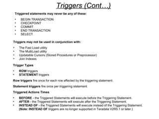
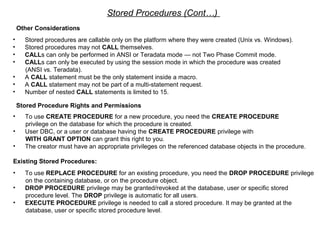
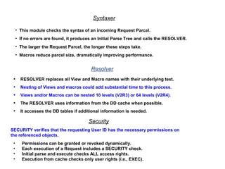
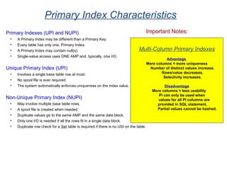
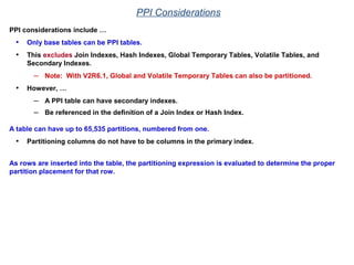
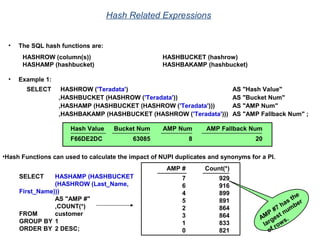
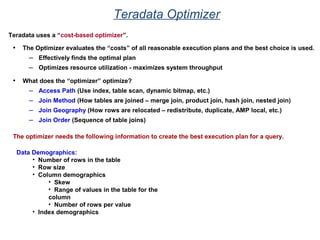
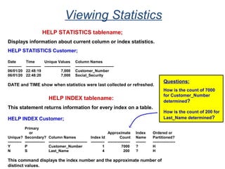
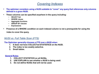
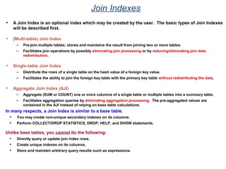
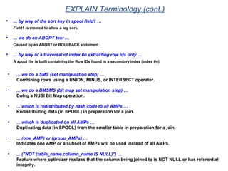
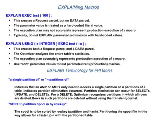
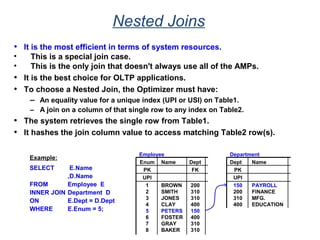
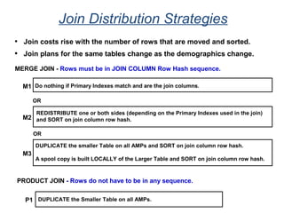
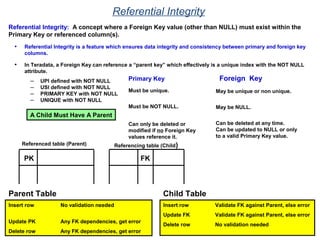
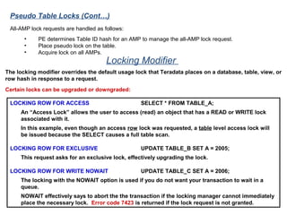
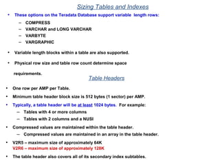
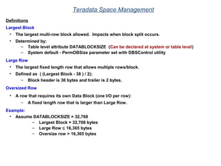
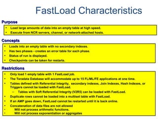
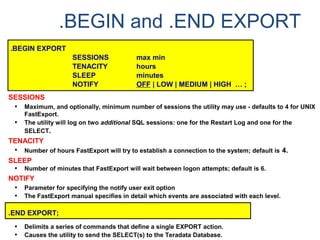
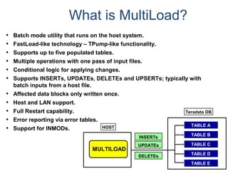
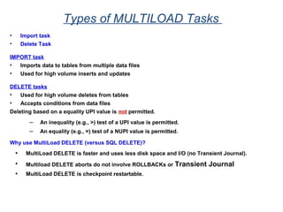
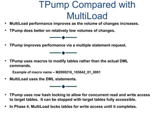
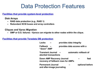
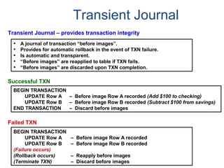
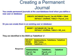
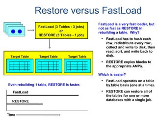
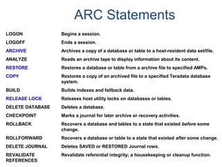
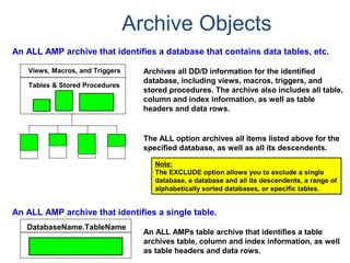
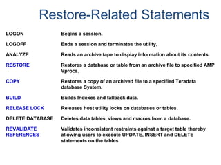
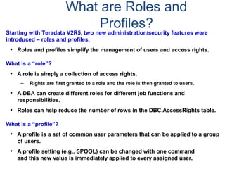
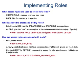
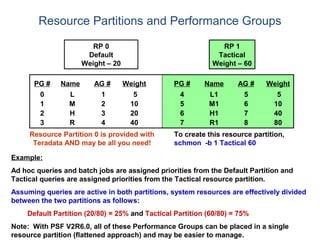
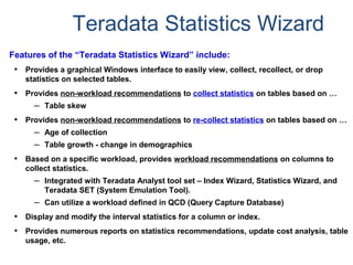
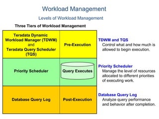
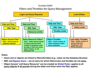
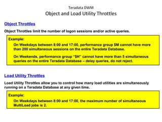
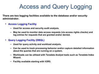
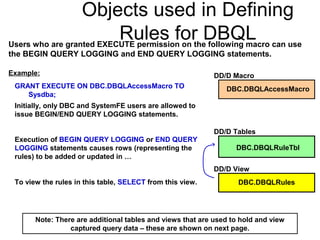
The <partitioning expression> may use one of the following functions to help
define partitions.
• CASE_N
• RANGE_N
Use of CASE_N results in the following:
• Evaluates a list of conditions and returns the position of the first condition that evaluates to
TRUE.
• Result is the data row being placed into a partition associated with that condition.
Use of RANGE_N results in the following:
• The expression is evaluated and is mapped into one of a list of specified ranges.
• Ranges are listed in increasing order and must not overlap with each other.
• Result is the data row being placed into a partition associated with that range.
The PPI keywords used to define two specific-use partitions are:
NO CASE (or NO RANGE) [OR UNKNOWN]
• If this option is used, then a specific-use partition is used when the expression
isn't true for
any case (or is out of range).
• If OR UNKNOWN is included with the NO CASE (or NO RANGE), then UNKNOWN
expressions are also placed in this partition.
UNKNOWN
• If this option is specified, a different specific-use partition is used for unknowns.](https://image.slidesharecdn.com/teradataa-z-160821064323/85/Teradata-a-z-55-320.jpg)
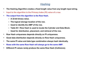
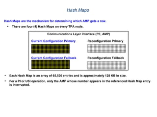
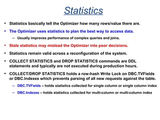
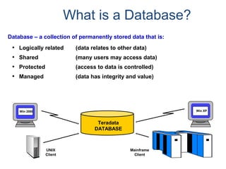
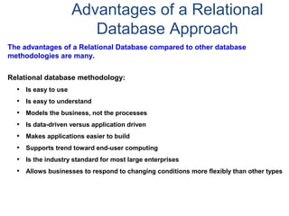
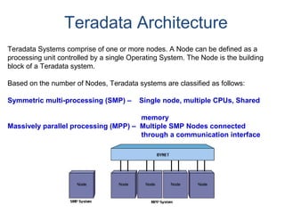
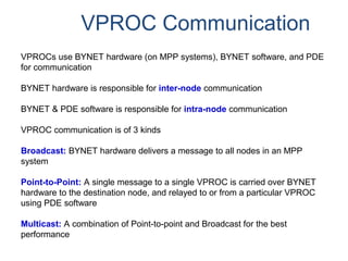
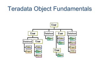
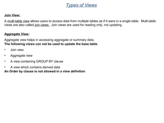
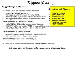
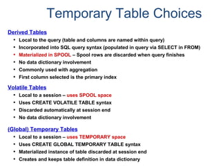
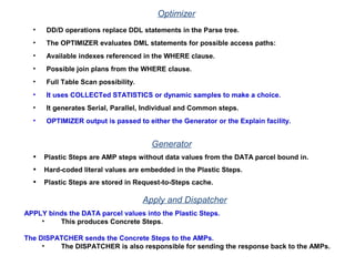
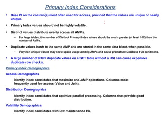
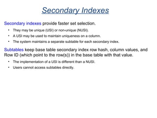
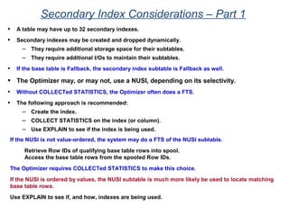
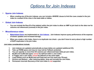
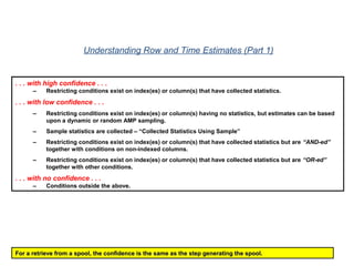
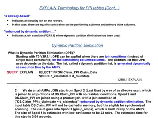
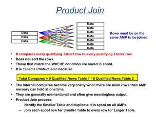
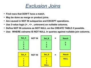
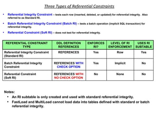
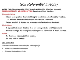
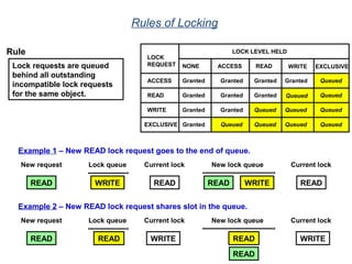
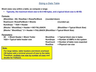
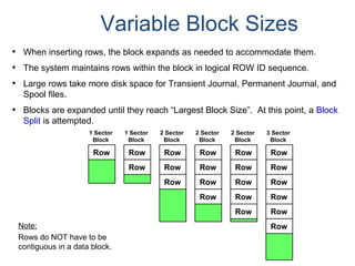
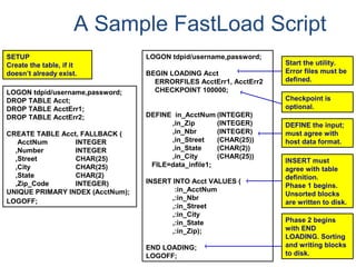
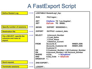
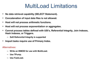
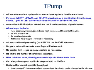
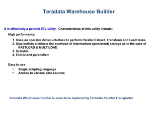
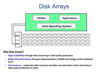
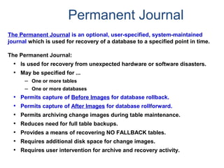
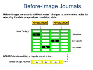
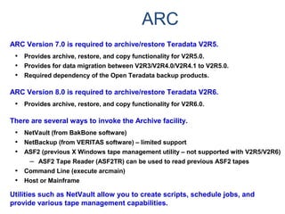
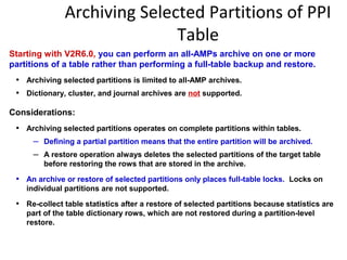
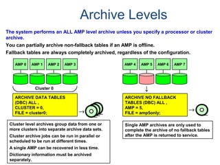
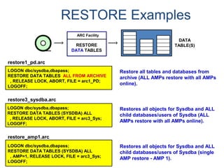
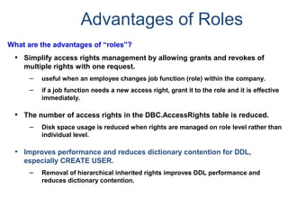
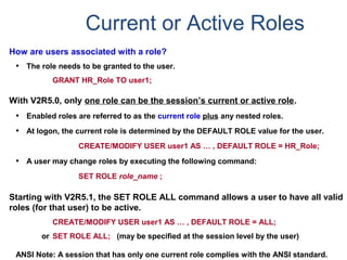
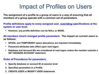
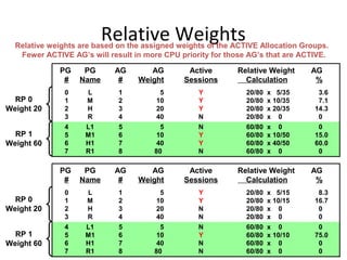
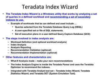
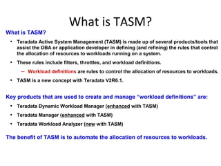
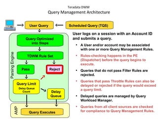
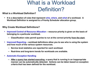
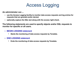
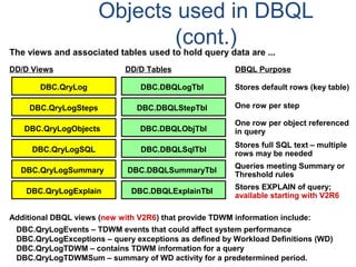
![COLLECT STATISTICS on a Data Sample
SAMPLING reduces resource usage by collecting on a percentage of the data.
• System determines appropriate sample size to generate accurate statistics.
• Syntax option is: COLLECT STATISTICS [USING SAMPLE] ...]
• Re-collection collects statistics using the same mode (full scan or sampled) as
specified in the initial collection.
– System does not store both sampled and complete statistics for the same index
or column set.
– Only one set of statistics is stored for a given index or column.
• Sampled statistics are more accurate for data that is uniformly distributed.
– Sampling is useful for very large tables with reasonable distribution of data.
– Sampling should not be considered for highly skewed data as the Optimizer
needs to be aware of such skew.
– Sampling is more appropriate for indexes than non-indexed column(s).](https://image.slidesharecdn.com/teradataa-z-160821064323/85/Teradata-a-z-70-320.jpg)
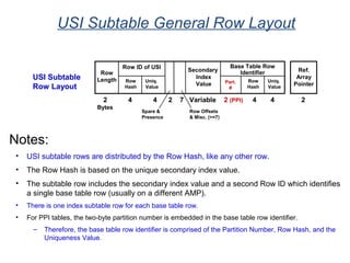
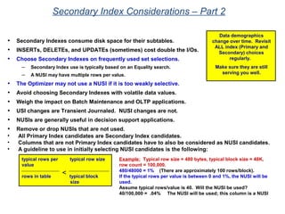
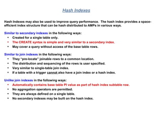
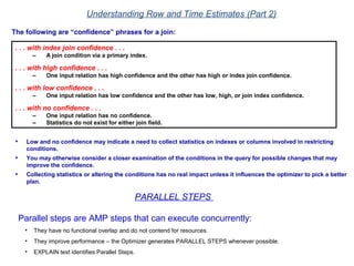
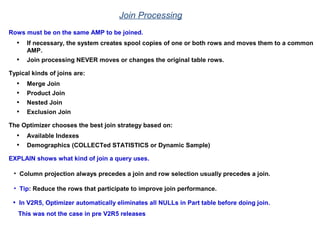
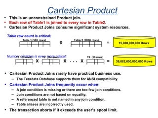
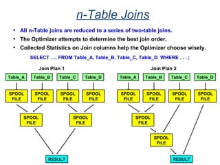
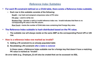
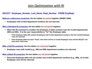
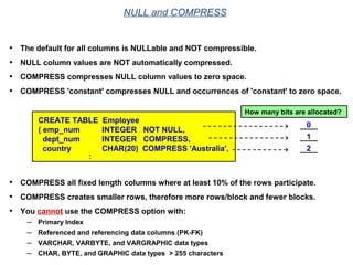
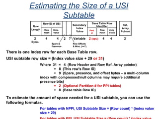
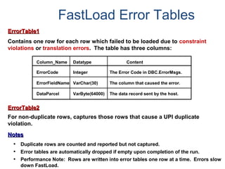
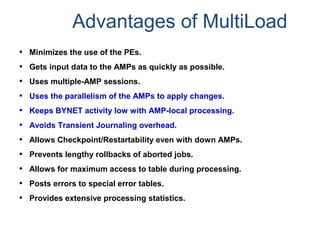
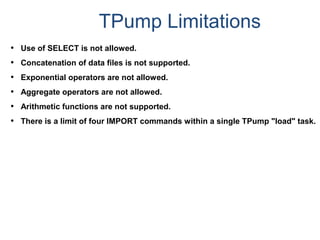

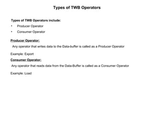
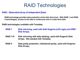
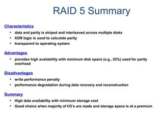
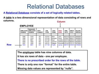
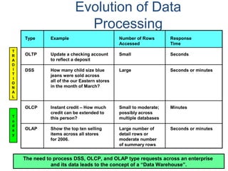
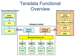
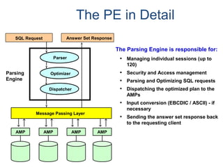
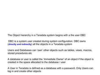
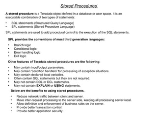
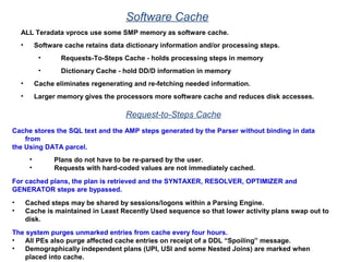
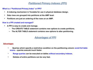
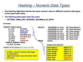
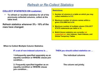
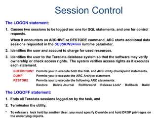
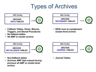
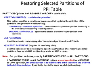
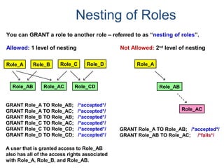
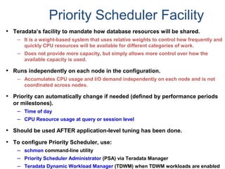
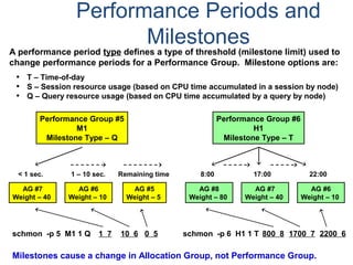
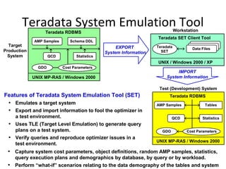
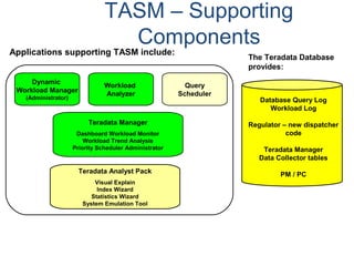
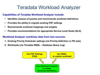
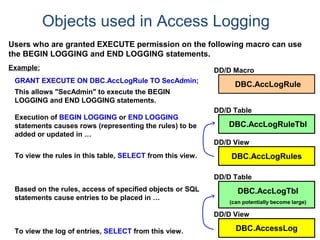
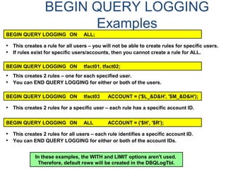
![Assigning Tables to a
Permanent JournalDATABASE
Single
Table
Permanent
Journal
#1
DATABASE
Multiple
Tables
Permanent
Journal
#2
DATABASE
Multiple
Tables
DATABASE
Permanent
Journal
DATABASE
Multiple
Tables
DATABASE
Table_A
Table_B
Table_C
Table_D
Permanent
Journal
#3
#4
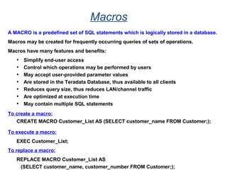
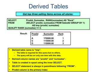
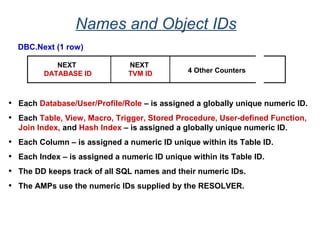
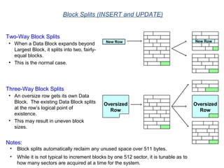
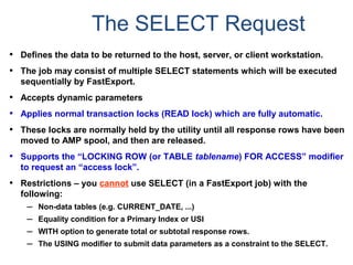
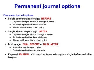
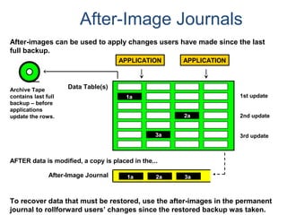
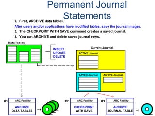
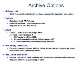
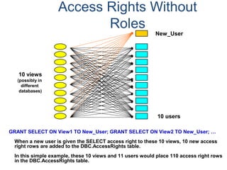
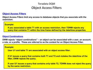
No database or user may contain more than
one permanent journal table.
The journal table may be located:
• In the same database [ #1, #2 and #4 ]
or
• In a different database than the data tables
[#3 & #4]](https://image.slidesharecdn.com/teradataa-z-160821064323/85/Teradata-a-z-177-320.jpg)
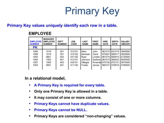
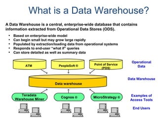
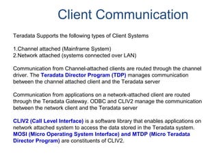
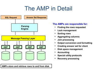
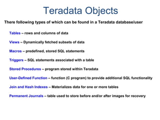
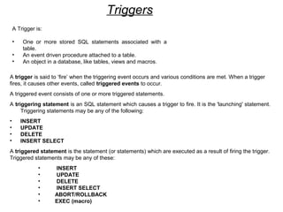
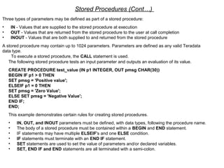
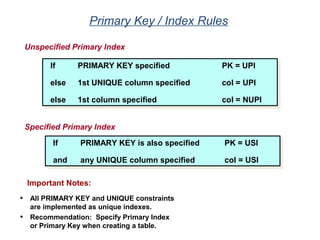
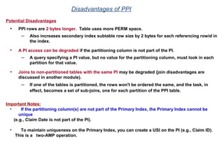
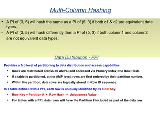
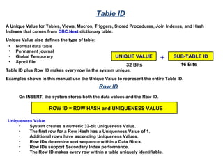
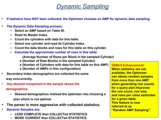
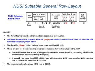
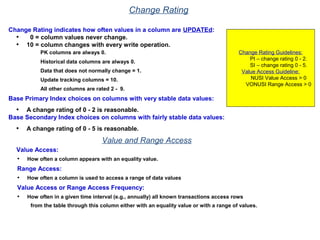
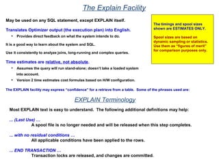
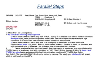
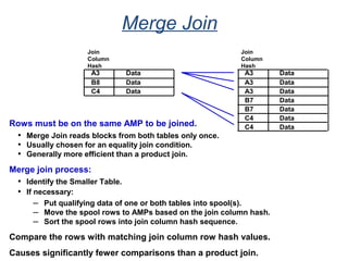
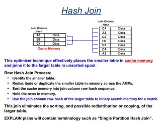
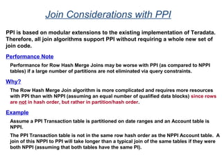
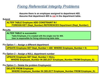
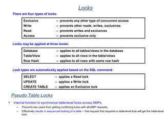
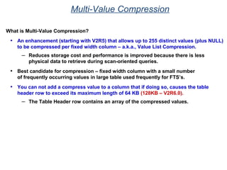
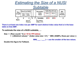
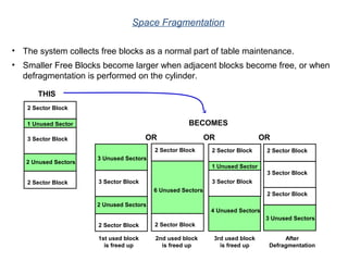
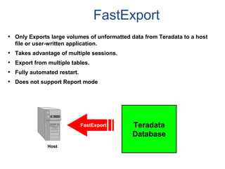
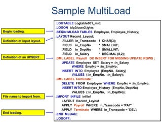
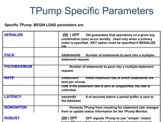
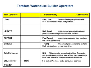
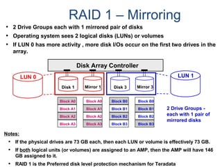
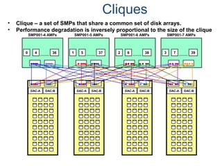
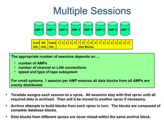
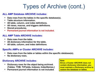
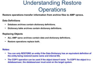
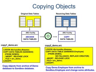
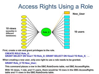
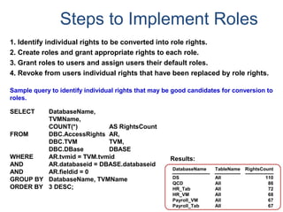
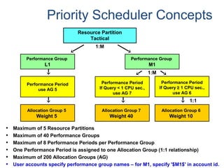
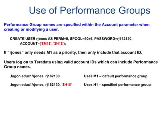
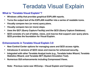
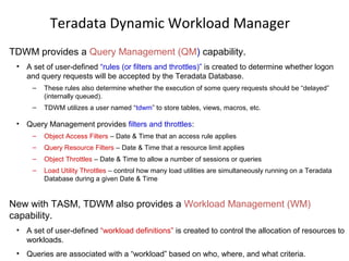
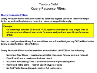
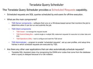
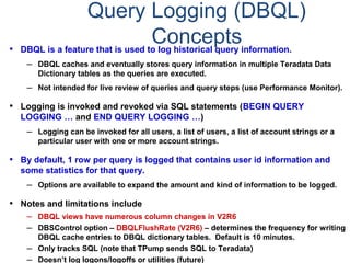
![Assigning a Permanent
Journal
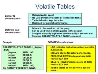
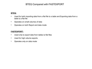
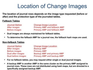
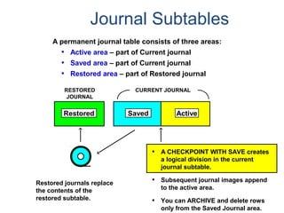
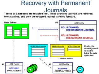
{ CREATE USER | CREATE DATABASE } . . .
[ [ [ NO | DUAL ] [ AFTER | BEFORE ] JOURNAL ] . . . ]
[ DEFAULT JOURNAL TABLE = journal_name ] ;
Default journal values at the database levels are:
Journal Option Default
NONE SPECIFIED NO JOURNAL MAINTAINED
NEITHER AFTER NOR BEFORE BOTH TYPES IMPLIED
NEITHER DUAL NOR NO FALLBACK – DUAL IMAGES; NO FALLBACK – SINGLE IMAGES
At the table level, you can indicate journal options with the CREATE statement:
CREATE TABLE . . .
[ [ [ NO | DUAL ] [ AFTER | BEFORE ] JOURNAL ] ... ]
[ WITH JOURNAL TABLE = journal_name ] ;
Default journal values at the table levels are :
Journal Option Default
NONE SPECIFIED Defaults to USER/DATABASE
AFTER IMAGE ONLY Defaults FOR BEFORE IMAGE
BEFORE IMAGE ONLY Defaults FOR AFTER IMAGE
NEITHER DUAL NOR NO Defaults to PROTECTION TYPE
Note: If a database or
user that contains a
permanent journal runs
out of space, all table
updates that write to that
journal abort.](https://image.slidesharecdn.com/teradataa-z-160821064323/85/Teradata-a-z-179-320.jpg)
![Profiles
What is a “profile”?
• A profile is a set of common user parameters that can be applied to a group
of users.
• Profile parameters include:
– Account id(s)
– Default database
– Spool space allocation
– Temporary space allocation
– Password attributes (expiration, etc.)
What is the advantages of using “profiles”?
• Profiles simplify user management.
– A change of a common parameter requires an update of a profile instead of each
individual user affected by the change.
How are “profiles” managed?
• New DDL commands, tables, view, command options, and access rights.
– CREATE PROFILE, MODIFY PROFILE, DROP PROFILE, and SELECT PROFILE
– New system table - DBC.Profiles
– New system views - DBC.ProfileInfo[x]](https://image.slidesharecdn.com/teradataa-z-160821064323/85/Teradata-a-z-211-320.jpg)
![Data Dictionary Views
DBC.Children[X] Hierarchical relationship information. * – X view is new
with V2R6
DBC.Databases[X] Database, user and immediate parent information.
DBC.Users Similar to Databases view, but includes columns specific to
users.
DBC.Tables[X] Tables, views, macros, triggers, and stored procedures
information.
DBC.ShowTblChecks[X] * Database table constraint information.
DBC.ShowColChecks[X] * Database column constraint information.
DBC.Columns[X] Information about columns/parameters in tables, views, and
macros.
DBC.Indices[X] Table index information.
DBC.IndexConstraints[X] * Provides information about index constraints, e.g., PPI
definition.](https://image.slidesharecdn.com/teradataa-z-160821064323/85/Teradata-a-z-243-320.jpg)

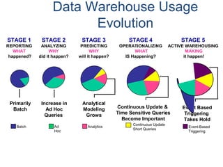
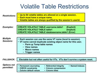
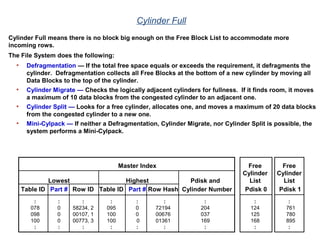
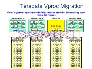
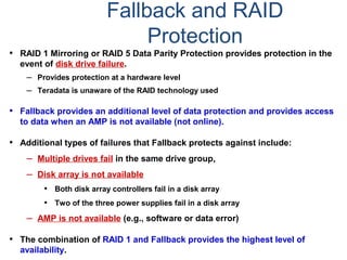
The document provides an overview of database fundamentals including what a database is, relational databases, primary keys, foreign keys, advantages of relational databases, data warehousing, active data warehousing, and Teradata. Key points include: - A database is a collection of logically related and shared data that is protected and managed. - A relational database consists of related tables with rows and columns. Primary keys uniquely identify rows and foreign keys define relationships between tables. - Relational databases are easy to use, understand, and allow for flexible responses to changing business needs. - A data warehouse contains extracted and consolidated data from operational systems for analysis and reporting. - Active data warehousing provides timely access


![[Www.pkbulk.blogspot.com]dbms01](https://cdn.slidesharecdn.com/ss_thumbnails/www-pkbul-blogspot-comdbms01-130615034553-phpapp01-thumbnail.jpg?width=640&height=640&fit=bounds)