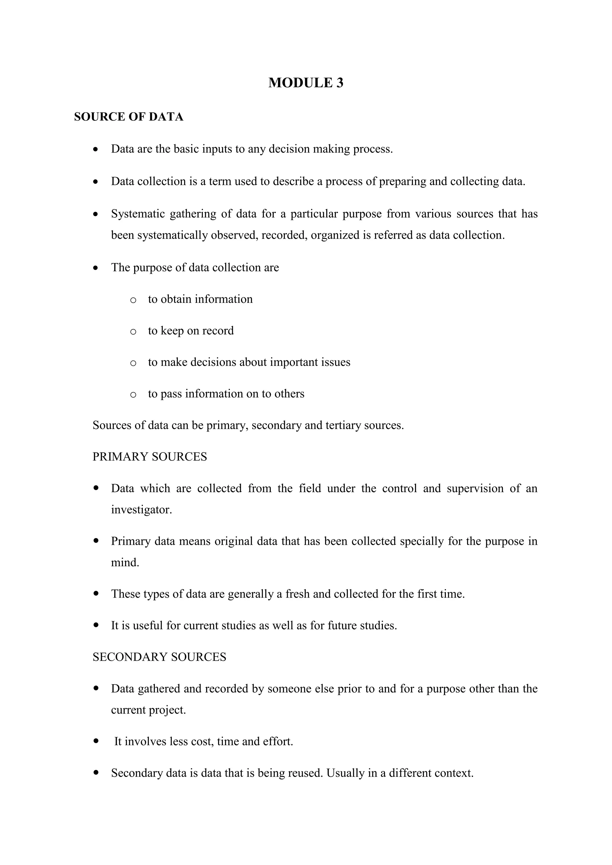
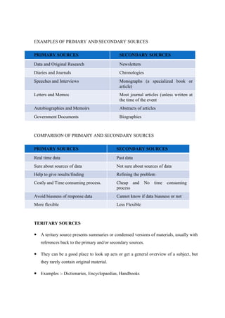
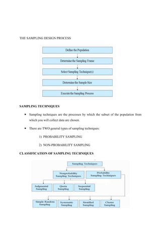
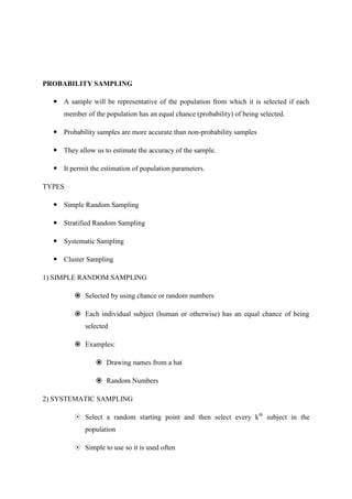
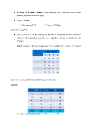
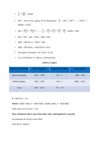
MODULE 3
SOURCE OF DATA
 Data are the basic inputs to any decision making process.
 Data collection is a term used to describe a process of preparing and collecting data.
 Systematic gathering of data for a particular purpose from various sources that has
been systematically observed, recorded, organized is referred as data collection.
 The purpose of data collection are
o to obtain information
o to keep on record
o to make decisions about important issues
o to pass information on to others
Sources of data can be primary, secondary and tertiary sources.
PRIMARY SOURCES
 Data which are collected from the field under the control and supervision of an
investigator.
 Primary data means original data that has been collected specially for the purpose in
mind.
 These types of data are generally a fresh and collected for the first time.
 It is useful for current studies as well as for future studies.
SECONDARY SOURCES
 Data gathered and recorded by someone else prior to and for a purpose other than the
current project.
 It involves less cost, time and effort.
 Secondary data is data that is being reused. Usually in a different context.
EXAMPLES OF PRIMARY AND SECONDARY SOURCES
PRIMARY SOURCES SECONDARY SOURCES
Data and Original Research Newsletters
Diaries and Journals Chronologies
Speeches and Interviews Monographs (a specialized book or
article)
Letters and Memos Most journal articles (unless written at
the time of the event
Autobiographies and Memoirs Abstracts of articles
Government Documents Biographies
COMPARISON OF PRIMARY AND SECONDARY SOURCES
PRIMARY SOURCES SECONDARY SOURCES
Real time data Past data
Sure about sources of data Not sure about sources of data
Help to give results/finding Refining the problem
Costly and Time consuming process. Cheap and No time consuming
process
Avoid biasness of response data Cannot know if data biasness or not
More flexible Less Flexible
TERITARY SOURCES
 A teritary source presents summaries or condensed versions of materials, usually with
references back to the primary and/or secondary sources.
 They can be a good place to look up acts or get a general overview of a subject, but
they rarely contain original material.
 Examples :- Dictionaries, Encyclopaedias, Handbooks
TYPES OF DATA
 Categorical Data
 Nominal Data
 Ordinal Data
CATEGORICAL DATA
 A set of data is said to be categorical if the values or observations belonging to it can
be stored according to category.
 Each value is chosen from a set of non-overlapping categories.
 Eg:-
NOMINAL DATA
 A set of data is said to be nominal if the values or observations belonging to it can be
a code in the form of a number where the numbers are simply labels.
 It is possible to count but not order or measure nominal data.
 Eg :- in a data set males can be coded as 0 and female as 1; marital status of an
individual could be coded as Y if married and N if single.
ORDINAL DATA
 A set of data is said to be ordinal if the values or observations belonging to it can be
ranked or have a rating scale attached.
 Ordinal scales (data) ranks objects from one largest to smallest or first to last and so
on.
 It is possible to count and order but not measure ordinal data.
METHODS OF COLLECTING DATA
 Data are the raw numbers or facts which must be processed to give useful
information.
 Data collection is expensive, so it is sensible to decide what the data will be used for
before they are collected.
 In principle, there is an optimal amount of data which should be collected. These data
should be as accurate as possible.
1. OBSERVATION METHOD
 Observation method is a technique in which the behavior of research subjects is
watched and recorded without any direct contact.
CHARACTERISTICS
 It is the main method of Psychology and serves as the basis of any scientific enquiry.
 Primary material of any study can be collected by this method.
 Observational method of research concerns the planned watching, recording and
analysis of observed method.
 This method requires careful preparation and proper training for the observer.
TYPES OF OBSERVATION
STRUCTURED OBSERVATION UNSTRUCTURED OBSERVATION
• In structured observation, the
researcher specifies in detail what
is to be observed and how the
measurements are to be recorded.
• It is appropriate when the problem
is clearly defined and the
• In unstructured observation, the
researcher monitors all aspects of
the phenomenon that seem relevant.
• It is appropriate when the problem
has yet to be formulated precisely
and flexibility is needed in
information needed is specified. observation to identify key
components of the problem and to
develop hypotheses.
PARTICIPANT OBSERVATION NON PARTICIPANT OBSERVATION
• If the observer observes by making
himself, more or less, a member of
the group he is observing so that he
can experience what the members
of the group experience, then the
observation is called participant
observation.
• When the observer observes as a
detached emissary without any
attempt on his part to experience
through participation what others
feel, the observation of this type is
known as non-participant
observation.
CONTROLLED OBSERVATION UNCONTROLLED OBSERVATION
 If the observation takes place
according to definite pre-arranged
plans, involving experimental
procedure, the same is termed as
controlled observation
• If the observation takes place in the
natural setting, it may be termed as
uncontrolled observation.
OBSERVATION
ADVANTAGES DISADVANTAGES
 Most direct measure of behavior
 Provides direct information
 Easy to complete, saves time
 Can be used in natural or
experimental settings
• May require training
• Observer’s presence may create
artificial situation
• Potential to overlook meaningful
aspects
• Potential for misinterpretation
• Difficult to analyze
FIELD INVESTIGATION
 Any activity aimed at collecting primary (original or otherwise
unavailable) data, using methods such as face-to-face interviewing, surveys and case
study method is termed as field investigation.
 SURVEY
 The survey is a non-experimental, descriptive research method.
 Surveys can be useful when a researcher wants to collect data on phenomena
that cannot be directly observed (such as opinions on library services).
 In a survey, researchers sample a population.
 The Survey method is the technique of gathering data by asking questions to
people who are thought to have desired information.
 A formal list of questionnaire is prepared. Generally a non disguised approach
is used.
 The respondents are asked questions on their demographic interest opinion.
 CASE STUDY METHOD
 Case study method is a common technique used in research to test theoretical
propositions or questions in relation to qualitative inquiry.
 The strength of the case study approach is that it facilitates simultaneous
analysis and comparison of individual cases for the purpose of identifying
particular phenomena among those cases, and for the purpose of more general
theory testing, development or construction.
 A case study is a form of research defined by an interest in individual cases. It
is not a methodology per se, but rather a useful technique or strategy for
conducting qualitative research.
 The more the object of study is a specific, unique, bounded system, the more
likely that it can be characterized as a case study.
 Once the case is chosen, it can be investigated by whatever method is deemed
appropriate to the aims of the study.
 Case studies are particularly useful for examining a phenomena in context.
 The case study methodology is designed to study a phenomenon or set of
interacting phenomena in context ―when the boundaries between phenomenon
and context are not clearly evident.‖
 The lack of distinction between phenomenon and context make case studies
ideal for conducting exploratory research designed to stand alone or to guide
the formulation of further quantitative research.
 Some case studies may be a ‘snap shot’ analysis of a particular event or
occurrence.
 Other case studies may involve consideration of a sequence of events, often
over an extended period of time, in order to better determine the causes of
particular phenomena.
 INTERVIEWS
 Interview is the verbal conversation between two people with the objective of
collecting relevant information for the purpose of research.
 It is possible to use the interview technique as one of the data collection
methods for the research.
 It makes the researcher to feel that the data what he collected is true and
honest and original by nature because of the face to face interaction.
DIRECT STUDIES
 On the basis of reports, records and experimental observations.
SAMPLING
THE SAMPLING DESIGN PROCESS
SAMPLING TECHNIQUES
 Sampling techniques are the processes by which the subset of the population from
which you will collect data are chosen.
 There are TWO general types of sampling techniques:
1) PROBABILITY SAMPLING
2) NON-PROBABILITY SAMPLING
CLASSIFICATION OF SAMPLING TECHNIQUES
PROBABILITY SAMPLING
 A sample will be representative of the population from which it is selected if each
member of the population has an equal chance (probability) of being selected.
 Probability samples are more accurate than non-probability samples
 They allow us to estimate the accuracy of the sample.
 It permit the estimation of population parameters.
TYPES
 Simple Random Sampling
 Stratified Random Sampling
 Systematic Sampling
 Cluster Sampling
1) SIMPLE RANDOM SAMPLING
 Selected by using chance or random numbers
 Each individual subject (human or otherwise) has an equal chance of being
selected
 Examples:
 Drawing names from a hat
 Random Numbers
2) SYSTEMATIC SAMPLING
 Select a random starting point and then select every kth
subject in the
population
 Simple to use so it is used often
3) STRATIFIED SAMPLING
 Divide the population into at least two different groups with common
characteristic(s), then draw SOME subjects from each group (group is called
strata or stratum)
 Results in a more representative sample
4) CLUSTER SAMPLING
 Divide the population into groups (called clusters), randomly select some of
the groups, and then collect data from ALL members of the selected groups
 Used extensively by government and private research organizations
 Examples:
 Exit Polls
NON-PROBABILITY SAMPLING
DEFINITION
The process of selecting a sample from a population without using (statistical) probability
theory.
NOTE THAT IN NON-PROBABILITY SAMPLING
 each element/member of the population DOES NOT have an equal chance of being
included in the sample, and
 the researcher CANNOT estimate the error caused by not collecting data from all
elements/members of the population.
TYPES
 Quota Sampling
 Judgemental Sampling
 Sequential Sampling
1) QUOTA SAMPLING
 Selecting participant in numbers proportionate to their numbers in the larger
population, no randomization.
 For example you include exactly 50 males and 50 females in a sample of 100.
2) JUDGMENTAL SAMPLING
 It is a form of sampling in which population elements are selected based on the
judgment of the researcher.
3) SEQUENTIAL SAMPLING
 Sequential sampling is a non-probability sampling technique wherein the researcher
picks a single or a group of subjects in a given time interval, conducts his study,
analyzes the results then picks another group of subjects if needed and so on.
DATA PROCESSING AND ANALYSIS STRATEGIES
 EDITING
o The process of checking and adjusting responses in the completed
questionnaires for omissions, legibility, and consistency and readying them for
coding and storage.
o Types
 Field Editing
 Preliminary editing by a field supervisor on the same day as the
interview to catch technical omissions, check legibility of
handwriting, and clarify responses that are logically or
conceptually inconsistent.
 In-house Editing
 Editing performed by a central office staff; often dome more
rigorously than field editing
 DATA CODING
o A systematic way in which to condense extensive data sets into smaller
analyzable units through the creation of categories and concepts derived from
the data.
o The process by which verbal data are converted into variables and categories
of variables using numbers, so that the data can be entered into computers for
analysis.
 CLASSIFICATION
o Most research studies result in a large volume of raw data which must be
reduced into homogeneous groups if we are to get meaningful relationships.
o Classification can be one of the following two types, according to the nature of
the phenomenon involved.
 Classification according to attributes : Data are classified on the basis
of common characteristics which can be either descriptive or
numerical.
 Classification according to class interval : Data are classified on the
basis of statistics of variables.
 TABULATION
 When a mass of data has been assembled, it becomes necessary for the
researcher to arrange the same in some kind of concise and logical order. This
procedure is referred to as tabulation.
 Tabulation is an orderly arrangement of data in rows and columns.
 Tabulation is essential because :
 It conserves space and reduces explanatory and descriptive statement
to a minimum.
 It facilitates the process of comparison.
 It provides a basis for various statistical computation.
 It facilitates the summation of items and detection of errors and
omissions.
GRAPHICAL REPRESENTATION
Graphs are pictorial representations of the relationships between two (or more)
variables and are an important part of descriptive statistics. Different types of graphs can be
used for illustration purposes depending on the type of variable (nominal, ordinal, or interval)
and the issues of interest. The various types of graphs are :
Line Graph: Line graphs use a single line to connect plotted points of interval and, at times,
nominal data. Since they are most commonly used to visually represent trends over time, they
are sometimes referred to as time-series charts.
Advantages - Line graphs can:
 clarify patterns and trends over time better than most other graphs be visually simpler
than bar graphs or histograms
 summarize a large data set in visual form
 become more smooth as data points and categories are added
 be easily understood due to widespread use in business and the media
 require minimal additional written or verbal explanation
Disadvantages - Line graphs can:
 be inadequate to describe the attribute, behavior, or condition of interest
 fail to reveal key assumptions, norms, or causes in the data
 be easily manipulated to yield false impressions
 reveal little about key descriptive statistics, skew, or kurtosis
 fail to provide a check of the accuracy or reasonableness of calculations
Bar graphs are commonly used to show the number or proportion of nominal or ordinal data
which possess a particular attribute. They depict the frequency of each category of data points
as a bar rising vertically from the horizontal axis. Bar graphs most often represent the number
of observations in a given category, such as the number of people in a sample falling into a
given income or ethnic group. They can be used to show the proportion of such data points,
but the pie chart is more commonly used for this purpose. Bar graphs are especially good for
showing how nominal data change over time.
Advantages – Bar graphs can:
 show each nominal or ordinal category in a frequency distribution
 display relative numbers or proportions of multiple categories
 summarize a large data set in visual form
 clarify trends better than do tables or arrays
 estimate key values at a glance
 permit a visual check of the accuracy and reasonableness of calculations
 be easily understood due to widespread use in business and the media
Disadvantages – Bar graphs can:
 require additional written or verbal explanation
 be easily manipulated to yield false impressions
 be inadequate to describe the attribute, behavior, or condition of interest
 fail to reveal key assumptions, norms, causes, effects, or patterns
Histograms are the preferred method for graphing grouped interval data. They depict the
number or proportion of data points falling into a given class. For example, a histogram
would be appropriate for depicting the number of people in a sample aged 18-35, 36-60, and
over 65. While both bar graphs and histograms use bars rising vertically from the horizontal
axis, histograms depict continuous classes of data rather than the discrete categories found in
bar charts. Thus, there should be no space between the bars of a histogram.
Advantages - Histograms can:
 begin to show the central tendency and dispersion of a data set
 closely resemble the bell curve if sufficient data and classes are used
 show each interval in the frequency distribution
 summarize a large data set in visual form
 clarify trends better than do tables or arrays
 estimate key values at a glance permit a visual check of the accuracy and
reasonableness of calculations
 be easily understood due to widespread
 use in business and the media use bars whose areas reflect the proportion of data
points in each class
Disadvantages - Histograms can:
 require additional written or verbal explanation
 be easily manipulated to yield false impressions
 be inadequate to describe the attribute, behavior, or condition of interest
 fail to reveal key assumptions, norms, causes, effects, or pattern
DESCRIPTIVE AND INFERENTIAL DATA ANALYSIS
 Descriptive analysis is the study of distributions of one variable (described as
unidimensional analysis) or two variables (described as bivariate analysis) or more
than two variables (described as multivariate analysis).
 Is devoted to summarization and description of data.
 Inferential analysis is mainly on the basis of various test of significance for testing
hypothesis inorder to determine with what validity data can be said to indicate some
conclusions.
 Uses sample data to make inferences about a population
CORRELATION ANALYSIS
 Correlation a LINEAR association between two random variables.
 Correlation analysis shows us how to determine both the nature and strength of
relationship between two variables.
 When variables are dependent on time correlation is applied.
 Correlation lies between +1 to -1.
 A zero correlation indicates that there is no relationship between the variables.
 A correlation of –1 indicates a perfect negative correlation.
 A correlation of +1 indicates a perfect positive correlation.
SPEARMAN’S RANK COEFFICIENT
 A method to determine correlation when the data is not available in numerical form
and as an alternative method, the method of rank correlation is used.
 Thus when the values of the two variables are converted to their ranks, and there from
the correlation is obtained, the correlations known as rank correlation.
Spearman’s rank correlation coefficient ρ can be calculated when:
 Actual ranks given
 Ranks are not given but grades are given but not repeated
 Ranks are not given and grades are given and repeated
Where, di = difference between ranks of ith pair of two variables
n = no. of pairs of observations
KARL PEARSON’S COEFFICIENT OF CORRELATION
 Correlation is a useful technique for investigating the relationship between two
quantitative, continuous variables. Pearson's correlation coefficient ( ) is a measure
of the strength of the association between the two variables.
 Karl Pearson’s coefficient of correlation, =
∑ ̅̅̅ ̅̅̅
 ---- Standard deviation of random variable x,y
 ̅, ̅ ------ average/arithmetic mean
LEAST SQUARE METHOD
 The method of least squares is a standard approach to the approximate solution of
over determined systems, i.e., sets of equations in which there are more equations
than unknowns.
 "Least squares" means that the overall solution minimizes the sum of the squares of
the errors made in the results of every single equation.
 The goal is to find the parameter values for the model which ―best‖ fits the data.
PROBLEM STATEMENT
 The objective consists of adjusting the parameters of a model function to best fit a
data set.
 A simple data set consists of n points (data pairs) , i = 1, ..., n, where is an
independent variable and is a dependent variable whose value is found by
observation.
 The model function has the form f(x,β), where the m adjustable parameters are held in
the vector β.
 The least squares method finds its optimum when the sum, S, of squared residuals
∑ ,
where
is a minimum.
 A residual is defined as the difference between the actual value of the dependent
variable and the value predicted by the model.
DATA ANALYSIS USING STATISTICAL PACKAGES
I) CHI-SQUARE TEST
 The chi-square test is an important test amongst the several tests of significance
developed by statisticians.
 It was developed by Karl Pearson in1900.
 CHI SQUARE TEST is a non parametric test not based on any assumption or
distribution of any variable.
 This statistical test follows a specific distribution known as chi square distribution.
 In general, the test we use to measure the differences between what is observed and
what is expected according to an assumed hypothesis is called the chi-square test.
STEPS FOR CHI SQUARE TEST
1) Set up the null hypothesis that there is goodness of fit between observed and expected
frequencies.
2) Find the value of using the formula ∑
where O : observed frequencies ,
E : expected frequencies
3) Degree of freedom is n-1 where n is the no. of frequencies given.
4) Obtain the table value.
5) If the calculated is less than table value, conclude that there is goodness of fit.
The goodness of fit indicates that the difference if any is only due to fluctuations in sampling.
EXAMPLE
HO: Horned lizards eat equal amounts of leaf cutter, carpenter and black ants.
HA: Horned lizards eat more amounts of one species of ants than the others.
Leaf Cutter
Ants
Carpenter
Ants
Black Ants Total
Observed 25 18 17 60
Expected 20 20 20 60
O-E 5 -2 -3 0
(O-E)2
E
1.25 0.2 0.45 χ2
= 1.90
∑
Calculate degrees of freedom: (n-1)= 3-1 = 2
Under a critical value of your choice (e.g. α = 0.05 or 95% confidence), look up Chi-square
statistic on a Chi-square distribution table.
Chi-square statistic: χ2
= 5.991 Our calculated value: χ2
= 1.90
*If chi-square statistic > your calculated value, conclude that there is goodness of fit.
5.991 > 1.90 ∴ we accept the hypothesis that there is goodness of fit between observed and
expected values..
II) ANALYSIS OF VARIANCE (ANOVA)
 ANalysis Of VAriance (ANOVA) is the technique used to determine whether more
than two population means are equal.
 Types of ANOVA
1) One way ANOVA 2) Two way ANOVA
ONE WAY ANOVA
 The ANOVA used for the studying the differences among the influence of various
categories of independent variables on a dependent variable is called one way
ANOVA.
Q) Below are given the yield (in kg per acre for 5 trial plots of 4 varieties of treatment
PLOT
NO.
TREATMENT
1 2 3 4
1 42 48 68 80
2 50 66 52 94
3 62 68 76 78
4 34 78 64 82
5 52 70 70 66
Carry out an analysis of variance and state your conclusions.
Solution
I (x1) II (x2) III (x3) IV (x4)
42 48 68 80
50 66 52 94
62 68 76 78
34 78 64 82
52 70 70 66
240 330 330 400
• T = Sum of all the observations = 42+50+….+66 = 1300
• = = 84500
• SST = Sum of the squares of all observations - = (
• SSC =
∑
+
∑
+ ….. - = + + - 84500 = 2580
• SSE = SST – SSC = 4236 – 2580 =1656
• MSC = SSC/(k-1) = 2580/3 = 860
• MSE = SSE/(N-k) = 1656/(20-4) =103.5
• The degree of freedom = (k-1,N-k) = (3,16)
• k: no. of columns; N : total no. of observations
ANOVA TABLE
Sources of Variation Sum of Squares Degree of freedom Mean Square
Between Samples SSC = 2580 K-1 = 3 MSC = 860
Within Samples SSE = 1656 N-k = 1 MSE = 103.5
Total SST = 4236 N-1 = 19
F = 860/103.5 = 8.3
NOTE: If MSC>MSE, F = MSC/MSE; If MSC<MSE, F = MSE/MSC
Table value of F at (3,16) = 3.24
Since calculated value is more than table value, null hypothesis is rejected.
So treatments do not have same effect
TWO WAY ANOVA
 ANOVA used for studying the difference among the influence of various categories
of two independent variables on a dependent variable is called two way ANOVA.
HYPOTHESIS TESTING
Hypothesis: An assertion (assumption) about some characteristic of the population(s), which
should be supported or rejected on the basis of empirical evidence obtained from the
sample(s).
Research Hypothesis: An assumption about the outcome of research (solution to the
problem facing the society or answer to the question).
Statistical Hypothesis: An assumption about any characteristic of the population(s),
expressed in statistical terms (parameter such as population mean, population variance,
population proportion, form of the population distribution etc.).
PARAMETRIC AND NON PARAMETRIC TEST
PARAMETRIC TEST
• If the information about the population is completely known by means of its
parameters then statistical test is called parametric test
• ∗ Eg: t- test, f-test, z-test, ANOVA test
NON- PARAMETRIC TEST
• If there is no knowledge about the population or parameters, but still it is required to
test the hypothesis of the population. Then it is called non-parametric test
• ∗ Eg: Chi-square test, Mann-Whitney, rank sum test, Kruskal-Wallis test
NULL HYPOTHESIS vs. ALTERNATIVE HYPOTHESIS
Null Hypothesis
• Statement about the value of a population parameter
• Represented by H0
• Always stated as an Equality
Alternative Hypothesis
• Statement about the value of a population parameter that must be true if the null
hypothesis is false
• Represented by H1
• Stated in on of three forms
• >, <, 
• Example: Consider a set of children having complan and another set having horlicks:
if both have same result for the children then this is consider as null hypothesis and
have difference is alternate hypothesis. After data analysis, if there is a difference in
result then null hypothesis is rejected so there is a scope for the further research.
There can be errors while testing a hypothesis. These errors can be classified into two:
TYPE I vs TYPE II ERROR
Type I error – Rejecting Ho when Ho is true
Type II error – Accepting Ho when Ho is false
LEVEL OF SIGNIFICANCE
• In hypothesis testing, the null hypothesis is either accepted or rejected, depending on
whether the p value is above or below a predetermined cut-off point, known as the
Significance level of the test, usually it is taken as 5% level.
P value
• P is the probability of being wrong when H0 rejected.
• When the level of Significance is set at 5% and the test statistics fall in the region of
rejection, then the p value must be less than 5% i.e (p<0.05).
• When we will accept H0 (p>0.05).
ALPHA vs. BETA
 α is the probability of Type I error
 β is the probability of Type II error
 The experimenters (you and I) have the freedom to set the -level for a particular
hypothesis test. That level is called the level of significance for the test. Changing α
can (and often does) affect the results of the test—whether you reject or fail to reject
H0.
ONE TAILED TEST
 In left tailed test, calculated value is less than table value, we reject Ho
 In right tailed test, calculated value is greater than table value, we reject Ho
TWO TAILED TEST
 If calculated value lies in the acceptance region, then we accept null hypothesis
 If calculated value is outside acceptance region, we reject null hypothesis
STEPS FOR HYPOTHESIS TESTING
INTERPRETATION
• Interpretation refers to the task of drawing inferences from the collected facts after an
analytical and/or experimental study.
• Task of interpretation:
• The effort to establish continuity in research through linking the results of a
given study with those of another
• The establishment of some explanatory concepts
Data Collection And Analysis

Data Collection And Analysis

  • 1.
    MODULE 3 SOURCE OFDATA  Data are the basic inputs to any decision making process.  Data collection is a term used to describe a process of preparing and collecting data.  Systematic gathering of data for a particular purpose from various sources that has been systematically observed, recorded, organized is referred as data collection.  The purpose of data collection are o to obtain information o to keep on record o to make decisions about important issues o to pass information on to others Sources of data can be primary, secondary and tertiary sources. PRIMARY SOURCES  Data which are collected from the field under the control and supervision of an investigator.  Primary data means original data that has been collected specially for the purpose in mind.  These types of data are generally a fresh and collected for the first time.  It is useful for current studies as well as for future studies. SECONDARY SOURCES  Data gathered and recorded by someone else prior to and for a purpose other than the current project.  It involves less cost, time and effort.  Secondary data is data that is being reused. Usually in a different context.
  • 2.
    EXAMPLES OF PRIMARYAND SECONDARY SOURCES PRIMARY SOURCES SECONDARY SOURCES Data and Original Research Newsletters Diaries and Journals Chronologies Speeches and Interviews Monographs (a specialized book or article) Letters and Memos Most journal articles (unless written at the time of the event Autobiographies and Memoirs Abstracts of articles Government Documents Biographies COMPARISON OF PRIMARY AND SECONDARY SOURCES PRIMARY SOURCES SECONDARY SOURCES Real time data Past data Sure about sources of data Not sure about sources of data Help to give results/finding Refining the problem Costly and Time consuming process. Cheap and No time consuming process Avoid biasness of response data Cannot know if data biasness or not More flexible Less Flexible TERITARY SOURCES  A teritary source presents summaries or condensed versions of materials, usually with references back to the primary and/or secondary sources.  They can be a good place to look up acts or get a general overview of a subject, but they rarely contain original material.  Examples :- Dictionaries, Encyclopaedias, Handbooks
  • 3.
    TYPES OF DATA Categorical Data  Nominal Data  Ordinal Data CATEGORICAL DATA  A set of data is said to be categorical if the values or observations belonging to it can be stored according to category.  Each value is chosen from a set of non-overlapping categories.  Eg:- NOMINAL DATA  A set of data is said to be nominal if the values or observations belonging to it can be a code in the form of a number where the numbers are simply labels.  It is possible to count but not order or measure nominal data.  Eg :- in a data set males can be coded as 0 and female as 1; marital status of an individual could be coded as Y if married and N if single. ORDINAL DATA  A set of data is said to be ordinal if the values or observations belonging to it can be ranked or have a rating scale attached.  Ordinal scales (data) ranks objects from one largest to smallest or first to last and so on.  It is possible to count and order but not measure ordinal data.
  • 4.
    METHODS OF COLLECTINGDATA  Data are the raw numbers or facts which must be processed to give useful information.  Data collection is expensive, so it is sensible to decide what the data will be used for before they are collected.  In principle, there is an optimal amount of data which should be collected. These data should be as accurate as possible. 1. OBSERVATION METHOD  Observation method is a technique in which the behavior of research subjects is watched and recorded without any direct contact. CHARACTERISTICS  It is the main method of Psychology and serves as the basis of any scientific enquiry.  Primary material of any study can be collected by this method.  Observational method of research concerns the planned watching, recording and analysis of observed method.  This method requires careful preparation and proper training for the observer. TYPES OF OBSERVATION STRUCTURED OBSERVATION UNSTRUCTURED OBSERVATION • In structured observation, the researcher specifies in detail what is to be observed and how the measurements are to be recorded. • It is appropriate when the problem is clearly defined and the • In unstructured observation, the researcher monitors all aspects of the phenomenon that seem relevant. • It is appropriate when the problem has yet to be formulated precisely and flexibility is needed in
  • 5.
    information needed isspecified. observation to identify key components of the problem and to develop hypotheses. PARTICIPANT OBSERVATION NON PARTICIPANT OBSERVATION • If the observer observes by making himself, more or less, a member of the group he is observing so that he can experience what the members of the group experience, then the observation is called participant observation. • When the observer observes as a detached emissary without any attempt on his part to experience through participation what others feel, the observation of this type is known as non-participant observation. CONTROLLED OBSERVATION UNCONTROLLED OBSERVATION  If the observation takes place according to definite pre-arranged plans, involving experimental procedure, the same is termed as controlled observation • If the observation takes place in the natural setting, it may be termed as uncontrolled observation. OBSERVATION ADVANTAGES DISADVANTAGES  Most direct measure of behavior  Provides direct information  Easy to complete, saves time  Can be used in natural or experimental settings • May require training • Observer’s presence may create artificial situation • Potential to overlook meaningful aspects • Potential for misinterpretation • Difficult to analyze
  • 6.
    FIELD INVESTIGATION  Anyactivity aimed at collecting primary (original or otherwise unavailable) data, using methods such as face-to-face interviewing, surveys and case study method is termed as field investigation.  SURVEY  The survey is a non-experimental, descriptive research method.  Surveys can be useful when a researcher wants to collect data on phenomena that cannot be directly observed (such as opinions on library services).  In a survey, researchers sample a population.  The Survey method is the technique of gathering data by asking questions to people who are thought to have desired information.  A formal list of questionnaire is prepared. Generally a non disguised approach is used.  The respondents are asked questions on their demographic interest opinion.  CASE STUDY METHOD  Case study method is a common technique used in research to test theoretical propositions or questions in relation to qualitative inquiry.  The strength of the case study approach is that it facilitates simultaneous analysis and comparison of individual cases for the purpose of identifying particular phenomena among those cases, and for the purpose of more general theory testing, development or construction.  A case study is a form of research defined by an interest in individual cases. It is not a methodology per se, but rather a useful technique or strategy for conducting qualitative research.  The more the object of study is a specific, unique, bounded system, the more likely that it can be characterized as a case study.
  • 7.
     Once thecase is chosen, it can be investigated by whatever method is deemed appropriate to the aims of the study.  Case studies are particularly useful for examining a phenomena in context.  The case study methodology is designed to study a phenomenon or set of interacting phenomena in context ―when the boundaries between phenomenon and context are not clearly evident.‖  The lack of distinction between phenomenon and context make case studies ideal for conducting exploratory research designed to stand alone or to guide the formulation of further quantitative research.  Some case studies may be a ‘snap shot’ analysis of a particular event or occurrence.  Other case studies may involve consideration of a sequence of events, often over an extended period of time, in order to better determine the causes of particular phenomena.  INTERVIEWS  Interview is the verbal conversation between two people with the objective of collecting relevant information for the purpose of research.  It is possible to use the interview technique as one of the data collection methods for the research.  It makes the researcher to feel that the data what he collected is true and honest and original by nature because of the face to face interaction. DIRECT STUDIES  On the basis of reports, records and experimental observations. SAMPLING
  • 8.
    THE SAMPLING DESIGNPROCESS SAMPLING TECHNIQUES  Sampling techniques are the processes by which the subset of the population from which you will collect data are chosen.  There are TWO general types of sampling techniques: 1) PROBABILITY SAMPLING 2) NON-PROBABILITY SAMPLING CLASSIFICATION OF SAMPLING TECHNIQUES
  • 9.
    PROBABILITY SAMPLING  Asample will be representative of the population from which it is selected if each member of the population has an equal chance (probability) of being selected.  Probability samples are more accurate than non-probability samples  They allow us to estimate the accuracy of the sample.  It permit the estimation of population parameters. TYPES  Simple Random Sampling  Stratified Random Sampling  Systematic Sampling  Cluster Sampling 1) SIMPLE RANDOM SAMPLING  Selected by using chance or random numbers  Each individual subject (human or otherwise) has an equal chance of being selected  Examples:  Drawing names from a hat  Random Numbers 2) SYSTEMATIC SAMPLING  Select a random starting point and then select every kth subject in the population  Simple to use so it is used often
  • 10.
    3) STRATIFIED SAMPLING Divide the population into at least two different groups with common characteristic(s), then draw SOME subjects from each group (group is called strata or stratum)  Results in a more representative sample 4) CLUSTER SAMPLING  Divide the population into groups (called clusters), randomly select some of the groups, and then collect data from ALL members of the selected groups  Used extensively by government and private research organizations  Examples:  Exit Polls NON-PROBABILITY SAMPLING DEFINITION The process of selecting a sample from a population without using (statistical) probability theory. NOTE THAT IN NON-PROBABILITY SAMPLING  each element/member of the population DOES NOT have an equal chance of being included in the sample, and  the researcher CANNOT estimate the error caused by not collecting data from all elements/members of the population. TYPES  Quota Sampling  Judgemental Sampling
  • 11.
     Sequential Sampling 1)QUOTA SAMPLING  Selecting participant in numbers proportionate to their numbers in the larger population, no randomization.  For example you include exactly 50 males and 50 females in a sample of 100. 2) JUDGMENTAL SAMPLING  It is a form of sampling in which population elements are selected based on the judgment of the researcher. 3) SEQUENTIAL SAMPLING  Sequential sampling is a non-probability sampling technique wherein the researcher picks a single or a group of subjects in a given time interval, conducts his study, analyzes the results then picks another group of subjects if needed and so on. DATA PROCESSING AND ANALYSIS STRATEGIES  EDITING o The process of checking and adjusting responses in the completed questionnaires for omissions, legibility, and consistency and readying them for coding and storage. o Types  Field Editing
  • 12.
     Preliminary editingby a field supervisor on the same day as the interview to catch technical omissions, check legibility of handwriting, and clarify responses that are logically or conceptually inconsistent.  In-house Editing  Editing performed by a central office staff; often dome more rigorously than field editing  DATA CODING o A systematic way in which to condense extensive data sets into smaller analyzable units through the creation of categories and concepts derived from the data. o The process by which verbal data are converted into variables and categories of variables using numbers, so that the data can be entered into computers for analysis.  CLASSIFICATION o Most research studies result in a large volume of raw data which must be reduced into homogeneous groups if we are to get meaningful relationships. o Classification can be one of the following two types, according to the nature of the phenomenon involved.  Classification according to attributes : Data are classified on the basis of common characteristics which can be either descriptive or numerical.  Classification according to class interval : Data are classified on the basis of statistics of variables.  TABULATION  When a mass of data has been assembled, it becomes necessary for the researcher to arrange the same in some kind of concise and logical order. This procedure is referred to as tabulation.  Tabulation is an orderly arrangement of data in rows and columns.  Tabulation is essential because :  It conserves space and reduces explanatory and descriptive statement to a minimum.  It facilitates the process of comparison.  It provides a basis for various statistical computation.
  • 13.
     It facilitatesthe summation of items and detection of errors and omissions. GRAPHICAL REPRESENTATION Graphs are pictorial representations of the relationships between two (or more) variables and are an important part of descriptive statistics. Different types of graphs can be used for illustration purposes depending on the type of variable (nominal, ordinal, or interval) and the issues of interest. The various types of graphs are : Line Graph: Line graphs use a single line to connect plotted points of interval and, at times, nominal data. Since they are most commonly used to visually represent trends over time, they are sometimes referred to as time-series charts. Advantages - Line graphs can:  clarify patterns and trends over time better than most other graphs be visually simpler than bar graphs or histograms  summarize a large data set in visual form  become more smooth as data points and categories are added  be easily understood due to widespread use in business and the media  require minimal additional written or verbal explanation Disadvantages - Line graphs can:  be inadequate to describe the attribute, behavior, or condition of interest  fail to reveal key assumptions, norms, or causes in the data  be easily manipulated to yield false impressions  reveal little about key descriptive statistics, skew, or kurtosis  fail to provide a check of the accuracy or reasonableness of calculations Bar graphs are commonly used to show the number or proportion of nominal or ordinal data which possess a particular attribute. They depict the frequency of each category of data points as a bar rising vertically from the horizontal axis. Bar graphs most often represent the number of observations in a given category, such as the number of people in a sample falling into a given income or ethnic group. They can be used to show the proportion of such data points,
  • 14.
    but the piechart is more commonly used for this purpose. Bar graphs are especially good for showing how nominal data change over time. Advantages – Bar graphs can:  show each nominal or ordinal category in a frequency distribution  display relative numbers or proportions of multiple categories  summarize a large data set in visual form  clarify trends better than do tables or arrays  estimate key values at a glance  permit a visual check of the accuracy and reasonableness of calculations  be easily understood due to widespread use in business and the media Disadvantages – Bar graphs can:  require additional written or verbal explanation  be easily manipulated to yield false impressions  be inadequate to describe the attribute, behavior, or condition of interest  fail to reveal key assumptions, norms, causes, effects, or patterns Histograms are the preferred method for graphing grouped interval data. They depict the number or proportion of data points falling into a given class. For example, a histogram would be appropriate for depicting the number of people in a sample aged 18-35, 36-60, and over 65. While both bar graphs and histograms use bars rising vertically from the horizontal axis, histograms depict continuous classes of data rather than the discrete categories found in bar charts. Thus, there should be no space between the bars of a histogram. Advantages - Histograms can:  begin to show the central tendency and dispersion of a data set  closely resemble the bell curve if sufficient data and classes are used  show each interval in the frequency distribution  summarize a large data set in visual form  clarify trends better than do tables or arrays
  • 15.
     estimate keyvalues at a glance permit a visual check of the accuracy and reasonableness of calculations  be easily understood due to widespread  use in business and the media use bars whose areas reflect the proportion of data points in each class Disadvantages - Histograms can:  require additional written or verbal explanation  be easily manipulated to yield false impressions  be inadequate to describe the attribute, behavior, or condition of interest  fail to reveal key assumptions, norms, causes, effects, or pattern DESCRIPTIVE AND INFERENTIAL DATA ANALYSIS  Descriptive analysis is the study of distributions of one variable (described as unidimensional analysis) or two variables (described as bivariate analysis) or more than two variables (described as multivariate analysis).  Is devoted to summarization and description of data.  Inferential analysis is mainly on the basis of various test of significance for testing hypothesis inorder to determine with what validity data can be said to indicate some conclusions.  Uses sample data to make inferences about a population CORRELATION ANALYSIS  Correlation a LINEAR association between two random variables.  Correlation analysis shows us how to determine both the nature and strength of relationship between two variables.  When variables are dependent on time correlation is applied.  Correlation lies between +1 to -1.  A zero correlation indicates that there is no relationship between the variables.
  • 16.
     A correlationof –1 indicates a perfect negative correlation.  A correlation of +1 indicates a perfect positive correlation. SPEARMAN’S RANK COEFFICIENT  A method to determine correlation when the data is not available in numerical form and as an alternative method, the method of rank correlation is used.  Thus when the values of the two variables are converted to their ranks, and there from the correlation is obtained, the correlations known as rank correlation. Spearman’s rank correlation coefficient ρ can be calculated when:  Actual ranks given  Ranks are not given but grades are given but not repeated  Ranks are not given and grades are given and repeated Where, di = difference between ranks of ith pair of two variables n = no. of pairs of observations KARL PEARSON’S COEFFICIENT OF CORRELATION  Correlation is a useful technique for investigating the relationship between two quantitative, continuous variables. Pearson's correlation coefficient ( ) is a measure of the strength of the association between the two variables.  Karl Pearson’s coefficient of correlation, = ∑ ̅̅̅ ̅̅̅  ---- Standard deviation of random variable x,y  ̅, ̅ ------ average/arithmetic mean LEAST SQUARE METHOD
  • 17.
     The methodof least squares is a standard approach to the approximate solution of over determined systems, i.e., sets of equations in which there are more equations than unknowns.  "Least squares" means that the overall solution minimizes the sum of the squares of the errors made in the results of every single equation.  The goal is to find the parameter values for the model which ―best‖ fits the data. PROBLEM STATEMENT  The objective consists of adjusting the parameters of a model function to best fit a data set.  A simple data set consists of n points (data pairs) , i = 1, ..., n, where is an independent variable and is a dependent variable whose value is found by observation.  The model function has the form f(x,β), where the m adjustable parameters are held in the vector β.  The least squares method finds its optimum when the sum, S, of squared residuals ∑ , where is a minimum.  A residual is defined as the difference between the actual value of the dependent variable and the value predicted by the model. DATA ANALYSIS USING STATISTICAL PACKAGES I) CHI-SQUARE TEST  The chi-square test is an important test amongst the several tests of significance developed by statisticians.  It was developed by Karl Pearson in1900.
  • 18.
     CHI SQUARETEST is a non parametric test not based on any assumption or distribution of any variable.  This statistical test follows a specific distribution known as chi square distribution.  In general, the test we use to measure the differences between what is observed and what is expected according to an assumed hypothesis is called the chi-square test. STEPS FOR CHI SQUARE TEST 1) Set up the null hypothesis that there is goodness of fit between observed and expected frequencies. 2) Find the value of using the formula ∑ where O : observed frequencies , E : expected frequencies 3) Degree of freedom is n-1 where n is the no. of frequencies given. 4) Obtain the table value. 5) If the calculated is less than table value, conclude that there is goodness of fit. The goodness of fit indicates that the difference if any is only due to fluctuations in sampling. EXAMPLE HO: Horned lizards eat equal amounts of leaf cutter, carpenter and black ants. HA: Horned lizards eat more amounts of one species of ants than the others. Leaf Cutter Ants Carpenter Ants Black Ants Total Observed 25 18 17 60 Expected 20 20 20 60 O-E 5 -2 -3 0
  • 19.
    (O-E)2 E 1.25 0.2 0.45χ2 = 1.90 ∑ Calculate degrees of freedom: (n-1)= 3-1 = 2 Under a critical value of your choice (e.g. α = 0.05 or 95% confidence), look up Chi-square statistic on a Chi-square distribution table. Chi-square statistic: χ2 = 5.991 Our calculated value: χ2 = 1.90 *If chi-square statistic > your calculated value, conclude that there is goodness of fit. 5.991 > 1.90 ∴ we accept the hypothesis that there is goodness of fit between observed and expected values.. II) ANALYSIS OF VARIANCE (ANOVA)
  • 20.
     ANalysis OfVAriance (ANOVA) is the technique used to determine whether more than two population means are equal.  Types of ANOVA 1) One way ANOVA 2) Two way ANOVA ONE WAY ANOVA  The ANOVA used for the studying the differences among the influence of various categories of independent variables on a dependent variable is called one way ANOVA. Q) Below are given the yield (in kg per acre for 5 trial plots of 4 varieties of treatment PLOT NO. TREATMENT 1 2 3 4 1 42 48 68 80 2 50 66 52 94 3 62 68 76 78 4 34 78 64 82 5 52 70 70 66 Carry out an analysis of variance and state your conclusions. Solution I (x1) II (x2) III (x3) IV (x4) 42 48 68 80 50 66 52 94 62 68 76 78 34 78 64 82 52 70 70 66 240 330 330 400 • T = Sum of all the observations = 42+50+….+66 = 1300
  • 21.
    • = =84500 • SST = Sum of the squares of all observations - = ( • SSC = ∑ + ∑ + ….. - = + + - 84500 = 2580 • SSE = SST – SSC = 4236 – 2580 =1656 • MSC = SSC/(k-1) = 2580/3 = 860 • MSE = SSE/(N-k) = 1656/(20-4) =103.5 • The degree of freedom = (k-1,N-k) = (3,16) • k: no. of columns; N : total no. of observations ANOVA TABLE Sources of Variation Sum of Squares Degree of freedom Mean Square Between Samples SSC = 2580 K-1 = 3 MSC = 860 Within Samples SSE = 1656 N-k = 1 MSE = 103.5 Total SST = 4236 N-1 = 19 F = 860/103.5 = 8.3 NOTE: If MSC>MSE, F = MSC/MSE; If MSC<MSE, F = MSE/MSC Table value of F at (3,16) = 3.24 Since calculated value is more than table value, null hypothesis is rejected. So treatments do not have same effect TWO WAY ANOVA
  • 22.
     ANOVA usedfor studying the difference among the influence of various categories of two independent variables on a dependent variable is called two way ANOVA. HYPOTHESIS TESTING Hypothesis: An assertion (assumption) about some characteristic of the population(s), which should be supported or rejected on the basis of empirical evidence obtained from the sample(s). Research Hypothesis: An assumption about the outcome of research (solution to the problem facing the society or answer to the question). Statistical Hypothesis: An assumption about any characteristic of the population(s), expressed in statistical terms (parameter such as population mean, population variance, population proportion, form of the population distribution etc.). PARAMETRIC AND NON PARAMETRIC TEST PARAMETRIC TEST • If the information about the population is completely known by means of its parameters then statistical test is called parametric test • ∗ Eg: t- test, f-test, z-test, ANOVA test NON- PARAMETRIC TEST • If there is no knowledge about the population or parameters, but still it is required to test the hypothesis of the population. Then it is called non-parametric test • ∗ Eg: Chi-square test, Mann-Whitney, rank sum test, Kruskal-Wallis test NULL HYPOTHESIS vs. ALTERNATIVE HYPOTHESIS Null Hypothesis • Statement about the value of a population parameter • Represented by H0 • Always stated as an Equality
  • 23.
    Alternative Hypothesis • Statementabout the value of a population parameter that must be true if the null hypothesis is false • Represented by H1 • Stated in on of three forms • >, <,  • Example: Consider a set of children having complan and another set having horlicks: if both have same result for the children then this is consider as null hypothesis and have difference is alternate hypothesis. After data analysis, if there is a difference in result then null hypothesis is rejected so there is a scope for the further research. There can be errors while testing a hypothesis. These errors can be classified into two: TYPE I vs TYPE II ERROR Type I error – Rejecting Ho when Ho is true Type II error – Accepting Ho when Ho is false LEVEL OF SIGNIFICANCE • In hypothesis testing, the null hypothesis is either accepted or rejected, depending on whether the p value is above or below a predetermined cut-off point, known as the Significance level of the test, usually it is taken as 5% level.
  • 24.
    P value • Pis the probability of being wrong when H0 rejected. • When the level of Significance is set at 5% and the test statistics fall in the region of rejection, then the p value must be less than 5% i.e (p<0.05). • When we will accept H0 (p>0.05). ALPHA vs. BETA  α is the probability of Type I error  β is the probability of Type II error  The experimenters (you and I) have the freedom to set the -level for a particular hypothesis test. That level is called the level of significance for the test. Changing α can (and often does) affect the results of the test—whether you reject or fail to reject H0. ONE TAILED TEST  In left tailed test, calculated value is less than table value, we reject Ho  In right tailed test, calculated value is greater than table value, we reject Ho TWO TAILED TEST
  • 25.
     If calculatedvalue lies in the acceptance region, then we accept null hypothesis  If calculated value is outside acceptance region, we reject null hypothesis STEPS FOR HYPOTHESIS TESTING INTERPRETATION • Interpretation refers to the task of drawing inferences from the collected facts after an analytical and/or experimental study. • Task of interpretation: • The effort to establish continuity in research through linking the results of a given study with those of another • The establishment of some explanatory concepts