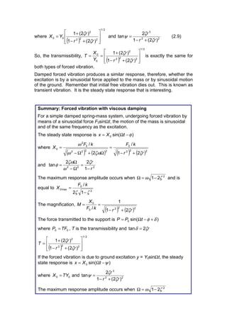
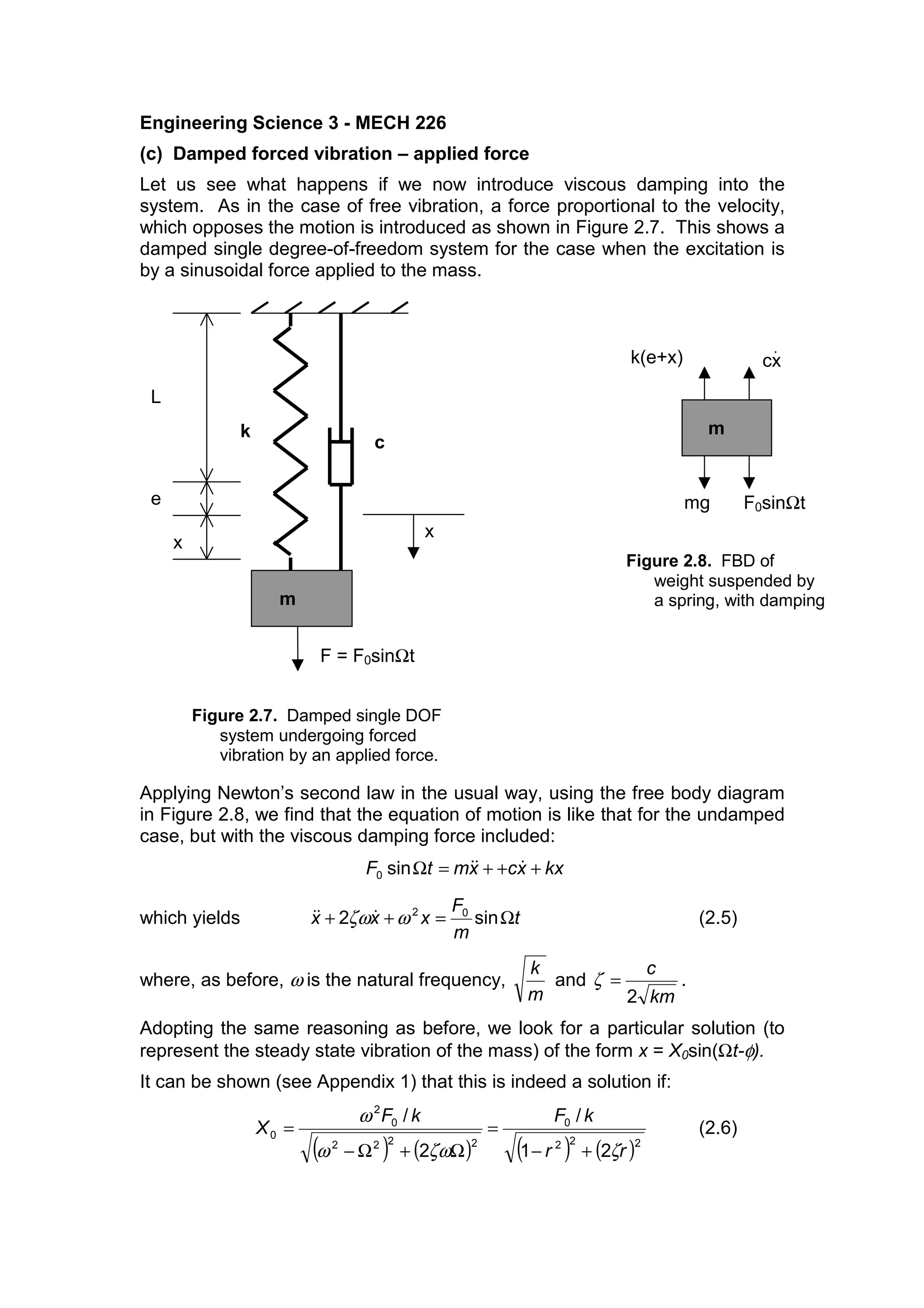
For a damped spring-mass system undergoing forced vibration by a sinusoidal force or ground excitation, the steady state response is also sinusoidal at the excitation frequency. The maximum response amplitude occurs at a frequency slightly below the natural frequency and decreases with increased damping. Damping reduces the sharpness of resonance and limits the maximum response amplitude reached.

1. Engineering Science 3 - MECH 226
(c) Damped forced vibration – applied force
Let us see what happens if we now introduce viscous damping into the
system. As in the case of free vibration, a force proportional to the velocity,
which opposes the motion is introduced as shown in Figure 2.7. This shows a
damped single degree-of-freedom system for the case when the excitation is
by a sinusoidal force applied to the mass.
Applying Newton’s second law in the usual way, using the free body diagram
in Figure 2.8, we find that the equation of motion is like that for the undamped
case, but with the viscous damping force included:
kxxcxmtF +++=Ω sin0
which yields t
m
F
xxx Ω=++ sin2 02
ωζω (2.5)
where, as before, ω is the natural frequency,
m
k
and
km
c
2
=ζ .
Adopting the same reasoning as before, we look for a particular solution (to
represent the steady state vibration of the mass) of the form x = X0sin(Ωt-φ).
It can be shown (see Appendix 1) that this is indeed a solution if:
( ) ( ) ( ) ( )222
0
2222
0
2
0
21
/
2
/
rr
kFkF
X
ζζωω
ω
+−
=
Ω+Ω−
= (2.6)
x
k
m
c
F = F0sinΩt
L
e
x
Figure 2.8. FBD of
weight suspended by
a spring, with damping
Figure 2.7. Damped single DOF
system undergoing forced
vibration by an applied force.
m
k(e+x)
mg F0sinΩt
cx
.

2. and 222
1
22
tan
r
r
−
=
Ω−
Ω
=
ζ
ω
ζω
φ (2.7)
The way that the response amplitude X0 varies with the driving frequency is
shown in Figure 2.9 where X0 is plotted against the non-dimensional
frequency r, which is directly proportional to the driving frequency. In Figure
2.10 the phase angle φ is plotted against r, where the phase angle has been
calculated in degrees. It can also be measured in radians (π radians = 180°).
Curves are shown for different values of ζ to illustrate the effect on the
response of the amount of damping in the system.
These results show up some interesting trends, which are borne out in
practice. Firstly, we can see that the maximum response amplitude depends
on how much damping there is in the system. The less damping there is (i.e.
the smaller is ζ) the larger it gets, and if there is no damping at all, then the
maximum amplitude possible is infinite, as we saw earlier.
0 0.5 1 1.5 2 2.5 3
Frequency ratio, r
Responseamplitude,X0
ζ = 0.01
ζ = 1
ζ = 0.05
ζ = 0.1
Figure 2.9. The
response
amplitude of a
damped
system with
an applied
force as a
function of the
frequency
ratio
Figure 2.10.
The phase
angle of a
damped
system with
an applied
force as a
function of the
frequency
ratio
0
30
60
90
120
150
180
0 0.5 1 1.5 2 2.5 3
Frequency ratio, r
Phaseangle,φφφφ

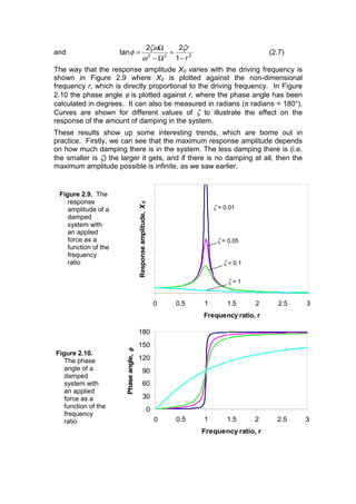
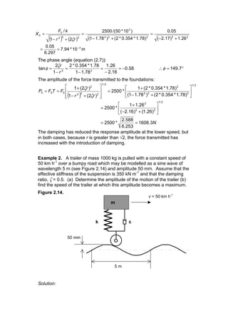
3. It is clear, too, that the more damping there is, the more slowly does the
amplitude build up to its maximum as the driving frequency is increased. At
low damping, there is a sudden increase in amplitude as the driving frequency
approaches the natural frequency, and a sudden drop in amplitude as r
becomes bigger than 1. While, as the damping is increased, the build up to
the maximum amplitude is much more gradual, and “resonance” becomes
less sharp.
We can see that at very low driving frequencies (small r), the amplitude of the
response is almost the same as the static displacement, F0/k, but at very high
driving frequencies (large r), the amplitude tends to become zero, no matter
how little damping there is. The system simply doesn’t have time to respond.
You may not be able to see very clearly from Figure 2.9 that the maximum
amplitude of the response does not occur when r = 1, as it did for the
undamped system. From equation (2.6) it should be clear that X0 will be a
maximum when the denominator [(1-r2
)2
+ (2ζr)2
] is a minimum. To find the
value of r at which this occurs, we need to differentiate with respect to r (see
Appendix 1). We find that the amplitude becomes a maximum when
2
21 ζ−=r or 2
21 ζω −=Ω . For small ζ, the maximum occurs when r ≈ 1,
but if the system has high damping, then the frequency at which the response
becomes a maximum is lower than the natural frequency.
Once again, we see that a driving frequency near to the natural frequency
produces rather critical conditions, and if excessive amplitudes are to be
avoided, then driving the system close to its resonant frequency is to be
avoided. This means that either the system should be driven at a different
frequency or the stiffness, k, or mass, m, should be altered to change the
natural frequency, ω.
We can observe from Figure 2.10 that when the driving frequency is low, the
response is very nearly in phase with the excitation, shown by a small value of
φ, but when the frequency is high, the response is 180° out of phase (exactly
out of phase), while at r = 1, when the driving frequency is exactly the same
as the natural frequency, the response is 90° out of phase. So, as the
frequency is gradually increased, the response will change from being in
phase at frequencies below the resonant frequency to being out of phase at
frequencies above it. If the damping in the system is low, this change is very
sudden, and can readily be observed experimentally. As the damping is
increased, the change becomes more gradual. With critical damping (ζ = 1),
the change is very gradual, and the response becomes exactly out of phase
only at very high driving frequencies.
Note that the term “resonant frequency” is used sometimes to denote the
frequency at which the response amplitude becomes a maximum, and
sometimes the frequency at which r = 1. For low damping, the two are very
nearly the same, but for highly damped systems it should be made clear
which definition is used. In this course, I will stick to the definition of resonant
frequency as that for which r = 1, so that the resonant frequency and the
undamped natural frequency are the same, while the frequency at which the
amplitude becomes a maximum is 2
21 ζω − .

4. The magnification, M, as in the previous section, is:
( ) ( )2220
0
21
1
/ rrkF
X
M
ζ+−
==
So a plot of M against r will give the same result as shown in Figure 2.9 if F0/k
= 1.
The transmissibility, defined above, T = P0/F0, where P0 is the amplitude of the
force transmitted to the support. With viscous damping, the force transmitted
is
)sin()cos( 00 φφ −Ω+−ΩΩ=+= tkXtXckxxcP
This can be shown (see Appendix 1) to be of the form: )sin(0 δφ +−Ω= tPP
where
( )
2/1
222
2
00
)2(1
)2(1
ú
ú
û
ù
ê
ê
ë
é
+−
+
=
rr
r
FP
ζ
ζ
and rζδ 2tan =
The transmissibility T is ,therefore
( )
2/1
222
2
)2(1
)2(1
ú
ú
û
ù
ê
ê
ë
é
+−
+
=
rr
r
T
ζ
ζ
This looks rather a complicated expression, but once you know ζ and r, it just
needs a bit of care putting the numbers into your calculator to come up with
the right answer. The way the transmissibility varies with r is shown in Figure
2.11.
As with the maximum response amplitude, the force transmitted to the support
becomes a maximum when 2
21 ζω −=Ω . The force transmitted is equal to
the driving force at Ω = √2ω. As the damping in the system is increased, the
magnitude of the force transmitted gets smaller as long as Ω √2ω, but when
Figure 2.11. The transmissibility
of a damped single DOF
system as a function of the
frequency ratio.
0
1
2
3
4
5
6
0 0.5 1 1.5 2 2.5 3
Frequency ratio, r
Transmissibility,T
ζ = 0.01
ζ = 0.2
ζ = 0.5
ζ = 1

5. the drive frequency is higher than this, the effect of increasing the damping is
reversed.
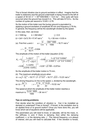
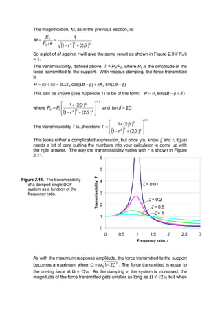
(d) Damped forced vibration – ground excitation
You should be familiar now with the way to set about looking at these
problems, so Figure 2.12 which shows a damped single degree-of-freedom
system undergoing forced vibration by means of ground excitation should
come as no surprise to you. Figure 2.13 shows the free body diagram of the
mass, and the equation of motion is derived exactly in the way we have used
before, by applying Newton’s second law. The results are given below.
The equation of motion: ( )[ ] xmyxcyxekmgFx
=−−−+−=å )(
kxxcxmycky ++=+∴
Dividing all through by m, and rewriting:
tY
m
c
tY
m
k
x
m
k
x
m
c
x Ω
Ω
+Ω=++ cossin 00
tYtYxxx ΩΩ+Ω=++∴ cos2sin2 00
22
ζωωωζω (2.8)
where, as before, ω is the natural frequency,
m
k
and
km
c
2
=ζ .
It can be shown (see Appendix 1) that this has the particular solution:
)sin(0 ψ−Ω= tXx
x
k
m
c
y = Y0sinΩt
L
e
x
m
k[e+(x-y)]
mg
)( yxc −
Figure 2.13. FBD of
weight suspended by
a spring, with damping
Figure 2.12. Forced vibration of a
damped single DOF system by ground
excitation

6. where
( )
2/1
222
2
00
)2(1
)2(1
ú
ú
û
ù
ê
ê
ë
é
+−
+
=
rr
r
YX
ζ
ζ
and 22
3
)2(1
2
tan
rr
r
ζ
ζ
ψ
+−
= (2.9)
So, the transmissibility,
( )
2/1
222
2
0
0
)2(1
)2(1
ú
ú
û
ù
ê
ê
ë
é
+−
+
==
rr
r
Y
X
T
ζ
ζ
is exactly the same for
both types of forced vibration.
Damped forced vibration produces a similar response, therefore, whether the
excitation is by a sinusoidal force applied to the mass or by sinusoidal motion
of the ground. Remember that initial free vibration dies out. This is known as
transient vibration. It is the steady state response that is interesting.
Summary: Forced vibration with viscous damping
For a simple damped spring-mass system, undergoing forced vibration by
means of a sinusoidal force F0sinΩt, the motion of the mass is sinusoidal
and of the same frequency as the excitation.
The steady state response is )sin(0 φ−Ω= tXx
where
( ) ( ) ( ) ( )222
0
2222
0
2
0
21
/
2
/
rr
kFkF
X
ζζωω
ω
+−
=
Ω+Ω−
=
and 222
1
22
tan
r
r
−
=
Ω−
Ω
=
ζ
ω
ζω
φ
The maximum response amplitude occurs when 2
21 ζω −=Ω and is
equal to
2
0
max0
12
/
ζζ −
=
kF
X
The magnification,
( ) ( )2220
0
21
1
/ rrkF
X
M
ζ+−
==
The force transmitted to the support is )sin(0 δφ +−Ω= tPP
where 00 TFP = , T is the transmissibility and rζδ 2tan =
( )
2/1
222
2
)2(1
)2(1
ú
ú
û
ù
ê
ê
ë
é
+−
+
=
rr
r
T
ζ
ζ
If the forced vibration is due to ground excitation y = Y0sinΩt, the steady
state response is )sin(0 ψ−Ω= tXx
where 00 TYX = and 22
3
)2(1
2
tan
rr
r
ζ
ζ
ψ
+−
=
The maximum response amplitude occurs when 2
21 ζω −=Ω

7. The effect of damping is to limit the maximum response amplitude and to
reduce the sharpness of resonance, which can be defined as occurring
when the drive frequency Ω equals the natural frequency of the system, ω.
Example 4. Consider the machine of Example 3, where viscous damping has
now been introduced such that damping coefficient, c is 5 kNm-1
. Calculate
the response amplitude, the phase angle, and the force transmitted to the
foundations when the driving frequency is (a) 20 Hz and (b) 2 Hz. The
amplitude of the applied force is, as before, 2500 N.
Solution:
This is a case of damped forced vibration due to an applied force.
(a) As before: m = 1000 kg F0 = 2500 N c = 5 kNm-1
Ω = 20 Hz = 2π*20 = 125.7 rad s-1
k = 50 kNm-1
.
The natural frequency ω = 7.07 rad s-1
and r = 17.8
(a) The damping ratio, 354.0
1000*10*502
10*5
2 3
3
===
km
c
ζ
The response amplitude (equation (2.6)):
( ) ( )
m
rr
kF
X
4
22222
3
222
0
0
10*58.1
1.316
05.0
6.12)84.315(
05.0
)8.17*354.0*2()8.171(
)10*50/(2500
21
/
−
==
+−
=
+−
=
+−
=
ζ
So the response amplitude is still very small at less than 0.16 mm.
The phase angle (equation (2.7)):
04.0
84.315
6.12
8.171
8.17*354.0*2
1
2
tan 22
−=
−
=
−
=
−
=
r
rζ
φ °=∴ 7.177φ
The amplitude of the force transmitted to the foundations:
( )
N
rr
r
FTFP
100
7.99913
76.159
*2500
)6.12()84.315(
6.121
*2500
)8.17*354.0*2()8.171(
)8.17*354.0*2(1
*2500
)2(1
)2(1
2/1
22
2
2/1
222
2
2/1
222
2
000
==
ú
û
ù
ê
ë
é
+−
+
=
ú
û
ù
ê
ë
é
+−
+
=
ú
ú
û
ù
ê
ê
ë
é
+−
+
==
ζ
ζ
The force transmitted to the foundations is therefore increased by the
introduction of damping.
(b) Ω = 2 Hz = 2π*2 = 12.57 rad s-1
and r = 1.78

8. ( ) ( )
m
rr
kF
X
3
22222
3
222
0
0
10*94.7
297.6
05.0
26.1)17.2(
05.0
)78.1*354.0*2()78.11(
)10*50/(2500
21
/
−
==
+−
=
+−
=
+−
=
ζ
The phase angle (equation (2.7)):
58.0
16.2
26.1
78.11
78.1*354.0*2
1
2
tan 22
−=
−
=
−
=
−
=
r
rζ
φ °=∴ 7.149φ
The amplitude of the force transmitted to the foundations:
( )
N
rr
r
FTFP
3.1608
253.6
588.2
*2500
)26.1()16.2(
26.11
*2500
)78.1*354.0*2()78.11(
)78.1*354.0*2(1
*2500
)2(1
)2(1
2/1
22
2
2/1
222
2
2/1
222
2
000
==
ú
û
ù
ê
ë
é
+−
+
=
ú
û
ù
ê
ë
é
+−
+
=
ú
ú
û
ù
ê
ê
ë
é
+−
+
==
ζ
ζ
The damping has reduced the response amplitude at the lower speed, but
in both cases, because r is greater than √2, the force transmitted has
increased with the introduction of damping.
Example 2. A trailer of mass 1000 kg is pulled with a constant speed of
50 km h-1
over a bumpy road which may be modelled as a sine wave of
wavelength 5 m (see Figure 2.14) and amplitude 50 mm. Assume that the
effective stiffness of the suspension is 350 kN m-1
and that the damping
ratio, ζ = 0.5. (a) Determine the amplitude of the motion of the trailer (b)
find the speed of the trailer at which this amplitude becomes a maximum.
Figure 2.14.
Solution:
5 m
k
m
c
50 mm
v = 50 km h-1

9. This is forced vibration due to ground excitation in effect. Imagine that the
trailer is stationery and the ground underneath is being moved to the left at
a speed of 50 km h-1
= 50*1000/3600 = 13.9 ms-1
. One cycle will have
occurred when the ground has moved 5 m. This will take 5/13.9 s. So the
number of cycles per second is 13.9/5 = 2.78.
So the motion of the trailer over the bumpy ground is equivalent to
applying a ground excitation of amplitude 50 mm and frequency 2.78 Hz.
In general, the frequency will be the wavelength divided by the speed.
In this case, then, we know:
m = 1000 kg k = 350 kNm-1
ζ = 0.5
Ω = 2πf = 2π*2.78 =17.47 rad s-1
Y0 = 50 mm = 0.05 m
(a) First find ω and r: 71.18
1000
1000*350
===
m
k
ω rad s-1
934.0
71.18
47.17
==
Ω
=∴
ω
r
The amplitude of the motion of the trailer (equation (2.9))
( )
m
rr
r
YX
073.0108.2*05.0
872.0016.0
872.01
05.0
)934.0*5.0*2()934.01(
)934.0*5.0*2(1
05.0
)2(1
)2(1
2/1
2/1
222
2
2/1
222
2
00
==ú
û
ù
ê
ë
é
+
+
=
ú
û
ù
ê
ë
é
+−
+
=
ú
ú
û
ù
ê
ê
ë
é
+−
+
=
ζ
ζ
So the amplitude of the trailer motion is 73 mm.
(b) The maximum amplitude occurs when
23.135.0*71.185.0*21*71.1821 22
==−=−=Ω ζω rad s-1
The driving frequency (in Hz) is the speed, v, divided by the wavelength,
so
5
*2 vπ
=Ω 53.10
2
23.13*5
2
*5
==
Ω
=∴
ππ
v ms-1
The speed at which the amplitude of the trailer motion reaches a
maximum is 38
1000
3600*53.10
= km h-1
Tips on solving problems
First decide what the condition of vibration is. Can it be modelled as
damped or undamped? Free or forced? If forced, is the excitation due to
an applied force or to ground motion? Once you have done this, you will
know which set of equations will be applicable.
The parameters you will need to know, or calculate, will be the mass, m,
the stiffness, k, and, if there is damping, then either the damping
coefficient, c, or the damping ratio, ζ. The natural frequency ω is always
of interest, and you will need to calculate that. If the vibration is forced,

10. then the excitation frequency Ω will need to be known, and, hence, the
frequency ratio, r can be determined. Armed with these parameters, the
response of the system (how it behaves in terms of its displacement from
the equilibrium position) can be resolved.
Measurement of vibration
An accelerometer is a piezo-electric device that is frequently used to
monitor vibration. It is attached rigidly to the system of interest, such as a
wing of an aircraft under test. It measures the acceleration at the point
where it is attached, giving a voltage output that is directly proportional to
the acceleration. This voltage can be integrated by suitable electronic
instrumentation to provide values of velocity and displacement. The use
of an amplifier and an oscilloscope or a frequency meter allows the
frequency of vibration to be determined. To determine the undamped
natural frequency, the object of interest, an engine perhaps, should be
supported as freely as possible, because any sources of friction will
introduce damping. If it is then given a light tap, or a small initial
displacement, and released it will vibrate at its natural frequency, which
can be determined from the accelerometer output. Ideally, the
accelerometer should have a small mass compared with the object under
test, although the extra mass can be taken into account.