Using a Common Theme to Find Intersections of Spheres with Lines and Planes via Geometric (Clifford) Algebra
•
2 likes•349 views

After reviewing the sorts of calculations for which Geometric Algebra (GA) is especially convenient, we identify a common theme through which those types of calculations can be used to find the intersections of spheres with lines, planes, and other spheres.
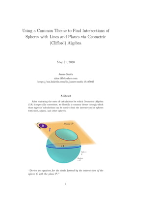
![Figure 1: An example of a problem statement: “Derive an equation for the circle
formed by the intersection of the sphere S with the plane P.”
1 Introduction
This document uses ideas that are explained more fully in [1] and [2]. Especially,
the symbol for a vector (for example, p, in Fig. 1) may be used to refer either to
the vector itself, or to its endpoint. In each such instance, we rely upon context
to make the intended meaning clear.
2 Example of a Problem Statement
“Derive an equation for the circle formed by the intersection of the
sphere S with the plane P (Fig. 1).”
3 A Review of Calculations for which Geomet-
ric Algebra (GA) is Especially Convenient
This brief review will—we hope —give us some ideas of what to “look for” when
we attempt to derive equations for intersections of spheres with other objects.](data:image/gif;base64,R0lGODlhAQABAIAAAAAAAP///yH5BAEAAAAALAAAAAABAAEAAAIBRAA7)
Recommended
Recommended
More Related Content
What's hot
What's hot (20)
Similar to Using a Common Theme to Find Intersections of Spheres with Lines and Planes via Geometric (Clifford) Algebra
Similar to Using a Common Theme to Find Intersections of Spheres with Lines and Planes via Geometric (Clifford) Algebra (20)
More from James Smith
More from James Smith (20)
Recently uploaded
Recently uploaded (20)
Using a Common Theme to Find Intersections of Spheres with Lines and Planes via Geometric (Clifford) Algebra
- 1. Using a Common Theme to Find Intersections of Spheres with Lines and Planes via Geometric (Clifford) Algebra May 21, 2020 James Smith nitac14b@yahoo.com https://mx.linkedin.com/in/james-smith-1b195047 Abstract After reviewing the sorts of calculations for which Geometric Algebra (GA) is especially convenient, we identify a common theme through which those types of calculations can be used to find the intersections of spheres with lines, planes, and other spheres. “Derive an equation for the circle formed by the intersection of the sphere S with the plane P.” 1
- 2. Figure 1: An example of a problem statement: “Derive an equation for the circle formed by the intersection of the sphere S with the plane P.” 1 Introduction This document uses ideas that are explained more fully in [1] and [2]. Especially, the symbol for a vector (for example, p, in Fig. 1) may be used to refer either to the vector itself, or to its endpoint. In each such instance, we rely upon context to make the intended meaning clear. 2 Example of a Problem Statement “Derive an equation for the circle formed by the intersection of the sphere S with the plane P (Fig. 1).” 3 A Review of Calculations for which Geomet- ric Algebra (GA) is Especially Convenient This brief review will—we hope —give us some ideas of what to “look for” when we attempt to derive equations for intersections of spheres with other objects.
- 3. Figure 2: The projection v u and rejection (v⊥u) of the vector v with respect to vector w. Figure 3: The projection v ˆB and rejection v⊥ ˆB of the vector v with respect to bivector ˆB. 3.1 Projections and “Rejections” of Vectors The projection and “rejection” of a vector v with respect to a vector w (Fig. 2) are given by v w = (v · w) w−1 = (v · ˆw) ˆw and v⊥w = (v ∧ w) w−1 = (v ∧ ˆw) ˆw. Please recall that vectors do not possess the attribute of location. Therefore, the components of v parallel and perpendicular to w are the same no matter where we draw v. We can also find the projection and rejection of a vector with respect to a bivector. Note that ˆB −1 = − ˆB: 3
- 4. Figure 4: Equation for a circle in a plane parallel to the bivector ˆB in a two-dimensional case. v ˆB = v · ˆB ˆB −1 = − v · ˆB ˆB and v⊥ ˆB = v ∧ ˆB ˆB −1 = − v ∧ ˆB ˆB. 3.2 Designating Circles via Rotation of Vectors The equation that we gave for a circle in two-dimensional GA (4) can be extended to 3D (Fig. 5) 4 A Simple Problem that will Provide the Pat- tern that We Seek To find the points at which a circle is intersected by a line through point P with direction ˆu (Fig. 6) can be found by using the ideas from Fig. 2 (Fig. 7) We will seek to transform the problems that follow into ones in which the unknowns are point of intersection between a line and a circle. 4
- 5. Figure 5: Extension to 3D, of the equation shown in Fig. 4. The red circle is in a plane parallel to the bivector ˆB. The circle’s equation can be written as x = c + (p − c) eθ ˆB . Figure 6: A Simple problem that will provide the pattern that we seek: Find the points at which a circle is intersected by a line through point p with direction ˆu. 5
- 6. Figure 7: The points of intersection found by using the ideas shown in Fig. 2 : x1 = c + (p − c)⊥ˆu − ˆu r2 − [(p − c))⊥ˆu] 2 ; x2 = c + (p − c)⊥ˆu + ˆu r2 − [(p − c))⊥ˆu] 2 . 5 “Seeing” Our Simple Pattern in Other Inter- section Problems 5.1 Intersection of a Line with a Sphere Our pattern is easy to “see” in our first problem: the intersection of a line with a sphere (Fig. 8). We just introduce the circle whose center is s, and that passes through the two points of intersection (Fig. 9). 5.2 Intersection of a Line with a Sphere The intersection of a plane with a sphere is a circle (Fig. 10). We’ll call that circle the “solution circle”. If we can identify any point on that circle, then we can give the equation of that circle in the form described in connection with Fig. 5. To identify such a point, we’ll use an additional idea from our review of things for which GA is especially convenient: we can find the projection of the vector (p − s) upon the plane (Fig. 11). The line that has that direction, and that passes through point p, also passes through the center of the solution circle (because that center is the projection of the point s upon the plane). Therefore, that line intersects the solution circle—and by extension, the given sphere —in two points (Fig. 12. Now, we can find one of those points (q , in Fig. 12)via the method we used to find the points of intersection of a line with a sphere. 6
- 7. Figure 8: How can we “see” our pattern in the case of a line intersecting a sphere? Figure 9: By adding to Fig. 8 the red circle (through the two points of intersection, with center s, we transform this problem into the one we treated in Figs. 6 and 7. 7
- 8. Figure 10: Our second problem: Give the equation for the circle of intersection between a given plane and sphere. Figure 11: Making use of one idea that we noted in our review of things for which GA is convenient, we’ll add the line that goes through point p, and that has the direction of vector (p − s)’s projection upon the plane. 8
- 9. Figure 12: The line that has the direction (p − s), and that passes through point p, also passes through the center of the solution circle (because that center is the projection of the point s upon the plane). Therefore, that line intersects the solution circle—and by extension, the given sphere —in two points. Now, we can find one of those points (here, q) via the method we used for finding the points of intersection of a line with a sphere. Figure 13: Having identified one point (q) on the solution circle, we can write the equation of that circle as x = s + (q − s) eθ ˆB . 9
- 10. Figure 14: Our third problem: to find the intersection (circle C) of the two spheres, we will look for elements that will enable us to transform this problem into a combination of those which we have already solved. 5.3 Intersection of Two Spheres The intersection of two spheres is a circle (C, in Fig. 14). Before plunging into GA, let’s see what else we might notice or deduce. One key feature is that the solution circle is perpendicular to the line that joins the centers of the given spheres. Put differently, the solution circle’s center (point c in Fig. 15) is at some distance d from point s1, in the direction given by the vector (s2 − s1). We can calculate that distance by equating two expressions for the solution circle’s radius: R2 1 − d2 = R2 2 − ( s2 − s1 − d) 2 ∴ d = R2 1 − R2 2 + s2 − s1 2 / [2 s2 − s1 ] . We’ve now located point c, which (very importantly, for our purposes) is a point on the plane that contains the solution circle. What else might we need, in order to transform this problem into one similar to those that we have already solved? Possibilities include (1) the bivector of the plane that contains the solution circle, and (2) a point on that circle. Finding a unit bivector ˆM of a plane perpendicular to given unit vector ˆw 10
- 11. Figure 15: Based upon previous experience, we try to identify a point that lies on the plane of C. Here, we use point c, which is the center of that circle. The vector (c − s1) has the direction of (s2 − s1), and length R2 1 − R2 2 + s2 − s1 2 / [2 s2 − s1 ] . 11
- 12. Figure 16: Identifying another element that should prove useful: a unit bivector for the plane that contains C . (Please recall that the two unit bivectors for a given plane differ only in their signs.) The unit bivector that we’ve chosen is the dual of the unit vector in the direction of (s2 − s1). Specifically, ˆB = s2 − s1 s2 − s1 I3. is another thing that can be done conveniently via GA: ˆM = ˆwI3 where I3 (= e1e2e3) is the unit pseudoscalar for three-dimensional GA ([1], pp. 105-107). Therefore, a unit bivector ˆB (Fig. 16) of the plane that contains the solution circle is ˆB = s2 − s1 s2 − s1 I3 . (Please recall that the two unit bivectors for a given plane differ only in their signs.) Now that we’ve identified ˆB, we can make use, again, of experiences from previous problems by identifying a line that intersects the solution circle in a point that we will be able to identify. Here, that line is the one that passes through point c, and has the direction of c ˆB. We’ve now arrived at the “intersection of line and sphere” problem (Fig. 17). Therefore, we add the vectors from point s1 to the two points of intersection (Fig. 18). For our purposes, we need to find only one point (q, in Fig. 19) of intersection of the line with the spheres. Having done so, we can write the equation of C as x = s1 + (q − s1) eθ ˆB . 12
- 13. Figure 17: Now that we’ve identified ˆB we can make use, again, of experiences from previous problems by identifying a line that intersects the solution circle in a point that we will be able to identify. Here, that line is the one that passes through point c, and has the direction of c ˆB. We’ve now arrived at the “intersection of line and sphere” problem. Figure 18: In Fig. 17, we arrived at the “intersection of line and sphere” problem. Therefore, we add the vectors from point s1 to the two points of intersection. 13
- 14. Figure 19: For our purposes, we need to find only one point (q) of intersection of the line with the spheres. Rotation of the vector (q − s1) with respect to ˆB gives C. Figure 20: Now, we can write the equation of C as x = s1 + (q − s1) eθ ˆB . 14
- 15. References [1] A. Macdonald, Linear and Geometric Algebra (First Edition), CreateSpace Independent Publishing Platform (Lexington, 2012). [2] J. Smith, 2016, “Some Solution Strategies for Equations that Arise in Geometric (Clifford) Algebra”, http://vixra.org/abs/1610.0054. 15