This document summarizes an implementation of curve subdivision schemes including B-splines, four point subdivision, and J-splines. It compares the properties of these schemes and describes an approach for implementing them using subdivision, where new points are calculated as a weighted sum of previous points. It also describes implementing parallel transport of vectors along a curve and compensating for the accumulated angle defect by spreading the defect across the curve. The output is an interactive demo visualizing these techniques.

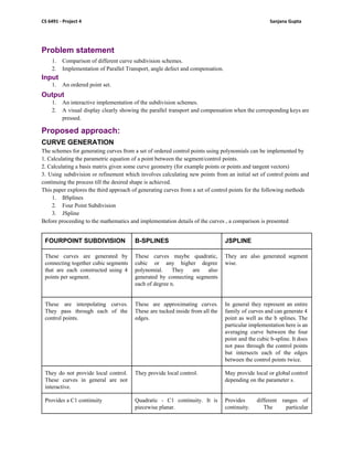
1. CS 6491 - Project 4 Sanjana Gupta
Problem statement
1. Comparison of different curve subdivision schemes.
2. Implementation of Parallel Transport, angle defect and compensation.
Input
1. An ordered point set.
Output
1. An interactive implementation of the subdivision schemes.
2. A visual display clearly showing the parallel transport and compensation when the corresponding keys are
pressed.
Proposed approach:
CURVE GENERATION
The schemes for generating curves from a set of ordered control points using polynomials can be implemented by
1. Calculating the parametric equation of a point between the segment/control points.
2. Calculating a basis matrix given some curve geometry (for example points or points and tangent vectors)
3. Using subdivision or refinement which involves calculating new points from an initial set of control points and
continuing the process till the desired shape is achieved.
This paper explores the third approach of generating curves from a set of control points for the following methods
1. BSplines
2. Four Point Subdivision
3. JSpline
Before proceeding to the mathematics and implementation details of the curves , a comparison is presented
FOURPOINT SUBDIVISION B-SPLINES JSPLINE
These curves are generated by
connecting together cubic segments
that are each constructed using 4
points per segment.
These curves maybe quadratic,
cubic or any higher degree
polynomial. They are also
generated by connecting segments
each of degree n.
They are also generated segment
wise.
These are interpolating curves.
They pass through each of the
control points.
These are approximating curves.
These are tucked inside from all the
edges.
In general they represent an entire
family of curves and can generate 4
point as well as the b splines. The
particular implementation here is an
averaging curve between the four
point and the cubic b-spline. It does
not pass through the control points
but intersects each of the edges
between the control points twice.
They do not provide local control.
These curves in general are not
interactive.
They provide local control. May provide local or global control
depending on the parameter s.
Provides a C1 continuity Quadratic - C1 continuity. It is
piecewise planar.
Provides different ranges of
continuity. The particular

2. CS 6491 - Project 4 Sanjana Gupta
Cubic - C2 continuity
Quintic - C4 continuity
implementation here gives a C2
continuity
This figure displays the 3 curves for the purpose of comparison. Green - Four Point , Blue - JSpline , Red -
Cubic B Spline.(The grey line is the polyline connecting the four points of the rectangle).
IMPLEMENTATIONS
A) SUBDIVISION SCHEMES
The idea behind generation via subdivision is calculating new points from an initial set of control points and
continuing the process till the desired shape is achieved.
i.e,
Each point P​k​
j​ is calculated as a weighted sum of the points P​k-1​
i ​of the previous iteration.

3. CS 6491 - Project 4 Sanjana Gupta
Therefore
P​k​
j ​= ∑​nk-1​
i=0 ​a​ijk ​ P​k-1​
j
Now for ​Uniform Quadratic B-Spline​ :
​P​2j​ = 0.75* P​j ​+ 0.25 * P​j+1
P​2j+1​ = 0.25* P​j​ + 0.75 * P​j+1
​The remaining 4 curves , namely , four point , cubic b spline, quintic b spline and j spline are all derived
from a single method as described in the J-Splines paper as follows:
k+1​
P​2j​ = (a ​k​
P​j–1​ + (8–2a) ​k​
P​j​ + a ​k​
P​j+1​)/8
k+1​
P​2j+1​
= ((b–1) ​k​
P​j–1​ + (9–b)​ k​
P​j​ + (9–b) ​k​
P​j+1​ + (b–1) ​k​
P​j+2​)/16
Setting a = b = (say) s we get:
Four Point Subdivision for s = 0
As:
P​2j​ = P​j
P​2j+1​ = (-1.0/16) * P​j-1​ + (9.0/16) * P​j​ +(9.0/16) * P​j+1​ +(1.0/16) P​j+2
Cubic B Spline for s = 1
​P​2j​ = (1.0/8) * P​j-1 ​+0.75* P​j ​+(1.0/8) * P​j+1
​P​2j+1​ = 0.5* P​j ​+ 0.5 * P​j+1
J Spline for s = 0.5
​P​2j​ =(1.0/16) * P​j-1 ​+ (7.0/8) * P​j ​+(1.0/16) * P​j+
P​2j+1​ = (-1.0/32) * P​j-1​ + (17.0/32) * P​j​ +(17.0/32) * P​j+1​ +(-1.0/32) P​j+2
Quintic B Spline for s = 1.5
​P​2j​ = (1.5/8) * P​j-1 ​+ (5.0/8) * P​j ​+ (1.5/8) * P​j+
P​2j+1​ = (1.0/32) * P​j-1​ + (7.5/16) * P​j​ +(7.5/16) * P​j+1​ +(1.0/32) P​j+2
B) PARALLEL TRANSPORT AND COMPENSATION
The notion of parallel transport is the idea of translating a ​vector field along a ​differentiable ​curve to
attain a new vector field which is ​parallel​ to .
To realise the parallel transport and compensation, the following 4 steps are implemented:
1. A starting normal W = N​0 is calculated as max(in magnitude) of V(P​0​,P​1​) X V(1,0,0) and
V(P​0​,P​1​) X V(0,1,0).

4. CS 6491 - Project 4 Sanjana Gupta
2. Then each of N​i ​is calculated recursively from N​i-1 ​using the following scheme:
2.1. For N​i-1 ​a local coordinate frame is calculated. The normal to the triangle formed by P​i-1​,
P​i​, P​i+1 called N​ab forms one axis. The second axis of the coordinated frame , H​ab is
calculated as a cross product of N​ab​ and V(P​i-1​,P​i​).
2.2. The direction cosines x​i-1​ and y​i-1​ are calculated for N​0​ in this coordinate frame.
x​i-1​ = dot(N​i-1 ​,​ H​ab,​)
y​i-1​ = dot(N​i-1 ​,​​N​ab​)
2.3. The coordinate frame for N​i ​is then evaluated.The first axis N​bc​= N​ab​. ​The other axis, H​bc ​,
is calculated as the cross product of ​ N​bc​ and V(P​i​,P​i+1​).
2.4. Then N​i​ = x​i-1 ​H​bc ​+ y​i-1 ​N​bc
3. The angle defect is then calculated as the difference in angle between W and the N’​0 (the
calculated normal vector of P0 and P1). It is calculated as
angleDefect = atan2(dot(U’,V) , dot(U,V))
Where U = W
and U’ = cross(U , V(P​0​,P​1​))
4. Finally, this angle defect is spread across each of the calculated normal vectors by rotating each of
these by a factor of (i/n)*angleDefect, where n is the number of points and i goes from 0 to n.

5. CS 6491 - Project 4 Sanjana Gupta
These images show the parallelly transported vectors in orange and compensated vectors in blue.
Important notes for the interactive demo:
1. The images presented here are for the purpose of illustration and explaining a point. The
interactive demo can be found with the attached folder.
2. In the demo : the red ball simulated movement over the compensated vectors. Its path can be
made visible by pressing the key “+”.
3. The pink curve (when made visible by clicking “+”) shows the compensated vectors. The
compensated vectors themselves can be seen as cyan by pressing “>”.
4. The cyan curve shows the parallely transported vectors. (Made visible by pressing the key “}”).
The parallel vectors themselves can be seen as orange by pressing “<”.
5. Finally, the start parallel vector is shown in green . And the finally calculated one is shown in red.
On applying the compensation it should be black , meaning the compensation once spread across
the curve matches the final angle.