1 Data Compression Lec (3)
-
Coding
Methods
2 Data Compression Lec (3)
1-Run-Length Encoding
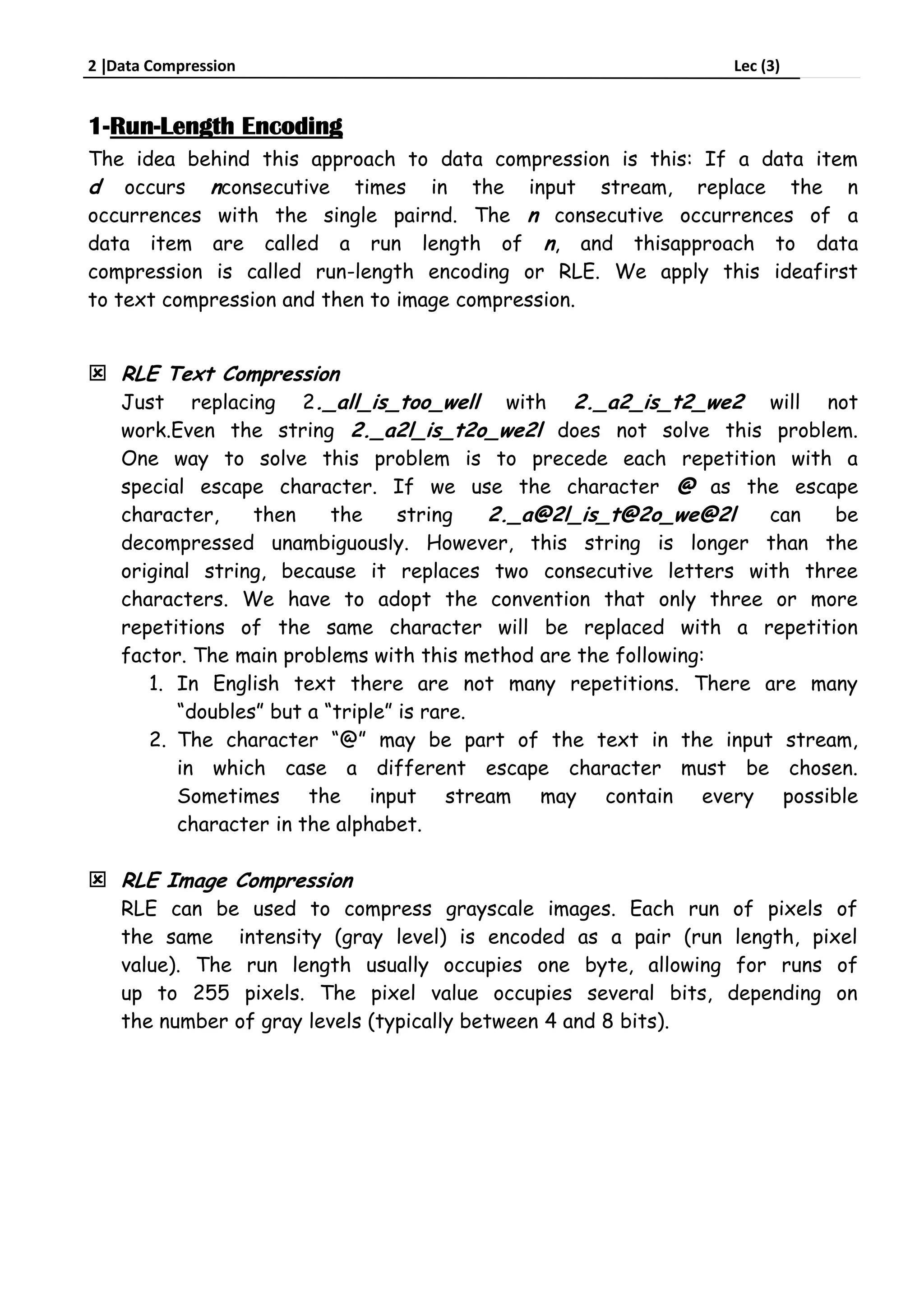
The idea behind this approach to data compression is this: If a data item
d occurs nconsecutive times in the input stream, replace the n
occurrences with the single pairnd. The n consecutive occurrences of a
data item are called a run length of n, and thisapproach to data
compression is called run-length encoding or RLE. We apply this ideafirst
to text compression and then to image compression.
 RLE Text Compression
Just replacing 2._all_is_too_well with 2._a2_is_t2_we2 will not
work.Even the string 2._a2l_is_t2o_we2l does not solve this problem.
One way to solve this problem is to precede each repetition with a
special escape character. If we use the character @ as the escape
character, then the string 2._a@2l_is_t@2o_we@2l can be
decompressed unambiguously. However, this string is longer than the
original string, because it replaces two consecutive letters with three
characters. We have to adopt the convention that only three or more
repetitions of the same character will be replaced with a repetition
factor. The main problems with this method are the following:
1. In English text there are not many repetitions. There are many
“doubles” but a “triple” is rare.
2. The character “@” may be part of the text in the input stream,
in which case a different escape character must be chosen.
Sometimes the input stream may contain every possible
character in the alphabet.
 RLE Image Compression
RLE can be used to compress grayscale images. Each run of pixels of
the same intensity (gray level) is encoded as a pair (run length, pixel
value). The run length usually occupies one byte, allowing for runs of
up to 255 pixels. The pixel value occupies several bits, depending on
the number of gray levels (typically between 4 and 8 bits).
3 Data Compression Lec (3)
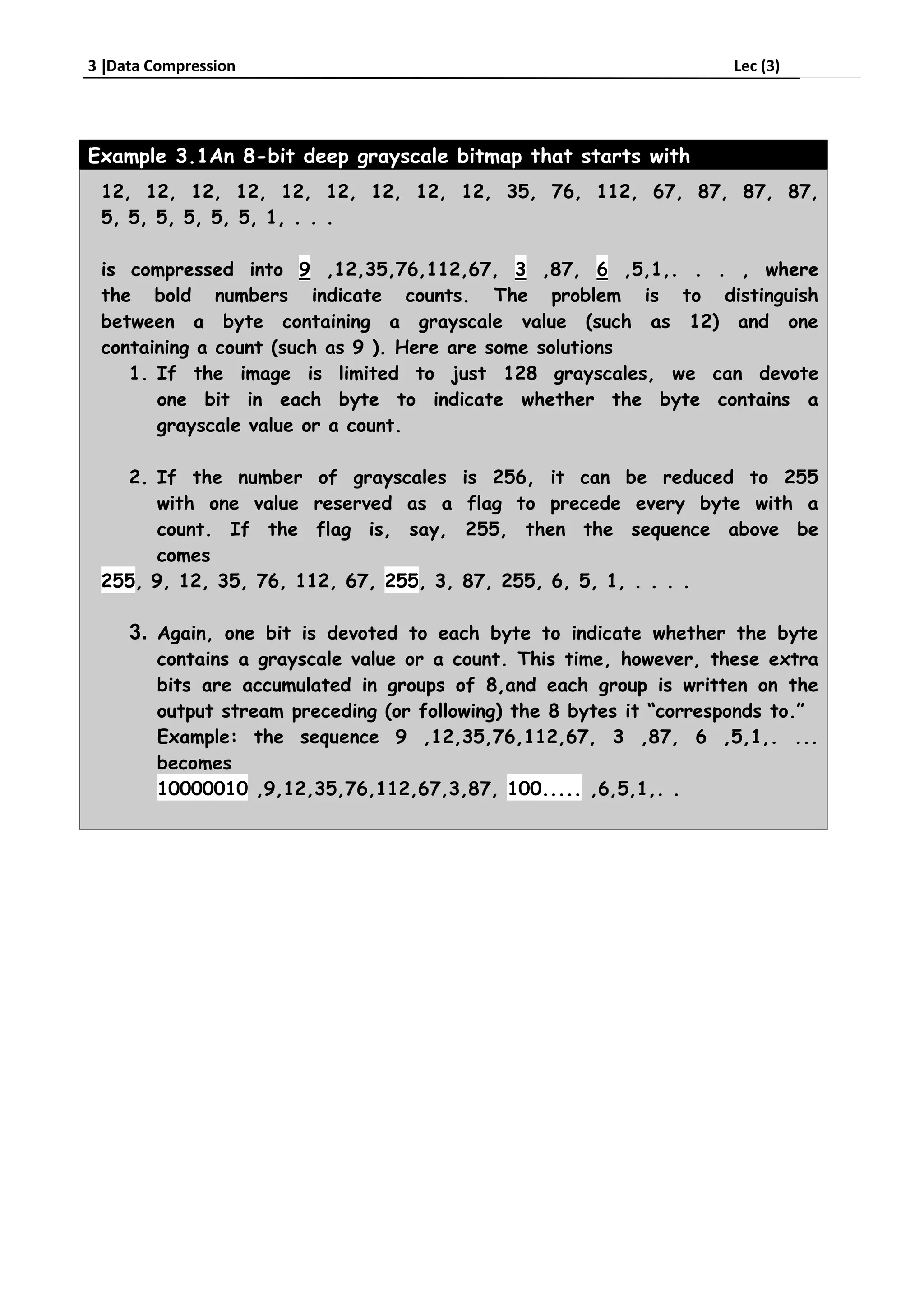
Example 3.1An 8-bit deep grayscale bitmap that starts with
12, 12, 12, 12, 12, 12, 12, 12, 12, 35, 76, 112, 67, 87, 87, 87,
5, 5, 5, 5, 5, 5, 1, . . .
is compressed into 9 ,12,35,76,112,67, 3 ,87, 6 ,5,1,. . . , where
the bold numbers indicate counts. The problem is to distinguish
between a byte containing a grayscale value (such as 12) and one
containing a count (such as 9 ). Here are some solutions
1. If the image is limited to just 128 grayscales, we can devote
one bit in each byte to indicate whether the byte contains a
grayscale value or a count.
2. If the number of grayscales is 256, it can be reduced to 255
with one value reserved as a flag to precede every byte with a
count. If the flag is, say, 255, then the sequence above be
comes
255, 9, 12, 35, 76, 112, 67, 255, 3, 87, 255, 6, 5, 1, . . . .
3. Again, one bit is devoted to each byte to indicate whether the byte
contains a grayscale value or a count. This time, however, these extra
bits are accumulated in groups of 8,and each group is written on the
output stream preceding (or following) the 8 bytes it “corresponds to.”
Example: the sequence 9 ,12,35,76,112,67, 3 ,87, 6 ,5,1,. ...
becomes
10000010 ,9,12,35,76,112,67,3,87, 100..... ,6,5,1,. .
4 Data Compression Lec (3)
2-Move-to-Front Coding
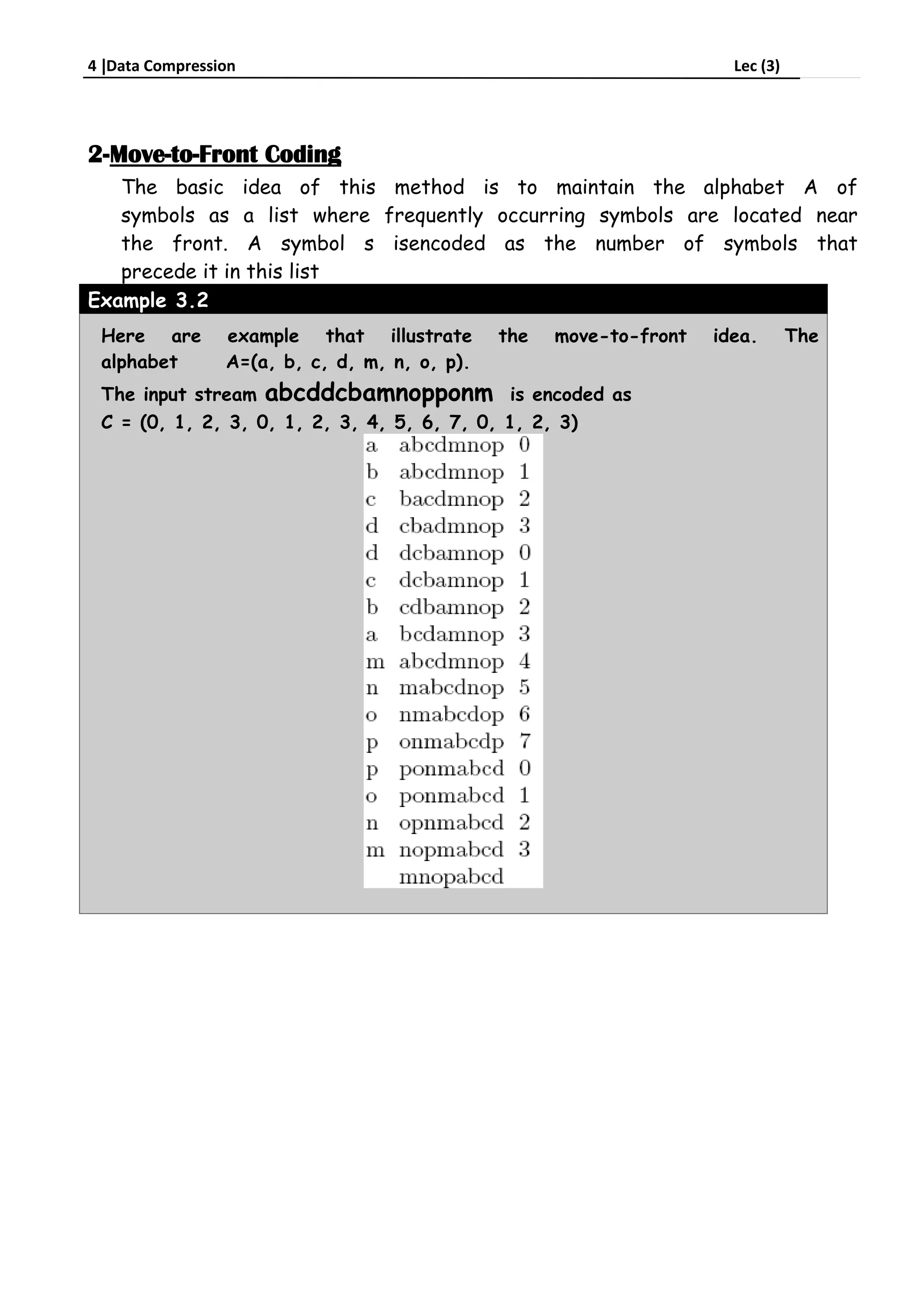
The basic idea of this method is to maintain the alphabet A of
symbols as a list where frequently occurring symbols are located near
the front. A symbol s isencoded as the number of symbols that
precede it in this list
Example 3.2
Here are example that illustrate the move-to-front idea. The
alphabet A=(a, b, c, d, m, n, o, p)
The input stream abcddcbamnopponm is encoded as
C = (0, 1, 2, 3, 0, 1, 2, 3, 4, 5, 6, 7, 0, 1, 2, 3)
5 Data Compression Lec (3)
3-Huffman coding
Huffman encoding is a way to assign binary codes to symbols that
reduces the overall number of bitsused to encode a typical string of
those symbols.
For example, if you use letters as symbols and have details of the
frequency of occurence of those letters in typical strings, then you
could just encode each letter with a fixed number of bits, such as in
ASCII codes. You can do better than this by encoding more
frequently occurring letters such as e and a, with smaller bit strings;
and less frequently occurring letters such as q and x with longer bit
strings.
Any string of letters will be encoded as a string of bits that are no-
longer of the same length per letter. To successfully decode such as
string, the smaller codes assigned to letters such as 'e' cannot occur
as a prefix in the larger codes such as that for 'x'.
If you were to assign a code 01 for 'e' and code 011 for 'x', then if
the bits to decode started as 011... then you would not know if you
should decode an 'e' or an 'x'.
The Huffman coding scheme takes each symbol and its weight (or
frequency of occurrence), and generates proper encodings for each
symbol taking account of the weights of each symbol, so that higher
weighted symbols have less bits in their encoding. (See the WP article
for more information).
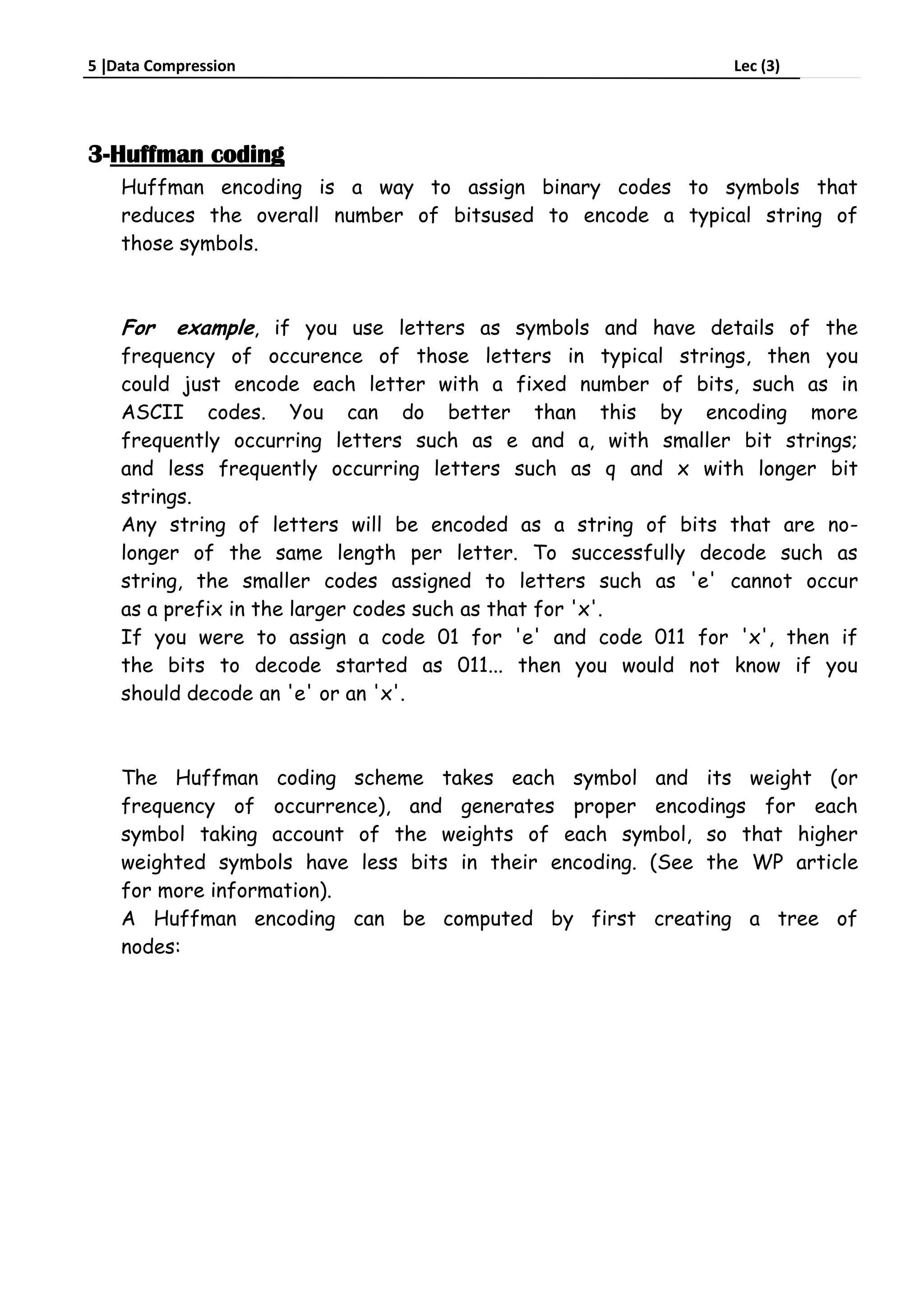
A Huffman encoding can be computed by first creating a tree of
nodes:
6 Data Compression Lec (3)
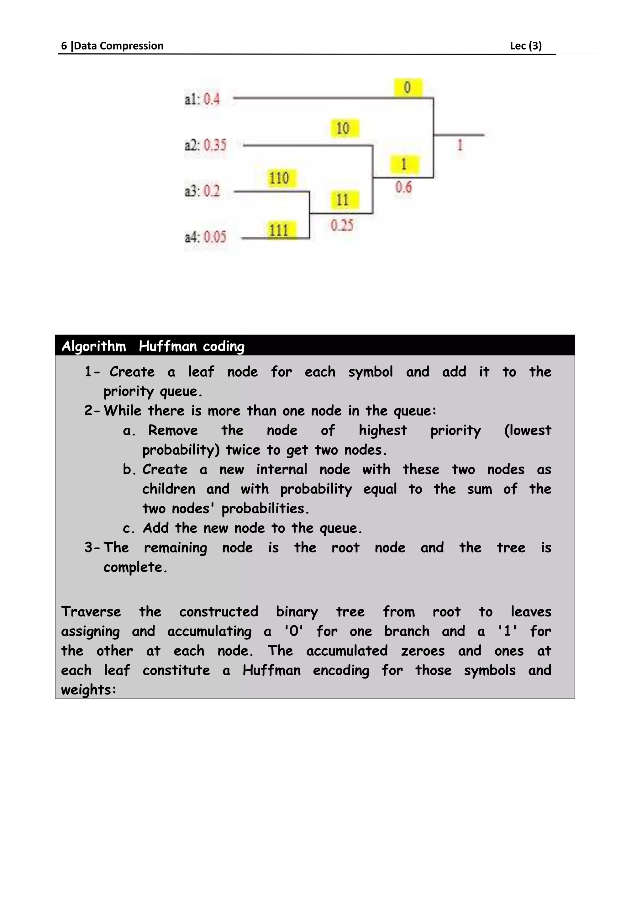
Algorithm Huffman coding
1- Create a leaf node for each symbol and add it to the
priority queue.
2- While there is more than one node in the queue:
a. Remove the node of highest priority (lowest
probability) twice to get two nodes.
b. Create a new internal node with these two nodes as
children and with probability equal to the sum of the
two nodes' probabilities.
c. Add the new node to the queue.
3- The remaining node is the root node and the tree is
complete.
Traverse the constructed binary tree from root to leaves
assigning and accumulating a '0' for one branch and a '1' for
the other at each node. The accumulated zeroes and ones at
each leaf constitute a Huffman encoding for those symbols and
weights:
7 Data Compression Lec (3)
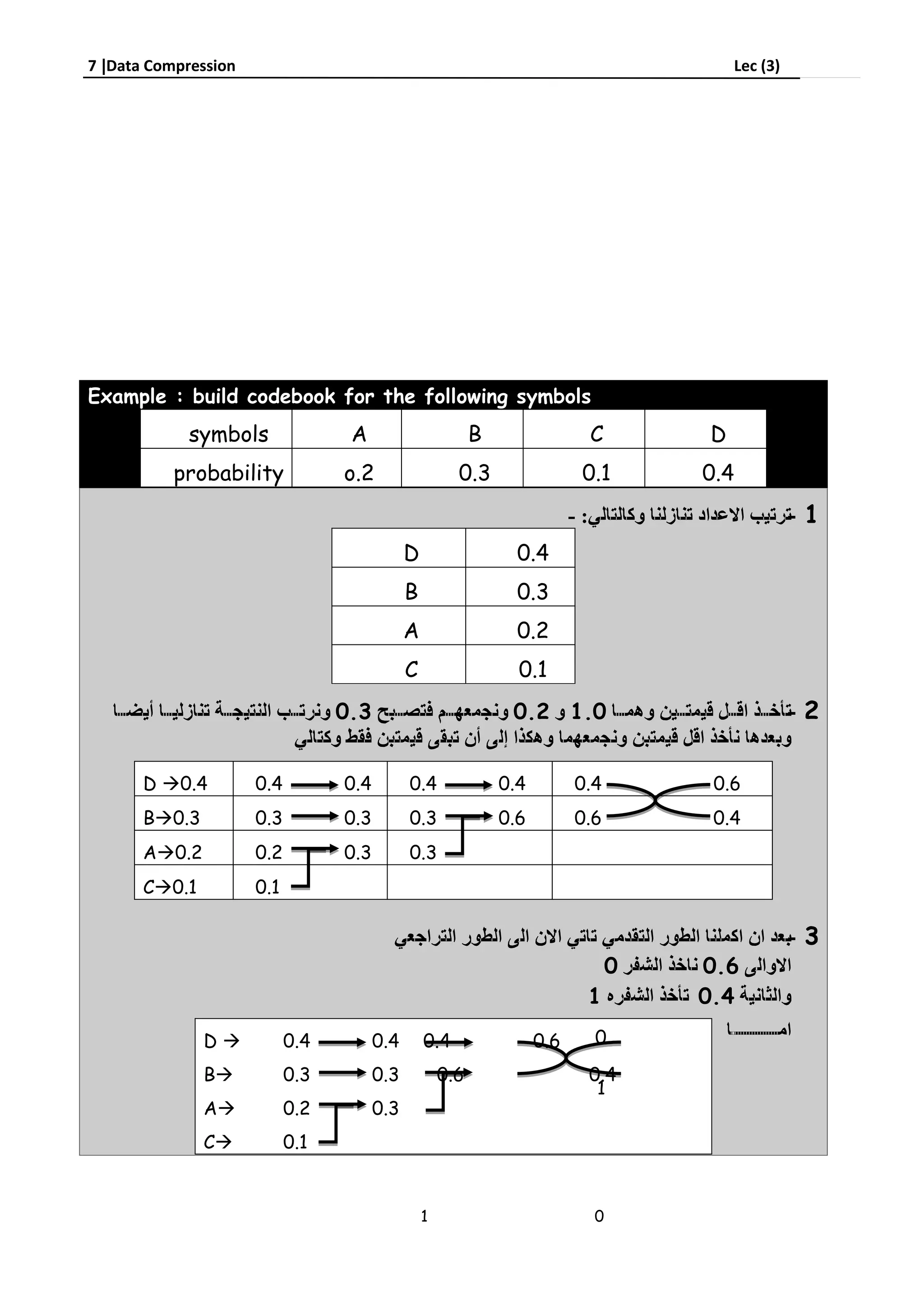
Example : build codebook for the following symbols
symbols A B C D
probability o.2 0.3 0.1 0.4
--
D 0.4
B 0.3
A 0.2
C 0.1
-1.00.20.3
-
0.60
0.41
D 0.4 0.4 0.4 0.4 0.4 0.4 0.6
B0.3 0.3 0.3 0.3 0.6 0.6 0.4
A0.2 0.2 0.3 0.3
C0.1 0.1
D  0.4 0.4 0.4 0.6
B 0.3 0.3 0.6 0.4
A 0.2 0.3
C 0.1
0
1
01
8 Data Compression Lec (3)
01
D  0.4 0.4 0.4 0.6
B 0.3 0.3 0.6 0.4
A 0.2 0.3
C 0.1
D  0.4 0.4 0.4 0.6
B 0.3 0.3 0.6 0.4
A 0.2 0.3
C 0.1
D  0.4 0.4 0.4 0.6
B 0.3 0.3 0.6 0.4
A 0.2 0.3
C 0.1
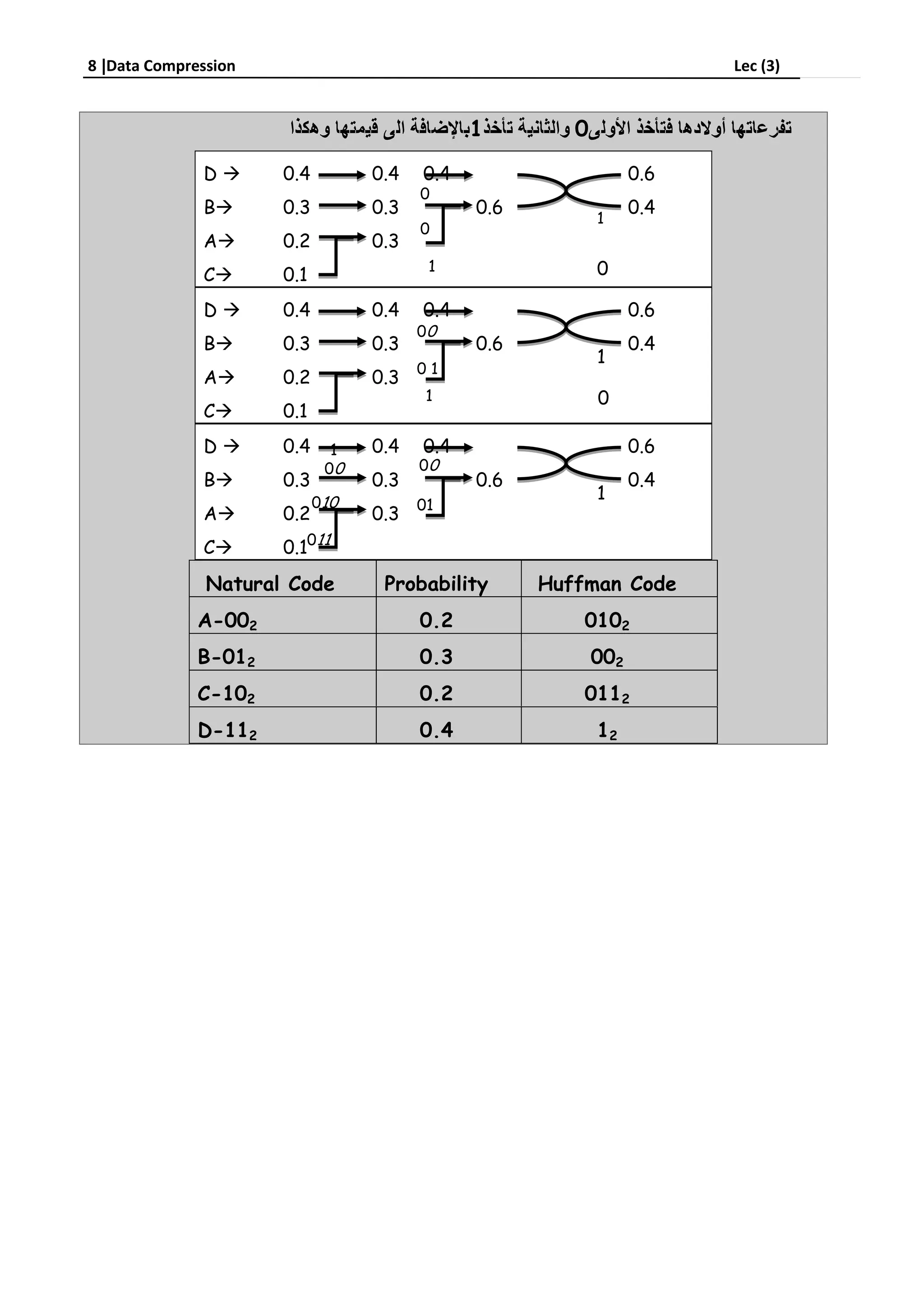
Huffman CodeProbabilityNatural Code
01020.2A-002
0020.3B-012
01120.2C-102
120.4D-112
1
0
0
1
00
0 1
1 0
1
01
01
1
00 00
010
011

Lecft3data

  • 1.
    1 Data CompressionLec (3) - Coding Methods
  • 2.
    2 Data CompressionLec (3) 1-Run-Length Encoding The idea behind this approach to data compression is this: If a data item d occurs nconsecutive times in the input stream, replace the n occurrences with the single pairnd. The n consecutive occurrences of a data item are called a run length of n, and thisapproach to data compression is called run-length encoding or RLE. We apply this ideafirst to text compression and then to image compression.  RLE Text Compression Just replacing 2._all_is_too_well with 2._a2_is_t2_we2 will not work.Even the string 2._a2l_is_t2o_we2l does not solve this problem. One way to solve this problem is to precede each repetition with a special escape character. If we use the character @ as the escape character, then the string 2._a@2l_is_t@2o_we@2l can be decompressed unambiguously. However, this string is longer than the original string, because it replaces two consecutive letters with three characters. We have to adopt the convention that only three or more repetitions of the same character will be replaced with a repetition factor. The main problems with this method are the following: 1. In English text there are not many repetitions. There are many “doubles” but a “triple” is rare. 2. The character “@” may be part of the text in the input stream, in which case a different escape character must be chosen. Sometimes the input stream may contain every possible character in the alphabet.  RLE Image Compression RLE can be used to compress grayscale images. Each run of pixels of the same intensity (gray level) is encoded as a pair (run length, pixel value). The run length usually occupies one byte, allowing for runs of up to 255 pixels. The pixel value occupies several bits, depending on the number of gray levels (typically between 4 and 8 bits).
  • 3.
    3 Data CompressionLec (3) Example 3.1An 8-bit deep grayscale bitmap that starts with 12, 12, 12, 12, 12, 12, 12, 12, 12, 35, 76, 112, 67, 87, 87, 87, 5, 5, 5, 5, 5, 5, 1, . . . is compressed into 9 ,12,35,76,112,67, 3 ,87, 6 ,5,1,. . . , where the bold numbers indicate counts. The problem is to distinguish between a byte containing a grayscale value (such as 12) and one containing a count (such as 9 ). Here are some solutions 1. If the image is limited to just 128 grayscales, we can devote one bit in each byte to indicate whether the byte contains a grayscale value or a count. 2. If the number of grayscales is 256, it can be reduced to 255 with one value reserved as a flag to precede every byte with a count. If the flag is, say, 255, then the sequence above be comes 255, 9, 12, 35, 76, 112, 67, 255, 3, 87, 255, 6, 5, 1, . . . . 3. Again, one bit is devoted to each byte to indicate whether the byte contains a grayscale value or a count. This time, however, these extra bits are accumulated in groups of 8,and each group is written on the output stream preceding (or following) the 8 bytes it “corresponds to.” Example: the sequence 9 ,12,35,76,112,67, 3 ,87, 6 ,5,1,. ... becomes 10000010 ,9,12,35,76,112,67,3,87, 100..... ,6,5,1,. .
  • 4.
    4 Data CompressionLec (3) 2-Move-to-Front Coding The basic idea of this method is to maintain the alphabet A of symbols as a list where frequently occurring symbols are located near the front. A symbol s isencoded as the number of symbols that precede it in this list Example 3.2 Here are example that illustrate the move-to-front idea. The alphabet A=(a, b, c, d, m, n, o, p) The input stream abcddcbamnopponm is encoded as C = (0, 1, 2, 3, 0, 1, 2, 3, 4, 5, 6, 7, 0, 1, 2, 3)
  • 5.
    5 Data CompressionLec (3) 3-Huffman coding Huffman encoding is a way to assign binary codes to symbols that reduces the overall number of bitsused to encode a typical string of those symbols. For example, if you use letters as symbols and have details of the frequency of occurence of those letters in typical strings, then you could just encode each letter with a fixed number of bits, such as in ASCII codes. You can do better than this by encoding more frequently occurring letters such as e and a, with smaller bit strings; and less frequently occurring letters such as q and x with longer bit strings. Any string of letters will be encoded as a string of bits that are no- longer of the same length per letter. To successfully decode such as string, the smaller codes assigned to letters such as 'e' cannot occur as a prefix in the larger codes such as that for 'x'. If you were to assign a code 01 for 'e' and code 011 for 'x', then if the bits to decode started as 011... then you would not know if you should decode an 'e' or an 'x'. The Huffman coding scheme takes each symbol and its weight (or frequency of occurrence), and generates proper encodings for each symbol taking account of the weights of each symbol, so that higher weighted symbols have less bits in their encoding. (See the WP article for more information). A Huffman encoding can be computed by first creating a tree of nodes:
  • 6.
    6 Data CompressionLec (3) Algorithm Huffman coding 1- Create a leaf node for each symbol and add it to the priority queue. 2- While there is more than one node in the queue: a. Remove the node of highest priority (lowest probability) twice to get two nodes. b. Create a new internal node with these two nodes as children and with probability equal to the sum of the two nodes' probabilities. c. Add the new node to the queue. 3- The remaining node is the root node and the tree is complete. Traverse the constructed binary tree from root to leaves assigning and accumulating a '0' for one branch and a '1' for the other at each node. The accumulated zeroes and ones at each leaf constitute a Huffman encoding for those symbols and weights:
  • 7.
    7 Data CompressionLec (3) Example : build codebook for the following symbols symbols A B C D probability o.2 0.3 0.1 0.4 -- D 0.4 B 0.3 A 0.2 C 0.1 -1.00.20.3 - 0.60 0.41 D 0.4 0.4 0.4 0.4 0.4 0.4 0.6 B0.3 0.3 0.3 0.3 0.6 0.6 0.4 A0.2 0.2 0.3 0.3 C0.1 0.1 D  0.4 0.4 0.4 0.6 B 0.3 0.3 0.6 0.4 A 0.2 0.3 C 0.1 0 1 01
  • 8.
    8 Data CompressionLec (3) 01 D  0.4 0.4 0.4 0.6 B 0.3 0.3 0.6 0.4 A 0.2 0.3 C 0.1 D  0.4 0.4 0.4 0.6 B 0.3 0.3 0.6 0.4 A 0.2 0.3 C 0.1 D  0.4 0.4 0.4 0.6 B 0.3 0.3 0.6 0.4 A 0.2 0.3 C 0.1 Huffman CodeProbabilityNatural Code 01020.2A-002 0020.3B-012 01120.2C-102 120.4D-112 1 0 0 1 00 0 1 1 0 1 01 01 1 00 00 010 011