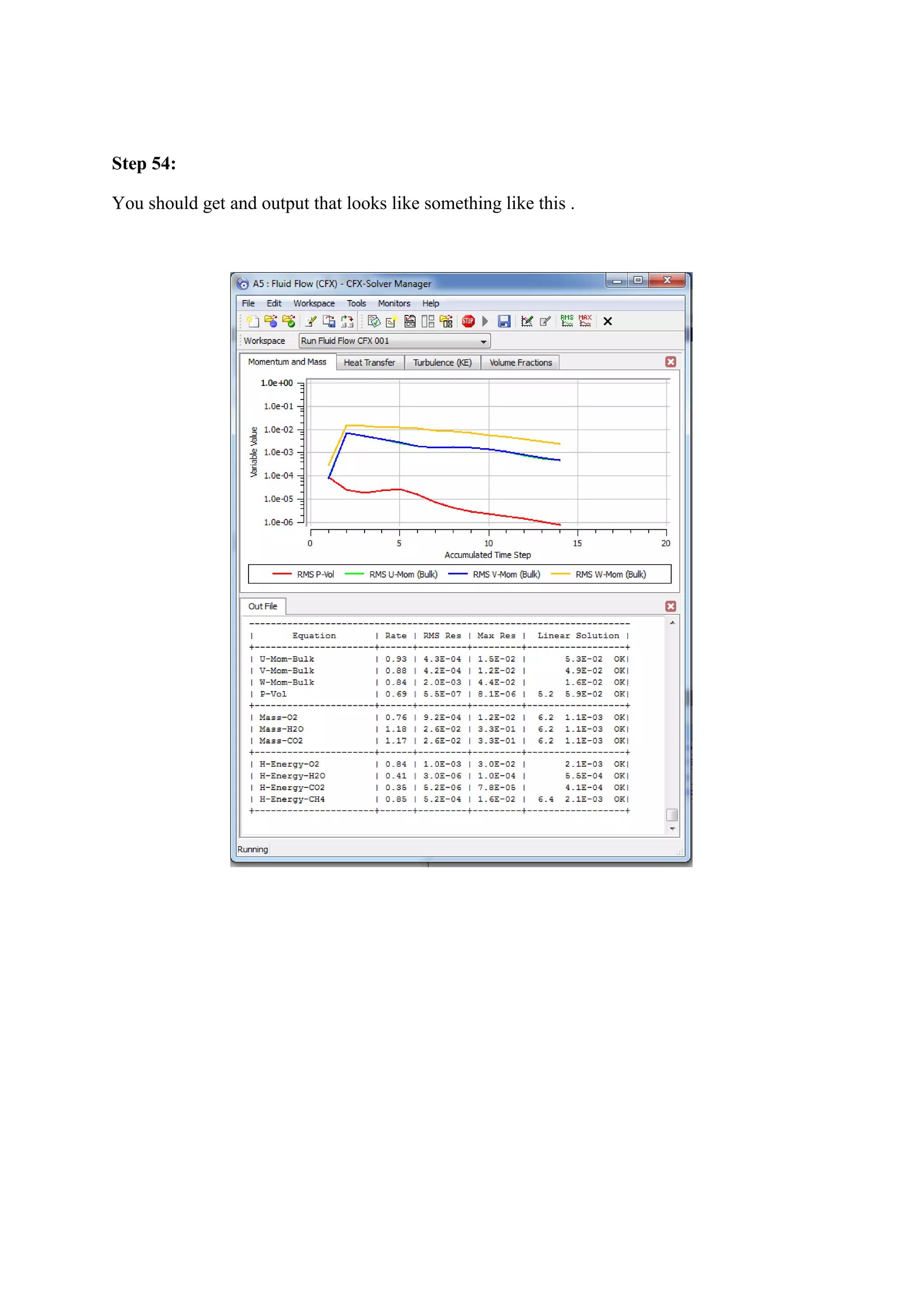
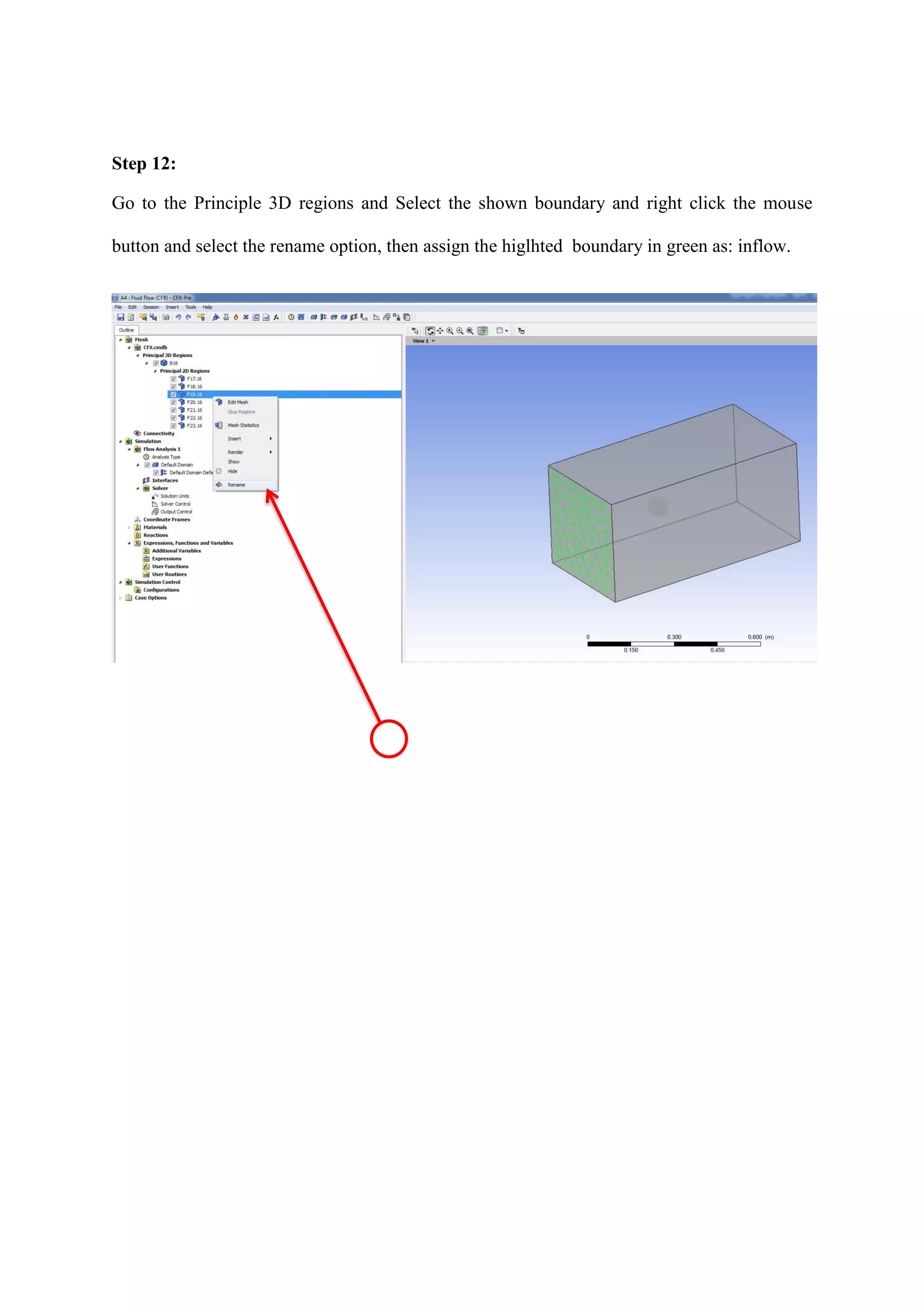
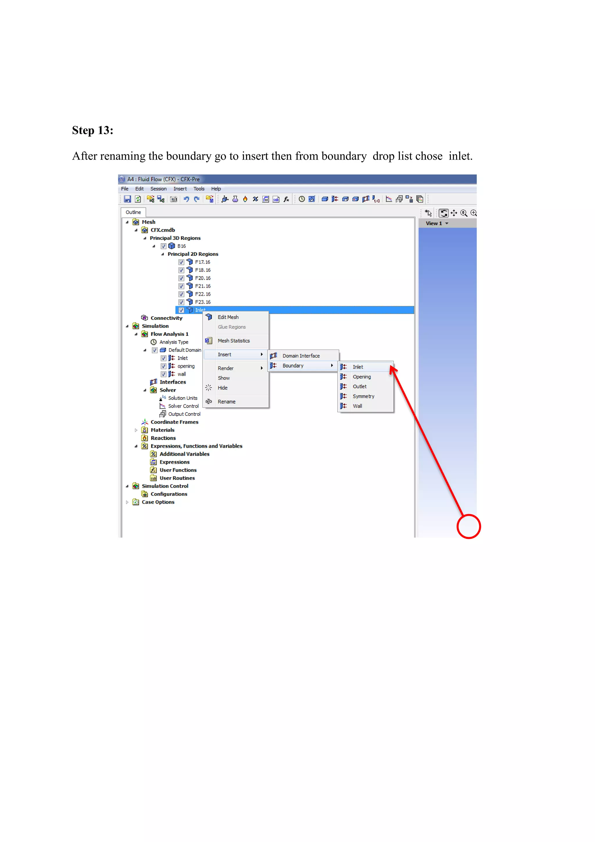
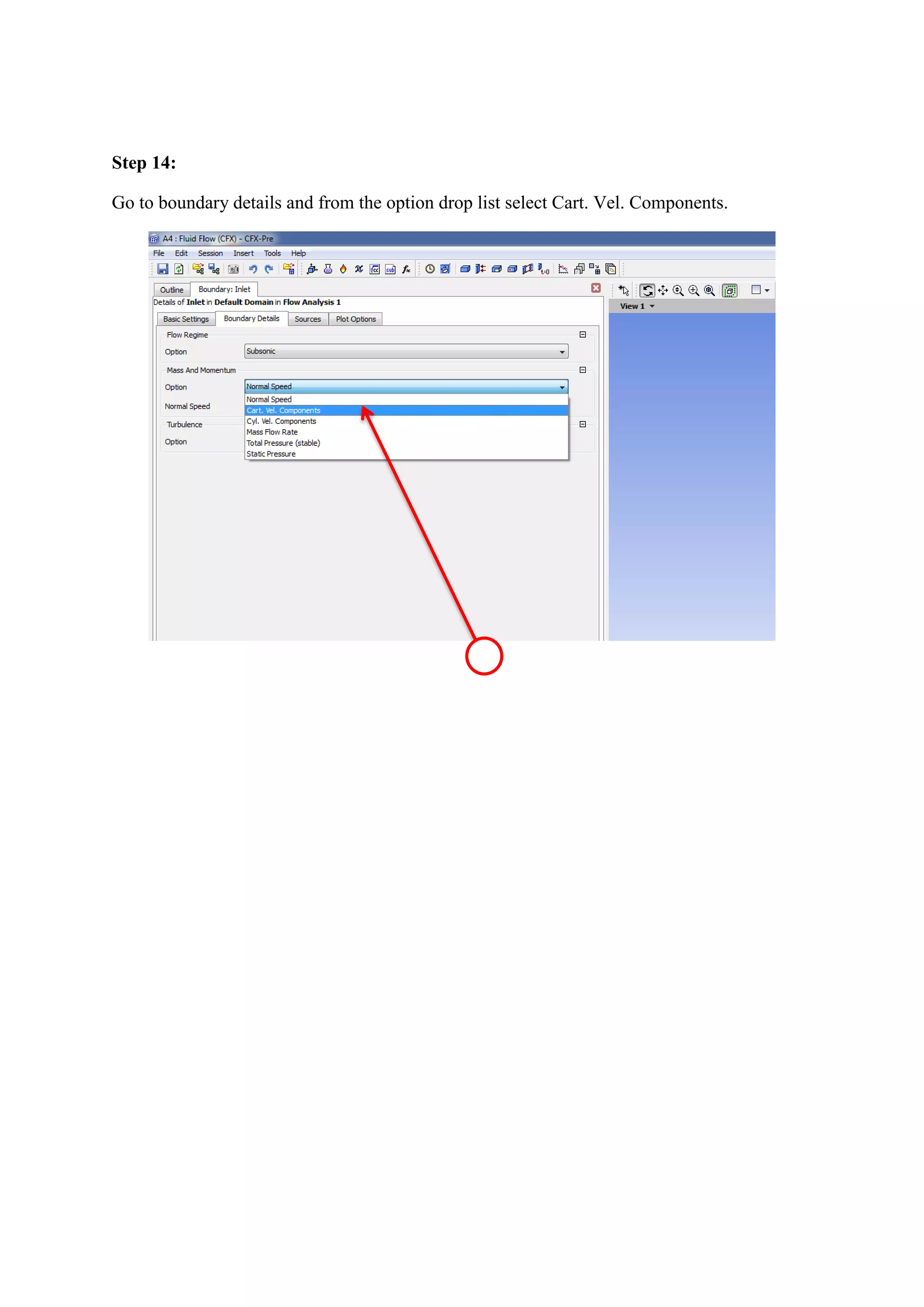
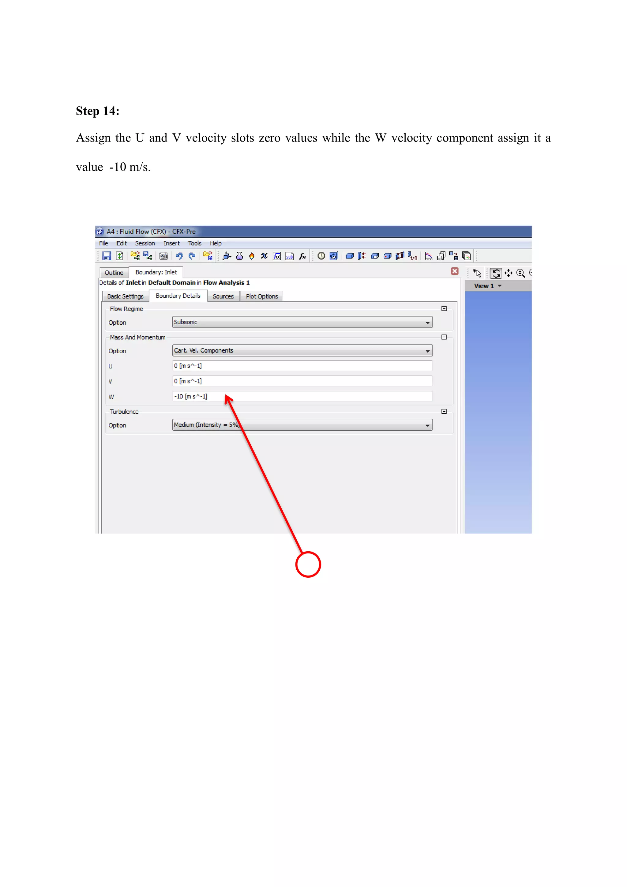
SlideShare a Scribd company logo
Methane Combustion Modelling Tutorial using ANSYS CFX 
First Edition 
By Ahmed Al Makkky
@Ahmed Al Makky 2012 
All rights reserved. No part of this publication may be reproduced, stored in a retrieval system or transmitted in any form or by any means, electronic, mechanical or photo-copying, recording, or otherwise without the prior permission of the publisher.
Methane Combustion modelling using ANSYS CFX 
Introduction 
The tutorial was written in a rush so it has spelling mistakes never go the time to correct them, feedback would much appreciated to improve the tutorials. A mesh file is provided with this tutorial in order to focus on the combustion simulation. Combustion is encountered in most engineering applications. Ranging from boilers to gas turbines to internal combustion engines…..etc. This tutorial guides the researcher through a step by step process to get a simple combustion done. From this tutorial the user will be able to get the general required guideline to conduct a combustion simulation. This tutorial might have some inaccurate input values but no need to worry about that at the moment because at this stage it is essential to get an initial simulation run then we can proceed in making more accurate input value selection. The mesh is made with a ball forming an obstacle in the flow. The main intention of having that ball is to form a circulation filed after it and also to form a source of ignition to the mixture. This is done through assigning the ball surface a heat source term.
Step 1: 
The first step is to double click the Fluid Flow (CFX) icon, then the next step is to double click on the geometry icon the has beside it the question blue mark.
Step 2: 
Under file drop down list select Import External Geometry file. You need to remmber that the file is provided with this tutorial. This tutorial skips the modelling part of the project so there is no need to use DesignModeller. If you do not have a ready mesh then it is essential to model your mesh using DesignModeller.
Step 3: 
A window will open up select the file named Ball.x_t. and then press open.
Step 4: 
Go back to the main list and check that the green tick sogn is visible beside the geometry icon and then double click the Mesh icon.
Step 5: 
Right Click on method then select insert and then from insert select method.
Step 6: 
The next step is by clicking on the mesh box which results in it turning into green then pressing the Apply icon in the geometry section.
Step 8: 
Click on the update to command the Mehser to start generating the mesh.
Step 9: 
By looking where the arrow is pointing you can see the mesh generation process is being done. Just to note that if the meshing process takes more than 5 minutes than most probably no mesh would be generated.
Step 10: 
Click the left button on the mouse on the mesh icon to clarfiy that the mesh has been generated.
Step 11: 
Check that the green tick is beside the mesh sign then double click the setup icon.
Step 12: 
Go to the Principle 3D regions and Select the shown boundary and right click the mouse button and select the rename option, then assign the higlhted boundary in green as: inflow.
Step 13: 
After renaming the boundary go to insert then from boundary drop list chose inlet.
Step 14: 
Go to boundary details and from the option drop list select Cart. Vel. Components.
Step 14: 
Assign the U and V velocity slots zero values while the W velocity component assign it a value -10 m/s.
Step 13: 
Choose the ball surface and assign it a wall condition and press Ok. At a later stage we will assign this wall a heat source which would perform the role of flame holder.
Step 14: 
Select all the 5 boundaries using the control button and the mouse cursor to select the required boundary.
Step 15: 
Type in the pressure value of 101325 Pa which represnts atmospheric conditions. Then press Ok.
Step 16: 
Check that there is a green tick in the setup section then double click the solution icon.
Step 17: 
If you have a single core machine then keep the selection as serial while for more extensive calculations then HP MPI Local Parallel is advisable.
Step 18: 
The first step is click on the plus icon till the number of partitions gets to four; this would help to conduct a parallel calculation on the lab quad core desktop. A note to the user that he has to check what kind of processor his desktop is.
Step 19: 
By running a simulation the user can initialy clarfiy that the domain is applicapble to run a combustion simulation.
Step 20: 
The visulization part comes here, it starts by double clicking on the results icon.
Step 21: 
By using the vector representation to visualize the flow pattern the user can clarify that his input parameters are correct.
Step 20: 
Then comes selecting the required domain for the vector field which is in the studied case the default domain and then press Ok.
Step 22: 
By looking closely at the vector tip direction the user can clarfiy that the flow field is. Mimicing the case he wants.
Step 23: 
The next step is to go back to the fluid flow (CFX) and double click on the setup icon. This is where we start working on the combustion side of things. 
Note : Regarding important values for the combustion simulation the researcher can extract lots of the needed data from the following reference: 
http://www.amazon.co.uk/An-Introduction-Combustion-Concepts- Applications/dp/0071260722/ref=cm_cr-mr-title 
This handbook is also rich with important data to: 
http://www.amazon.co.uk/Combustion-Engineering-Computational-Mechanics- Analysis/dp/0849320712/ref=cm_cr-mr-title 
If you want to learn more about flamelets and computational combustion simulation: 
http://www.amazon.co.uk/Theoretical-Numerical-Combustion-2- E/dp/1930217102/ref=cm_cr-mr-title
Step 24: 
By right clicking on the Default Domain icon what comes next is selecting the edit option.
Step 25: 
Under the basic setting you will see that by defual Fluid 1 is assigned by the software which represnts Air at a temperaure of 25. We are not concerned with air for our studied case for combustion case of Methane which will be our studied case we will need four species to be taken into account based on the following equation: ( ) ( ) → ( ) ( ) 
By clicking on the x red button the Fluid 1 is deleted from the list and we can proceed to add the gas species we want to add.
Step 26: 
To add the required species click on the icon that has a document with a yellow star to add a new species. You can start with which ever species you like. I started with carbon dioixde then water vapour then oxygen and finally methane. Remmber that we have just assigned the names of the species, the next step is to asign the thermodynamic properties to the species we have just named.
Step 27: 
To acsess the thermodynamic properties of the different specise we have to call the library which is provided with the software.
Step 28: 
When you open the library a new window is visible. Go to the gas phase combustion section and select the four required species which we named earlier and then press Ok. What you will notice that after pressing Ok the four species have been transferred to the material window. 
:
Step 29: 
The thermodynamic species have been specfied the next step is to link thermodynamic quantities with our named species.
Step 30: 
What comes next is we need to select the Fluid model the importance of this that by selecting the Thermal Energy option from the drop down list we can assign the tempeature heat source term to the sphere surface which would perform the ignition source to the chemical reaction.
Step 31: 
The next step is click the tick boxes for a Homogeneous Model for the Multiphase part and for the Homogeneous Model for the Heat Transfer part.
Step 32: 
The next step is to define the occuring reaction in the flow this is done through right clicking on the Reactions folder in the Outline section and then from the insert drop down list select Reaction.
Step 33: 
By default the reactants is specfied as Air Ideal Gas, while for our case are the two species in the red color shown in the following equation: ( ) ( ) → ( ) ( )
Step 34: 
So we add the two species by pressing on the squred box and from the drop list selecting Methane and Oxygen.
Step 34: 
It is visible from the material list that Methane and oxygen have been added. ( ) ( ) → ( ) ( ) 
First of all we select methane in the Child Materials list. The stoichiometric coefficient is shown in green and is taken having the value of one. The reaction order therfore as a consequance the reaction order is taken as 1.
Step 35: 
We select oxygen from the Child Materials list. ( ) ( ) → ( ) ( ) 
The stoichiometric Coefficient is taken 2 for oxygen represented in green in the previous equation. Therefore the reaction order is taken as 2.
Step 34: 
Next step is to select carbon dioxide and water vapour as products of combustion as seen in the red coloured species in the equation below: ( ) ( ) → ( ) ( ) 
We can see that the default species is chosen as Air ideal gas, by pressing on the materials list box we can access the library of species, under the gas phase combustion list select C
Step 35: 
After pressing ok we find that the two species have been added under the Child Materials list. We select carbon dioxide in the Child Materials list. ( ) ( ) → ( ) ( ) 
From the previous equation we can see that the stoichiometric Coefficient is 1. Therefore the reaction order is 1.
Step 36: 
The next step in the products section is to select water vapour shown in red in the equation below: ( ) ( ) → ( ) ( ) 
By selecting the water vapour species in the Child Materials list, we take the Stoichiometric coefficient as 2 which is seen in green in the equation above.
Step 37: 
The following step is to work on the Reaction Rates section, the reaction rate equation is shown below: ( )[ ] [ ] 
what is of our intrest is the raction rate coefficient ( ) which is also known as the arrahnuies equatiion: ( ) 
What will be required by us is to find in litrature the following values starting with the pre exponential factor: 
The activation temperature in the exponential part is: 
The activation energy: 
By substituting all the found values in the required cells we can finally press apply and Ok.
Step 38: 
In this section we start applying the volume fractions at the boundary conditions. We start with the inlet section where we select it under the Default Domain in the Outline Section. Then Edit is selected.
Step 39: 
Under the fluid values section we will consider that methane has a volume fraction of 0.5. 
Step 40: 
Due to that we consider no combustion occuring previously we can take carbon dixode volume fraction as 0.
Step 41: 
Due to that we consider dry air is flowing into the combustor we can take the water vapour volume fraction as 0. 
Step 42: 
Finaly a combustion process needs an oxidzer therfore we take the volume fraction of oxygen as 0.5.
Step 43: 
The next step under boundary details we select an input velocity of -10 m/s. The reason for a minus sign is due to the direction of the flow in the mesh is in the opposite direction of default coordinate system in Fluid Flow(CFX). While the rest of the velocities are takenas zero. Finaly the ambient temperature is taken as 300K.
Step 44: 
The next step is to assign the opening section the species volume fractions. By selecting the openning boundary and then selecting edit.
Step 45: 
By going to the fluid values section and selecting the required species volume fractions. The opening volume fraction for methane is taken as 0.1.
Step 46: 
The opening volume fraction for Carbon dixode is taken as 0.1
Step 47: 
The opening volume fraction for water vapour is taken as 0.4. 
Step 48: 
The opening volume fraction for oxygen is taken as 0.1.
Step 49: 
The next step is to go to the boundary details and choose the Relative Pressure as 101325 Pa.
Step 50: 
In this step we edit the wall boundary condition for the located sphere inside the meshed domain, so by right clicking on the wall icon and then selecting the edit option. 
Step 51: 
Then in this step we go to the Boundary Details and apply the Fixed Temperature value of 2000K and then press apply and Ok.
Step 52: 
Congratulations the setting up process is finished go back to the project schematic view and double click on solution.
Step 53: 
You can use the serial mode to run your calculation but I would prefer to make use of the quad core machine I am working on.
Step 54: 
You should get and output that looks like something like this .

More Related Content

What's hot

Heat transfer
Heat transferHeat transfer
Heat transfer
Home
 
Piston
PistonPiston
Piston
jzamora3521
 
sectional views
sectional viewssectional views
sectional views
vikash singh
 
Chap09 ht 3e natural convection
Chap09 ht 3e natural convectionChap09 ht 3e natural convection
Chap09 ht 3e natural convection
Bening Kambuna
 
Numerical methods for 2 d heat transfer
Numerical methods for 2 d heat transferNumerical methods for 2 d heat transfer
Numerical methods for 2 d heat transfer
Arun Sarasan
 
CATIA V5 Lectures.ppt
CATIA V5 Lectures.pptCATIA V5 Lectures.ppt
CATIA V5 Lectures.ppt
PoojaTripathi92
 
Expressions for shape functions of linear element
Expressions for shape functions of linear element Expressions for shape functions of linear element
Expressions for shape functions of linear element
Sharath Kumar
 
Chapter 7 EXTERNAL FORCED CONVECTION
Chapter 7EXTERNAL FORCED CONVECTIONChapter 7EXTERNAL FORCED CONVECTION
Chapter 7 EXTERNAL FORCED CONVECTION
Abdul Moiz Dota
 
Steady- state-heat-transfer-in-multiple-dimensions
Steady- state-heat-transfer-in-multiple-dimensionsSteady- state-heat-transfer-in-multiple-dimensions
Steady- state-heat-transfer-in-multiple-dimensions
tmuliya
 
Dual cycle
Dual cycleDual cycle
Dual cycle
Harshal Bhatt
 
One dim, steady-state, heat conduction_with_heat_generation
One dim, steady-state, heat conduction_with_heat_generationOne dim, steady-state, heat conduction_with_heat_generation
One dim, steady-state, heat conduction_with_heat_generation
tmuliya
 
APPLIED THERMODYNAMICS 18ME42 Module 01 question no 2a &2b
APPLIED THERMODYNAMICS 18ME42 Module 01 question no 2a &2bAPPLIED THERMODYNAMICS 18ME42 Module 01 question no 2a &2b
APPLIED THERMODYNAMICS 18ME42 Module 01 question no 2a &2b
THANMAY JS
 
Heat 4e chap08_lecture
Heat 4e chap08_lectureHeat 4e chap08_lecture
Heat 4e chap08_lecture
Abdul Moiz Dota
 
Introduction to Engineering Graphics
Introduction to Engineering Graphics Introduction to Engineering Graphics
Introduction to Engineering Graphics
Nitin Shekapure
 
Applied thermodynamics(lecture 1)
Applied thermodynamics(lecture 1)Applied thermodynamics(lecture 1)
Applied thermodynamics(lecture 1)
TAUSIQUE SHEIKH
 
Properties of pure substances
Properties of pure substancesProperties of pure substances
Properties of pure substances
HarishDAV
 
Revision on thermodynamics
Revision on thermodynamicsRevision on thermodynamics
Revision on thermodynamics
cairo university
 
Knocking & detonation
Knocking & detonationKnocking & detonation
Knocking & detonation
Qabool Ahmed Memon
 
Chap 35 ppt
Chap 35 pptChap 35 ppt
Chap 35 ppt
Mulugeta Wotango
 
Lecture # 5 cost estimation i
Lecture # 5 cost estimation iLecture # 5 cost estimation i
Lecture # 5 cost estimation i
Bich Lien Pham
 

What's hot (20)

Heat transfer
Heat transferHeat transfer
Heat transfer
 
Piston
PistonPiston
Piston
 
sectional views
sectional viewssectional views
sectional views
 
Chap09 ht 3e natural convection
Chap09 ht 3e natural convectionChap09 ht 3e natural convection
Chap09 ht 3e natural convection
 
Numerical methods for 2 d heat transfer
Numerical methods for 2 d heat transferNumerical methods for 2 d heat transfer
Numerical methods for 2 d heat transfer
 
CATIA V5 Lectures.ppt
CATIA V5 Lectures.pptCATIA V5 Lectures.ppt
CATIA V5 Lectures.ppt
 
Expressions for shape functions of linear element
Expressions for shape functions of linear element Expressions for shape functions of linear element
Expressions for shape functions of linear element
 
Chapter 7 EXTERNAL FORCED CONVECTION
Chapter 7EXTERNAL FORCED CONVECTIONChapter 7EXTERNAL FORCED CONVECTION
Chapter 7 EXTERNAL FORCED CONVECTION
 
Steady- state-heat-transfer-in-multiple-dimensions
Steady- state-heat-transfer-in-multiple-dimensionsSteady- state-heat-transfer-in-multiple-dimensions
Steady- state-heat-transfer-in-multiple-dimensions
 
Dual cycle
Dual cycleDual cycle
Dual cycle
 
One dim, steady-state, heat conduction_with_heat_generation
One dim, steady-state, heat conduction_with_heat_generationOne dim, steady-state, heat conduction_with_heat_generation
One dim, steady-state, heat conduction_with_heat_generation
 
APPLIED THERMODYNAMICS 18ME42 Module 01 question no 2a &2b
APPLIED THERMODYNAMICS 18ME42 Module 01 question no 2a &2bAPPLIED THERMODYNAMICS 18ME42 Module 01 question no 2a &2b
APPLIED THERMODYNAMICS 18ME42 Module 01 question no 2a &2b
 
Heat 4e chap08_lecture
Heat 4e chap08_lectureHeat 4e chap08_lecture
Heat 4e chap08_lecture
 
Introduction to Engineering Graphics
Introduction to Engineering Graphics Introduction to Engineering Graphics
Introduction to Engineering Graphics
 
Applied thermodynamics(lecture 1)
Applied thermodynamics(lecture 1)Applied thermodynamics(lecture 1)
Applied thermodynamics(lecture 1)
 
Properties of pure substances
Properties of pure substancesProperties of pure substances
Properties of pure substances
 
Revision on thermodynamics
Revision on thermodynamicsRevision on thermodynamics
Revision on thermodynamics
 
Knocking & detonation
Knocking & detonationKnocking & detonation
Knocking & detonation
 
Chap 35 ppt
Chap 35 pptChap 35 ppt
Chap 35 ppt
 
Lecture # 5 cost estimation i
Lecture # 5 cost estimation iLecture # 5 cost estimation i
Lecture # 5 cost estimation i
 

Viewers also liked

Artificial reefs
Artificial reefsArtificial reefs
Artificial reefs
Yasser Ahmed
 
Cfx12 04 solver
Cfx12 04 solverCfx12 04 solver
Cfx12 04 solver
Arvind Srinivasan
 
Cfx12 08 transient
Cfx12 08 transientCfx12 08 transient
Cfx12 08 transient
Marcushuynh66
 
Cfx12 11 cel
Cfx12 11 celCfx12 11 cel
Cfx12 11 cel
Marcushuynh66
 
Cfx12 13 ccl_out_file
Cfx12 13 ccl_out_fileCfx12 13 ccl_out_file
Cfx12 13 ccl_out_file
Marcushuynh66
 
Cfx12 07 physics2
Cfx12 07 physics2Cfx12 07 physics2
Cfx12 07 physics2
Marcushuynh66
 
Final Exam Ansys CFX - Stephen White
Final Exam Ansys CFX - Stephen WhiteFinal Exam Ansys CFX - Stephen White
Final Exam Ansys CFX - Stephen White
Stephen White
 
Cfx12 11 cel
Cfx12 11 celCfx12 11 cel
Cfx12 11 cel
al11429964
 
Advanced Simulations of Hypertrophic Obstructive Cardiomyopathy in Human Hear...
Advanced Simulations of Hypertrophic Obstructive Cardiomyopathy in Human Hear...Advanced Simulations of Hypertrophic Obstructive Cardiomyopathy in Human Hear...
Advanced Simulations of Hypertrophic Obstructive Cardiomyopathy in Human Hear...
Can Ozcan
 
Cfx12 06 review_day1
Cfx12 06 review_day1Cfx12 06 review_day1
Cfx12 06 review_day1
Marcushuynh66
 
Cfx12 12 moving_zones
Cfx12 12 moving_zonesCfx12 12 moving_zones
Cfx12 12 moving_zones
Marcushuynh66
 
CFX Certificate
CFX CertificateCFX Certificate
CFX Certificate
Mehdi Ghobadi , PhD., MBA
 
Cfx12 00 toc_welcome
Cfx12 00 toc_welcomeCfx12 00 toc_welcome
Cfx12 00 toc_welcome
Marcushuynh66
 
The Return on Investment of Computational Fluid Dynamics
The Return on Investment of Computational Fluid DynamicsThe Return on Investment of Computational Fluid Dynamics
The Return on Investment of Computational Fluid Dynamics
Ansys
 
CFX:Mixing T-Junction
CFX:Mixing T-JunctionCFX:Mixing T-Junction
CFX:Mixing T-Junction
Preeda Prakotmak
 
Cfx12 02 intro_cfx
Cfx12 02 intro_cfxCfx12 02 intro_cfx
Cfx12 02 intro_cfx
Marcushuynh66
 
Cfx12 09 turbulence
Cfx12 09 turbulenceCfx12 09 turbulence
Cfx12 09 turbulence
Marcushuynh66
 
Simulations of Hypertrophic Obstructive Cardiomyopathy (HOCM) in a Human Hear...
Simulations of Hypertrophic Obstructive Cardiomyopathy (HOCM) in a Human Hear...Simulations of Hypertrophic Obstructive Cardiomyopathy (HOCM) in a Human Hear...
Simulations of Hypertrophic Obstructive Cardiomyopathy (HOCM) in a Human Hear...
Can Ozcan
 
Cfx12 10 heat_transfer
Cfx12 10 heat_transferCfx12 10 heat_transfer
Cfx12 10 heat_transfer
Marcushuynh66
 
Cfx12 11 cel_printing
Cfx12 11 cel_printingCfx12 11 cel_printing
Cfx12 11 cel_printing
Marcushuynh66
 

Viewers also liked (20)

Artificial reefs
Artificial reefsArtificial reefs
Artificial reefs
 
Cfx12 04 solver
Cfx12 04 solverCfx12 04 solver
Cfx12 04 solver
 
Cfx12 08 transient
Cfx12 08 transientCfx12 08 transient
Cfx12 08 transient
 
Cfx12 11 cel
Cfx12 11 celCfx12 11 cel
Cfx12 11 cel
 
Cfx12 13 ccl_out_file
Cfx12 13 ccl_out_fileCfx12 13 ccl_out_file
Cfx12 13 ccl_out_file
 
Cfx12 07 physics2
Cfx12 07 physics2Cfx12 07 physics2
Cfx12 07 physics2
 
Final Exam Ansys CFX - Stephen White
Final Exam Ansys CFX - Stephen WhiteFinal Exam Ansys CFX - Stephen White
Final Exam Ansys CFX - Stephen White
 
Cfx12 11 cel
Cfx12 11 celCfx12 11 cel
Cfx12 11 cel
 
Advanced Simulations of Hypertrophic Obstructive Cardiomyopathy in Human Hear...
Advanced Simulations of Hypertrophic Obstructive Cardiomyopathy in Human Hear...Advanced Simulations of Hypertrophic Obstructive Cardiomyopathy in Human Hear...
Advanced Simulations of Hypertrophic Obstructive Cardiomyopathy in Human Hear...
 
Cfx12 06 review_day1
Cfx12 06 review_day1Cfx12 06 review_day1
Cfx12 06 review_day1
 
Cfx12 12 moving_zones
Cfx12 12 moving_zonesCfx12 12 moving_zones
Cfx12 12 moving_zones
 
CFX Certificate
CFX CertificateCFX Certificate
CFX Certificate
 
Cfx12 00 toc_welcome
Cfx12 00 toc_welcomeCfx12 00 toc_welcome
Cfx12 00 toc_welcome
 
The Return on Investment of Computational Fluid Dynamics
The Return on Investment of Computational Fluid DynamicsThe Return on Investment of Computational Fluid Dynamics
The Return on Investment of Computational Fluid Dynamics
 
CFX:Mixing T-Junction
CFX:Mixing T-JunctionCFX:Mixing T-Junction
CFX:Mixing T-Junction
 
Cfx12 02 intro_cfx
Cfx12 02 intro_cfxCfx12 02 intro_cfx
Cfx12 02 intro_cfx
 
Cfx12 09 turbulence
Cfx12 09 turbulenceCfx12 09 turbulence
Cfx12 09 turbulence
 
Simulations of Hypertrophic Obstructive Cardiomyopathy (HOCM) in a Human Hear...
Simulations of Hypertrophic Obstructive Cardiomyopathy (HOCM) in a Human Hear...Simulations of Hypertrophic Obstructive Cardiomyopathy (HOCM) in a Human Hear...
Simulations of Hypertrophic Obstructive Cardiomyopathy (HOCM) in a Human Hear...
 
Cfx12 10 heat_transfer
Cfx12 10 heat_transferCfx12 10 heat_transfer
Cfx12 10 heat_transfer
 
Cfx12 11 cel_printing
Cfx12 11 cel_printingCfx12 11 cel_printing
Cfx12 11 cel_printing
 

Similar to Combustion modelling using_ansys_cfx

PresentationCrystalReport.ppt
PresentationCrystalReport.pptPresentationCrystalReport.ppt
PresentationCrystalReport.ppt
DIGVIJAYPATIL831104
 
PresentationCrystaljoiuouoouououoooiuiouiououoioiuoiuouo
PresentationCrystaljoiuouoouououoooiuiouiououoioiuoiuouoPresentationCrystaljoiuouoouououoooiuiouiououoioiuoiuouo
PresentationCrystaljoiuouoouououoooiuiouiououoioiuoiuouo
hrhedgewarhospital
 
GIS AUTOMATION
GIS AUTOMATIONGIS AUTOMATION
GIS AUTOMATION
William Francis
 
FINE FIRE BIM SOFTWARE - Step by step tutorial guide
FINE FIRE BIM SOFTWARE - Step by step tutorial guideFINE FIRE BIM SOFTWARE - Step by step tutorial guide
FINE FIRE BIM SOFTWARE - Step by step tutorial guide
Isidoros Siderakis
 
Workshop16 heat-pipejoint
Workshop16 heat-pipejointWorkshop16 heat-pipejoint
Workshop16 heat-pipejoint
mmd110
 
Hysys tutorial
Hysys tutorialHysys tutorial
Hysys tutorial
Bijol Luis
 
Thermal Analysis in Hypermesh (Conduction, Convention and Thermal Expansion)
Thermal Analysis in Hypermesh (Conduction, Convention and Thermal Expansion)Thermal Analysis in Hypermesh (Conduction, Convention and Thermal Expansion)
Thermal Analysis in Hypermesh (Conduction, Convention and Thermal Expansion)
Akshay Mistri
 
Tutorials2
Tutorials2Tutorials2
Tutorials2
raja umair
 
Chapter 08
Chapter 08Chapter 08
Chapter 08
llmeade
 
Sliding door
Sliding doorSliding door
Sliding door
Mohamed Al-Attar
 
COSC 1436 Project Page 1 Pre Project Example Secti.docx
COSC 1436 Project Page 1  Pre Project Example Secti.docxCOSC 1436 Project Page 1  Pre Project Example Secti.docx
COSC 1436 Project Page 1 Pre Project Example Secti.docx
faithxdunce63732
 
Dipole
DipoleDipole
The Role of CFD in Real Life Designs
The Role of CFD in Real Life DesignsThe Role of CFD in Real Life Designs
The Role of CFD in Real Life Designs
SOLIDWORKS
 
Magazine awr-ims-3
Magazine awr-ims-3Magazine awr-ims-3
Magazine awr-ims-3
Sam Sambala
 
ECRIN SAPHIR TUTORIAL Dr. P. Ghahri Prepared by.docx
ECRIN SAPHIR TUTORIAL Dr. P. Ghahri Prepared by.docxECRIN SAPHIR TUTORIAL Dr. P. Ghahri Prepared by.docx
ECRIN SAPHIR TUTORIAL Dr. P. Ghahri Prepared by.docx
tidwellveronique
 
Episode 52 : Flow sheeting Case Study
Episode 52 :  Flow sheeting Case StudyEpisode 52 :  Flow sheeting Case Study
Episode 52 : Flow sheeting Case Study
SAJJAD KHUDHUR ABBAS
 
Solid Modeling Assignment EGR 201-100 Spring 2018 .docx
Solid Modeling Assignment EGR 201-100 Spring 2018 .docxSolid Modeling Assignment EGR 201-100 Spring 2018 .docx
Solid Modeling Assignment EGR 201-100 Spring 2018 .docx
whitneyleman54422
 
Rhino to Ecotect
Rhino to EcotectRhino to Ecotect
Rhino to Ecotect
NYCCTfab
 
Executing tools-in-modelbuilder-tutorial
Executing tools-in-modelbuilder-tutorialExecuting tools-in-modelbuilder-tutorial
Executing tools-in-modelbuilder-tutorial
askar_gila
 
Mentor manual
Mentor manualMentor manual
Mentor manual
basavaraju ramaduragam
 

Similar to Combustion modelling using_ansys_cfx (20)

PresentationCrystalReport.ppt
PresentationCrystalReport.pptPresentationCrystalReport.ppt
PresentationCrystalReport.ppt
 
PresentationCrystaljoiuouoouououoooiuiouiououoioiuoiuouo
PresentationCrystaljoiuouoouououoooiuiouiououoioiuoiuouoPresentationCrystaljoiuouoouououoooiuiouiououoioiuoiuouo
PresentationCrystaljoiuouoouououoooiuiouiououoioiuoiuouo
 
GIS AUTOMATION
GIS AUTOMATIONGIS AUTOMATION
GIS AUTOMATION
 
FINE FIRE BIM SOFTWARE - Step by step tutorial guide
FINE FIRE BIM SOFTWARE - Step by step tutorial guideFINE FIRE BIM SOFTWARE - Step by step tutorial guide
FINE FIRE BIM SOFTWARE - Step by step tutorial guide
 
Workshop16 heat-pipejoint
Workshop16 heat-pipejointWorkshop16 heat-pipejoint
Workshop16 heat-pipejoint
 
Hysys tutorial
Hysys tutorialHysys tutorial
Hysys tutorial
 
Thermal Analysis in Hypermesh (Conduction, Convention and Thermal Expansion)
Thermal Analysis in Hypermesh (Conduction, Convention and Thermal Expansion)Thermal Analysis in Hypermesh (Conduction, Convention and Thermal Expansion)
Thermal Analysis in Hypermesh (Conduction, Convention and Thermal Expansion)
 
Tutorials2
Tutorials2Tutorials2
Tutorials2
 
Chapter 08
Chapter 08Chapter 08
Chapter 08
 
Sliding door
Sliding doorSliding door
Sliding door
 
COSC 1436 Project Page 1 Pre Project Example Secti.docx
COSC 1436 Project Page 1  Pre Project Example Secti.docxCOSC 1436 Project Page 1  Pre Project Example Secti.docx
COSC 1436 Project Page 1 Pre Project Example Secti.docx
 
Dipole
DipoleDipole
Dipole
 
The Role of CFD in Real Life Designs
The Role of CFD in Real Life DesignsThe Role of CFD in Real Life Designs
The Role of CFD in Real Life Designs
 
Magazine awr-ims-3
Magazine awr-ims-3Magazine awr-ims-3
Magazine awr-ims-3
 
ECRIN SAPHIR TUTORIAL Dr. P. Ghahri Prepared by.docx
ECRIN SAPHIR TUTORIAL Dr. P. Ghahri Prepared by.docxECRIN SAPHIR TUTORIAL Dr. P. Ghahri Prepared by.docx
ECRIN SAPHIR TUTORIAL Dr. P. Ghahri Prepared by.docx
 
Episode 52 : Flow sheeting Case Study
Episode 52 :  Flow sheeting Case StudyEpisode 52 :  Flow sheeting Case Study
Episode 52 : Flow sheeting Case Study
 
Solid Modeling Assignment EGR 201-100 Spring 2018 .docx
Solid Modeling Assignment EGR 201-100 Spring 2018 .docxSolid Modeling Assignment EGR 201-100 Spring 2018 .docx
Solid Modeling Assignment EGR 201-100 Spring 2018 .docx
 
Rhino to Ecotect
Rhino to EcotectRhino to Ecotect
Rhino to Ecotect
 
Executing tools-in-modelbuilder-tutorial
Executing tools-in-modelbuilder-tutorialExecuting tools-in-modelbuilder-tutorial
Executing tools-in-modelbuilder-tutorial
 
Mentor manual
Mentor manualMentor manual
Mentor manual
 

More from manojg1990

Qb103355
Qb103355Qb103355
Qb103355
manojg1990
 
Qb103353
Qb103353Qb103353
Qb103353
manojg1990
 
Qb103352
Qb103352Qb103352
Qb103352
manojg1990
 
Qb103351
Qb103351Qb103351
Qb103351
manojg1990
 
Qb103354
Qb103354Qb103354
Qb103354
manojg1990
 
Aptitude
AptitudeAptitude
Aptitude
manojg1990
 
Fracture mechanics
Fracture mechanicsFracture mechanics
Fracture mechanics
manojg1990
 
Mech ug curriculum and syllabus
Mech ug curriculum and syllabusMech ug curriculum and syllabus
Mech ug curriculum and syllabus
manojg1990
 
203109245 lean-manufacturing (1)
203109245 lean-manufacturing (1)203109245 lean-manufacturing (1)
203109245 lean-manufacturing (1)
manojg1990
 
257341652 reactor-shielding-for-engineers-pdf (1)
257341652 reactor-shielding-for-engineers-pdf (1)257341652 reactor-shielding-for-engineers-pdf (1)
257341652 reactor-shielding-for-engineers-pdf (1)
manojg1990
 
98021616 fusion
98021616 fusion98021616 fusion
98021616 fusion
manojg1990
 
nuclear reactor98021616 fusion
nuclear reactor98021616 fusionnuclear reactor98021616 fusion
nuclear reactor98021616 fusion
manojg1990
 
Geometric modeling111431635 geometric-modeling-glad (1)
Geometric modeling111431635 geometric-modeling-glad (1)Geometric modeling111431635 geometric-modeling-glad (1)
Geometric modeling111431635 geometric-modeling-glad (1)
manojg1990
 
191483523 geometric-modeling
191483523 geometric-modeling191483523 geometric-modeling
191483523 geometric-modeling
manojg1990
 
191483523 geometric-modeling
191483523 geometric-modeling191483523 geometric-modeling
191483523 geometric-modeling
manojg1990
 
187186134 5-geometric-modeling
187186134 5-geometric-modeling187186134 5-geometric-modeling
187186134 5-geometric-modeling
manojg1990
 
191483523 geometric-modeling
191483523 geometric-modeling191483523 geometric-modeling
191483523 geometric-modeling
manojg1990
 
187186134 5-geometric-modeling
187186134 5-geometric-modeling187186134 5-geometric-modeling
187186134 5-geometric-modeling
manojg1990
 
78307635 geometric-modeling-concepts
78307635 geometric-modeling-concepts78307635 geometric-modeling-concepts
78307635 geometric-modeling-concepts
manojg1990
 
29882464 chapter-6-geometric-modeling-techniques
29882464 chapter-6-geometric-modeling-techniques29882464 chapter-6-geometric-modeling-techniques
29882464 chapter-6-geometric-modeling-techniques
manojg1990
 

More from manojg1990 (20)

Qb103355
Qb103355Qb103355
Qb103355
 
Qb103353
Qb103353Qb103353
Qb103353
 
Qb103352
Qb103352Qb103352
Qb103352
 
Qb103351
Qb103351Qb103351
Qb103351
 
Qb103354
Qb103354Qb103354
Qb103354
 
Aptitude
AptitudeAptitude
Aptitude
 
Fracture mechanics
Fracture mechanicsFracture mechanics
Fracture mechanics
 
Mech ug curriculum and syllabus
Mech ug curriculum and syllabusMech ug curriculum and syllabus
Mech ug curriculum and syllabus
 
203109245 lean-manufacturing (1)
203109245 lean-manufacturing (1)203109245 lean-manufacturing (1)
203109245 lean-manufacturing (1)
 
257341652 reactor-shielding-for-engineers-pdf (1)
257341652 reactor-shielding-for-engineers-pdf (1)257341652 reactor-shielding-for-engineers-pdf (1)
257341652 reactor-shielding-for-engineers-pdf (1)
 
98021616 fusion
98021616 fusion98021616 fusion
98021616 fusion
 
nuclear reactor98021616 fusion
nuclear reactor98021616 fusionnuclear reactor98021616 fusion
nuclear reactor98021616 fusion
 
Geometric modeling111431635 geometric-modeling-glad (1)
Geometric modeling111431635 geometric-modeling-glad (1)Geometric modeling111431635 geometric-modeling-glad (1)
Geometric modeling111431635 geometric-modeling-glad (1)
 
191483523 geometric-modeling
191483523 geometric-modeling191483523 geometric-modeling
191483523 geometric-modeling
 
191483523 geometric-modeling
191483523 geometric-modeling191483523 geometric-modeling
191483523 geometric-modeling
 
187186134 5-geometric-modeling
187186134 5-geometric-modeling187186134 5-geometric-modeling
187186134 5-geometric-modeling
 
191483523 geometric-modeling
191483523 geometric-modeling191483523 geometric-modeling
191483523 geometric-modeling
 
187186134 5-geometric-modeling
187186134 5-geometric-modeling187186134 5-geometric-modeling
187186134 5-geometric-modeling
 
78307635 geometric-modeling-concepts
78307635 geometric-modeling-concepts78307635 geometric-modeling-concepts
78307635 geometric-modeling-concepts
 
29882464 chapter-6-geometric-modeling-techniques
29882464 chapter-6-geometric-modeling-techniques29882464 chapter-6-geometric-modeling-techniques
29882464 chapter-6-geometric-modeling-techniques
 

Combustion modelling using_ansys_cfx

  • 1. Methane Combustion Modelling Tutorial using ANSYS CFX First Edition By Ahmed Al Makkky
  • 2. @Ahmed Al Makky 2012 All rights reserved. No part of this publication may be reproduced, stored in a retrieval system or transmitted in any form or by any means, electronic, mechanical or photo-copying, recording, or otherwise without the prior permission of the publisher.
  • 3.
  • 4. Methane Combustion modelling using ANSYS CFX Introduction The tutorial was written in a rush so it has spelling mistakes never go the time to correct them, feedback would much appreciated to improve the tutorials. A mesh file is provided with this tutorial in order to focus on the combustion simulation. Combustion is encountered in most engineering applications. Ranging from boilers to gas turbines to internal combustion engines…..etc. This tutorial guides the researcher through a step by step process to get a simple combustion done. From this tutorial the user will be able to get the general required guideline to conduct a combustion simulation. This tutorial might have some inaccurate input values but no need to worry about that at the moment because at this stage it is essential to get an initial simulation run then we can proceed in making more accurate input value selection. The mesh is made with a ball forming an obstacle in the flow. The main intention of having that ball is to form a circulation filed after it and also to form a source of ignition to the mixture. This is done through assigning the ball surface a heat source term.
  • 5. Step 1: The first step is to double click the Fluid Flow (CFX) icon, then the next step is to double click on the geometry icon the has beside it the question blue mark.
  • 6. Step 2: Under file drop down list select Import External Geometry file. You need to remmber that the file is provided with this tutorial. This tutorial skips the modelling part of the project so there is no need to use DesignModeller. If you do not have a ready mesh then it is essential to model your mesh using DesignModeller.
  • 7. Step 3: A window will open up select the file named Ball.x_t. and then press open.
  • 8. Step 4: Go back to the main list and check that the green tick sogn is visible beside the geometry icon and then double click the Mesh icon.
  • 9. Step 5: Right Click on method then select insert and then from insert select method.
  • 10. Step 6: The next step is by clicking on the mesh box which results in it turning into green then pressing the Apply icon in the geometry section.
  • 11. Step 8: Click on the update to command the Mehser to start generating the mesh.
  • 12. Step 9: By looking where the arrow is pointing you can see the mesh generation process is being done. Just to note that if the meshing process takes more than 5 minutes than most probably no mesh would be generated.
  • 13. Step 10: Click the left button on the mouse on the mesh icon to clarfiy that the mesh has been generated.
  • 14. Step 11: Check that the green tick is beside the mesh sign then double click the setup icon.
  • 15. Step 12: Go to the Principle 3D regions and Select the shown boundary and right click the mouse button and select the rename option, then assign the higlhted boundary in green as: inflow.
  • 16. Step 13: After renaming the boundary go to insert then from boundary drop list chose inlet.
  • 17. Step 14: Go to boundary details and from the option drop list select Cart. Vel. Components.
  • 18. Step 14: Assign the U and V velocity slots zero values while the W velocity component assign it a value -10 m/s.
  • 19. Step 13: Choose the ball surface and assign it a wall condition and press Ok. At a later stage we will assign this wall a heat source which would perform the role of flame holder.
  • 20. Step 14: Select all the 5 boundaries using the control button and the mouse cursor to select the required boundary.
  • 21. Step 15: Type in the pressure value of 101325 Pa which represnts atmospheric conditions. Then press Ok.
  • 22. Step 16: Check that there is a green tick in the setup section then double click the solution icon.
  • 23. Step 17: If you have a single core machine then keep the selection as serial while for more extensive calculations then HP MPI Local Parallel is advisable.
  • 24. Step 18: The first step is click on the plus icon till the number of partitions gets to four; this would help to conduct a parallel calculation on the lab quad core desktop. A note to the user that he has to check what kind of processor his desktop is.
  • 25. Step 19: By running a simulation the user can initialy clarfiy that the domain is applicapble to run a combustion simulation.
  • 26. Step 20: The visulization part comes here, it starts by double clicking on the results icon.
  • 27. Step 21: By using the vector representation to visualize the flow pattern the user can clarify that his input parameters are correct.
  • 28. Step 20: Then comes selecting the required domain for the vector field which is in the studied case the default domain and then press Ok.
  • 29. Step 22: By looking closely at the vector tip direction the user can clarfiy that the flow field is. Mimicing the case he wants.
  • 30. Step 23: The next step is to go back to the fluid flow (CFX) and double click on the setup icon. This is where we start working on the combustion side of things. Note : Regarding important values for the combustion simulation the researcher can extract lots of the needed data from the following reference: http://www.amazon.co.uk/An-Introduction-Combustion-Concepts- Applications/dp/0071260722/ref=cm_cr-mr-title This handbook is also rich with important data to: http://www.amazon.co.uk/Combustion-Engineering-Computational-Mechanics- Analysis/dp/0849320712/ref=cm_cr-mr-title If you want to learn more about flamelets and computational combustion simulation: http://www.amazon.co.uk/Theoretical-Numerical-Combustion-2- E/dp/1930217102/ref=cm_cr-mr-title
  • 31. Step 24: By right clicking on the Default Domain icon what comes next is selecting the edit option.
  • 32. Step 25: Under the basic setting you will see that by defual Fluid 1 is assigned by the software which represnts Air at a temperaure of 25. We are not concerned with air for our studied case for combustion case of Methane which will be our studied case we will need four species to be taken into account based on the following equation: ( ) ( ) → ( ) ( ) By clicking on the x red button the Fluid 1 is deleted from the list and we can proceed to add the gas species we want to add.
  • 33. Step 26: To add the required species click on the icon that has a document with a yellow star to add a new species. You can start with which ever species you like. I started with carbon dioixde then water vapour then oxygen and finally methane. Remmber that we have just assigned the names of the species, the next step is to asign the thermodynamic properties to the species we have just named.
  • 34. Step 27: To acsess the thermodynamic properties of the different specise we have to call the library which is provided with the software.
  • 35. Step 28: When you open the library a new window is visible. Go to the gas phase combustion section and select the four required species which we named earlier and then press Ok. What you will notice that after pressing Ok the four species have been transferred to the material window. :
  • 36. Step 29: The thermodynamic species have been specfied the next step is to link thermodynamic quantities with our named species.
  • 37. Step 30: What comes next is we need to select the Fluid model the importance of this that by selecting the Thermal Energy option from the drop down list we can assign the tempeature heat source term to the sphere surface which would perform the ignition source to the chemical reaction.
  • 38. Step 31: The next step is click the tick boxes for a Homogeneous Model for the Multiphase part and for the Homogeneous Model for the Heat Transfer part.
  • 39. Step 32: The next step is to define the occuring reaction in the flow this is done through right clicking on the Reactions folder in the Outline section and then from the insert drop down list select Reaction.
  • 40. Step 33: By default the reactants is specfied as Air Ideal Gas, while for our case are the two species in the red color shown in the following equation: ( ) ( ) → ( ) ( )
  • 41. Step 34: So we add the two species by pressing on the squred box and from the drop list selecting Methane and Oxygen.
  • 42. Step 34: It is visible from the material list that Methane and oxygen have been added. ( ) ( ) → ( ) ( ) First of all we select methane in the Child Materials list. The stoichiometric coefficient is shown in green and is taken having the value of one. The reaction order therfore as a consequance the reaction order is taken as 1.
  • 43. Step 35: We select oxygen from the Child Materials list. ( ) ( ) → ( ) ( ) The stoichiometric Coefficient is taken 2 for oxygen represented in green in the previous equation. Therefore the reaction order is taken as 2.
  • 44. Step 34: Next step is to select carbon dioxide and water vapour as products of combustion as seen in the red coloured species in the equation below: ( ) ( ) → ( ) ( ) We can see that the default species is chosen as Air ideal gas, by pressing on the materials list box we can access the library of species, under the gas phase combustion list select C
  • 45. Step 35: After pressing ok we find that the two species have been added under the Child Materials list. We select carbon dioxide in the Child Materials list. ( ) ( ) → ( ) ( ) From the previous equation we can see that the stoichiometric Coefficient is 1. Therefore the reaction order is 1.
  • 46. Step 36: The next step in the products section is to select water vapour shown in red in the equation below: ( ) ( ) → ( ) ( ) By selecting the water vapour species in the Child Materials list, we take the Stoichiometric coefficient as 2 which is seen in green in the equation above.
  • 47. Step 37: The following step is to work on the Reaction Rates section, the reaction rate equation is shown below: ( )[ ] [ ] what is of our intrest is the raction rate coefficient ( ) which is also known as the arrahnuies equatiion: ( ) What will be required by us is to find in litrature the following values starting with the pre exponential factor: The activation temperature in the exponential part is: The activation energy: By substituting all the found values in the required cells we can finally press apply and Ok.
  • 48. Step 38: In this section we start applying the volume fractions at the boundary conditions. We start with the inlet section where we select it under the Default Domain in the Outline Section. Then Edit is selected.
  • 49. Step 39: Under the fluid values section we will consider that methane has a volume fraction of 0.5. Step 40: Due to that we consider no combustion occuring previously we can take carbon dixode volume fraction as 0.
  • 50. Step 41: Due to that we consider dry air is flowing into the combustor we can take the water vapour volume fraction as 0. Step 42: Finaly a combustion process needs an oxidzer therfore we take the volume fraction of oxygen as 0.5.
  • 51. Step 43: The next step under boundary details we select an input velocity of -10 m/s. The reason for a minus sign is due to the direction of the flow in the mesh is in the opposite direction of default coordinate system in Fluid Flow(CFX). While the rest of the velocities are takenas zero. Finaly the ambient temperature is taken as 300K.
  • 52. Step 44: The next step is to assign the opening section the species volume fractions. By selecting the openning boundary and then selecting edit.
  • 53. Step 45: By going to the fluid values section and selecting the required species volume fractions. The opening volume fraction for methane is taken as 0.1.
  • 54. Step 46: The opening volume fraction for Carbon dixode is taken as 0.1
  • 55. Step 47: The opening volume fraction for water vapour is taken as 0.4. Step 48: The opening volume fraction for oxygen is taken as 0.1.
  • 56. Step 49: The next step is to go to the boundary details and choose the Relative Pressure as 101325 Pa.
  • 57. Step 50: In this step we edit the wall boundary condition for the located sphere inside the meshed domain, so by right clicking on the wall icon and then selecting the edit option. Step 51: Then in this step we go to the Boundary Details and apply the Fixed Temperature value of 2000K and then press apply and Ok.
  • 58. Step 52: Congratulations the setting up process is finished go back to the project schematic view and double click on solution.
  • 59. Step 53: You can use the serial mode to run your calculation but I would prefer to make use of the quad core machine I am working on.
  • 60. Step 54: You should get and output that looks like something like this .