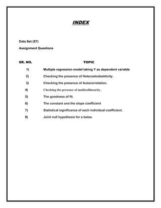
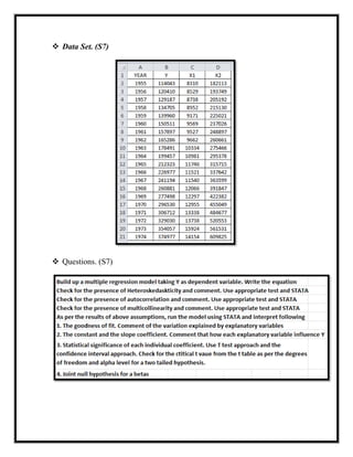
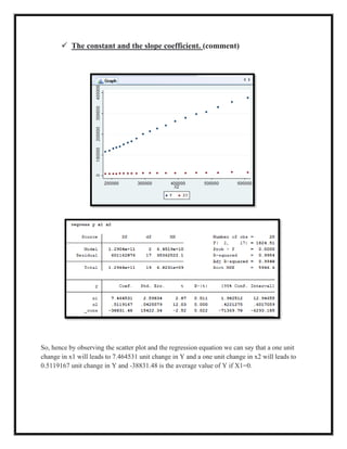
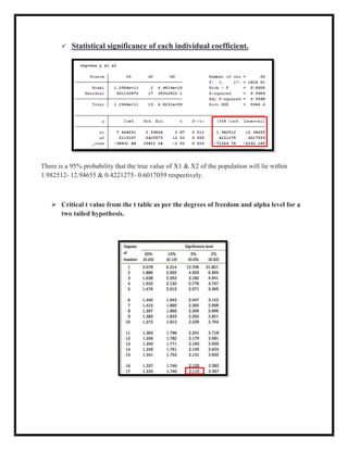
The document presents an applied econometric analysis utilizing a multiple regression model with various assessments, including heteroskedasticity, autocorrelation, and multicollinearity within the data set. The regression analysis indicates that y explains 99% of the variation from x1 and x2, with both predictors showing statistical significance. The presence of autocorrelation and multicollinearity is noted, leading to recommendations for robust standard errors and specific tests to address these issues.

1. ECO 8751: APPLIED ECONOMETRIC ANALYSIS I
SUBMISSION DATE: - 15th November,2020
SUBMITTED TO: -
Dr. Rajneesh Kler
Assistant professor
Economics & IB
School of management
GDGU
SUBMITTED BY: -
Rajat Sharma
190010301062
MBA Section- A
School of management
GDGU
SCHOOL OF MANAGEMENT, GDGU

2. INDEX
Data Set (S7)
Assignment Questions
SR. NO.
1)
2)
3)
4)
5)
6)
7)
8)
TOPIC
Multiple regression model taking Y as dependent variable
Checking the presence of Heteroskedaskticity.
Checking the presence of Autocorrelation.
Checking the presence of multicollinearity.
The goodness of fit.
The constant and the slope coefficient
Statistical significance of each individual coefficient.
Joint null hypothesis for a betas.

3. ❖ Data Set. (S7)
❖ Questions. (S7)

4. ✓ Multiple regression models taking Y as dependent variable.
➢ Multiple Regression Model Equation.
Ŷ= -38831.48+ 7.464531 (x1)+ 0.5119167 (x2)
➢ Interpretation.
One unit change in x1 will leads to 7.464531 unit change in Y and a one unit change in x2 will
leads to 0.5119167 unit change in Y and -38831.48 is the average value of Y if X1=0.

5. ✓ Checking the presence of Heteroskedaskticity.
Linear prediction Vs Residual scatter plot
X-Y scatter in the fitted values

6. Thus both the scatter plot mentioned above shows that there are little chances of the presence of
heteroskedasticity in the data set as the distribution of error is different at few X1.
➢ Comment on the presence of Heteroskedasticity.
Hence by, performing breush- pagan/ cook- Weisberg & Cameron and trivedi’s
decomposition of IM-test in stata it can be stated clearly that there is a little
presence of heteroskedasticity in the data set.
➢ Using robust standard error:

7. ✓ Checking the presence of Autocorrelation.
From the Durbin- Watson statistics table shown above, assuming 0.05 as a
significance level and given 20 & 3 as sample size & intercept it can be
interpret that the DL=0.77 & DU= 1.41.
OR

8. The value of the autocorrelation lies between the value 0.77 & 1.41.
By performing operation in stata, we came to know that the value of
d=0.6572771.
As the value of d<dl (0.6572771<0.77), it could be said that there is a
problem of autocorrelation exist in the data set.
➢ Use Newey corrected SE if autocorrelation is present:

9. ✓ Checking the presence of multicollinearity.
If there is 2 or more linear association between the independent variables then this can be named
as multicollinearity. As vif is more than 10 there are high chances that the multicollinearity may
present within a data set.
✓ The goodness of fit. (comment)
After performing a final regression analysis on stata it can be said that Y variable explains 99%
of the variation of the variable X1 & X2.

10. ✓ The constant and the slope coefficient. (comment)
So, hence by observing the scatter plot and the regression equation we can say that a one unit
change in x1 will leads to 7.464531 unit change in Y and a one unit change in x2 will leads to
0.5119167 unit change in Y and -38831.48 is the average value of Y if X1=0.

11. ✓ Statistical significance of each individual coefficient.
There is a 95% probability that the true value of X1 & X2 of the population will lie within
1.982512- 12.94655 & 0.4221275- 0.6017059 respectively.
➢ Critical t value from the t table as per the degrees of freedom and alpha level for a
two tailed hypothesis.

12. So to determine the t- value we will be dealing with the T- table where we will see the degree of
freedom as 17 which is number of observation – the inceptors (20-3=17), and assume the
significance level to be 5 % = 0.05.
And hence we will receive the T- value as 2.110.
✓ Joint null hypothesis for a betas.
Since the p- value of x1 & x2 is less than 0.05 that is (0.011<0.05) & (0.000<0.05) then we will
reject the null hypothesis.