Sunstone lectures

1. Lecture 5
Graphical Method
Operation
Research

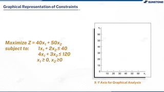
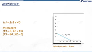
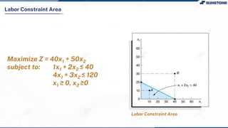
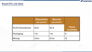
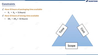
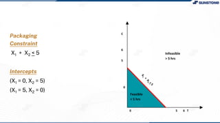
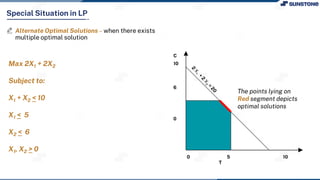
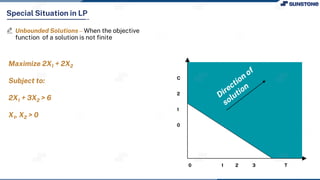
2. Objective
By the end of this class, we will be able to:
 Analyze Graphical Solution of Linear Programming
Models
 Recognize Graphical Representation of LP Models
 Explore Graphical Representation of Constraints
 Learn about Utilization of Feasible Solution Area
 Understand Corner Point Property
 Analyze Graphical Solutions
 Explore LP Characteristics

3. What is an Optimal Solution?

4.  Minimum or maximum value of an objective
function is the optimal solution
Optimal Solution

5. Now, question is…
How do we solve a linear programming problem?

6. There are different ways to solve these problems.
The problems having two variables can be solved
graphically.

7. Graphical solution is possible with two ‘decision variables’ (may be with three) in a linear programming
model
Graphical Solution - Linear Programming Models

9. Discussion
Decision Variables Objective Function
Constraints Non-negativity Restriction
Describe:

10. Graphical Representation - LP Models
Coordinates for
graphical
analysis 10
2
0
3
0
4
0
5
0
6
0
10 2
0
3
0
4
0
5
0
6
0
0

11. Graphical Representation of Constraints
X-Y Axis for Graphical Analysis
Maximize Z = 40x1 + 50x2
subject to: 1x1 + 2x2 ≤ 40
4x1 + 3x2 ≤ 120
x1 ≥ 0, x2 ≥0

12. Labor Constraint
1x1 + 2x2 ≤ 40
Intercepts
(X1 = 0, X2 = 20)
(X1 = 40, X2 = 0)
Labor Constraint - Graph

13. Labor Constraint Area
Labor Constraint Area
Maximize Z = 40x1 + 50x2
subject to: 1x1 + 2x2 ≤ 40
4x1 + 3x2 ≤ 120
x1 ≥ 0, x2 ≥0

14. Clay Constraint Area
Clay Constraint Area
4x1 + 3x2 ≤ 120
Intercepts
(X1 = 0, X2 = 40)
(X1 = 30, X2 = 0)

15. Graphical Representation of Constraints
Graphical Representation of Given
Constraints
Maximize Z = 40x1 + 50x2
subject to: 1x1 + 2x2 ≤ 40
4x1 + 3x2 ≤ 120
x1 ≥ 0, x2 ≥0

16. Feasible Solution Area
Feasible Solution Area
Maximize Z = 40x1 + 50x2
subject to: 1x1 + 2x2 ≤ 40
4x1 + 3x2 ≤ 120
x1 ≥ 0, x2 ≥0

17. Corner Point Property
The intersection points of two or more constraints that make up a feasible region are corner points.

18. Graphical Solution of Corner Point Method
Representation of Each Corner
Points
Maximize Z = 40x1 + 50x2
subject to constraints:
1x1 + 2x2 ≤ 40
4x1 + 3x2 ≤ 120
x1 ≥ 0, x2 ≥0

19. The Product Mix Problem Example
Decision to take:
Determine how
much to
manufacture for
more than 2
products
Objective is to:
Maximize profit
Constraints are:
Limited resources

20. Example: Dream Pvt. Ltd.
Two products:
Chocolate and
Biscuit
Decision:
Number of each
product to
manufacture per
month
Objective:
Maximize profit

21. Dream Pvt. Ltd. Data
Chocolates
(per packet)
Biscuits
(per packet)
Hours
Available
Profit Contribution Rs 6 Rs 5
Packaging 1 hr 1 hr 5
Mixing 3 hrs 2 hrs 12

22. Decision Variables:
X1 = No. of chocolates to
prepare
X2 = No. of biscuits to
prepare
Objective Function:
Maximize Z= 6X1 + 5X2

23. Constraints
Have 10 hours of packaging time available
• X1 + X2 < 5 (hours)
Have 12 hours of mixing time available
• 3X1 + 2X2 < 12 (hours)

24. Non-negativity
Negative number of chocolate or biscuit cannot be prepared
• X1 > 0
• X1 > 0

25. Model Summary
Maximize Z=6X1 + 5X2 (profit)
Subject to constraints are:
• X1 + X2 < 5 (packaging hrs)
• 3X1 + 2X2 < 12 (mixing hrs)
• X1 , X2 > 0 (non negativity)

26. Can you interpret this Pie Chart?

27. Graphical Solution
Graphical representation of LP Model provides insight into it and their solutions.
It is plotted in two dimension with X-Y axis and making points to plot the graph.

28. Packaging
Constraint
X1 + X2 < 5
Intercepts
(X1 = 0, X2 = 5)
(X1 = 5, X2 = 0)
0 5 6 T
C
6
5
0
Feasible
< 5 hrs
Infeasible
> 5 hrs

29. LP Characteristics
Feasible Region: The region formed by all
constraints including non-negative constraint
Corner Point Property: One or more corner
points must have an ‘optimal solution’
Optimal Solution: Where objective function
has an ideal (minimum or maximum) value

30. Mixing Line
3X1 + 2X2 < 12
Intercepts
(X1 = 0, X2 = 6)
(X1= 4, X2 = 0)
0 4 5 6 T
C
6
5
0
Feasible
< 5 hrs

31. Minimization Problem
Min Z=3 X1 + 2 X2
Constraints:
• 5 X1 + X2 > 10
• X1 + X2 > 6
• X1 + 4X2 > 12
• X1 , X2 > 0 (non negativity)

32. Mixed Constraints
Min Z=200 X1 + 400 X2
Constraints:
• X1 + X2 > 100
• X1 + 3X2 > 300
• X1 + 2X2 < 450
• X1 , X2 > 0 (non negativity)

33. Special Situation in Linear Programming

34. Redundant Constraints - In this the feasible region is not affected
Example: x < 10
x < 12
Special Situation in LP

35. Infeasibility – when there are no points to fulfill
the given constraints (lack of feasible region)
Example: x < 10
x < 15
Special Situation in LP

36. Alternate Optimal Solutions – when there exists
multiple optimal solution
Max 2X1 + 2X2
Subject to:
X1 + X2 < 10
X1 < 5
X2 < 6
X1, X2 > 0
0 5 10
T
C
10
6
0
The points lying on
Red segment depicts
optimal solutions
Special Situation in LP

37. Special Situation in LP
Unbounded Solutions – When the objective
function of a solution is not finite
Maximize 2X1 + 2X2
Subject to:
2X1 + 3X2 > 6
X1, X2 > 0
0 1 2 3 T
C
2
1
0

38. Activity
Maximize Z = 4x + 2y
Match the following
10X + 20Y ≤ 80
x1, x2.x3
X ≥ 0, Y ≥ 0
Non-negative Restriction
Objective Function
Decision Variable
Constraint

39. Maximize Z = 4x + 2y
Match the following
10X + 20Y ≤ 80
x1, x2.x3
X ≥ 0, Y ≥ 0
Non-negative Restriction
Objective Function
Decision Variable
Constraint
Activity