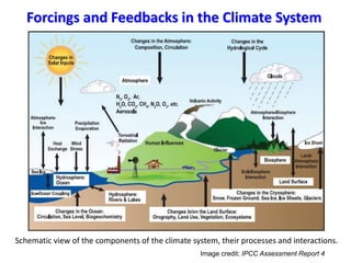
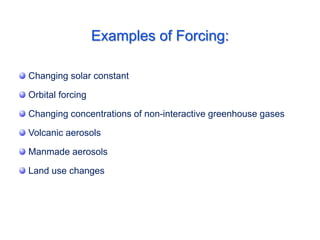
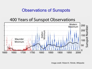
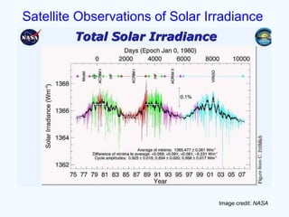
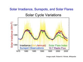
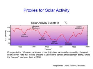
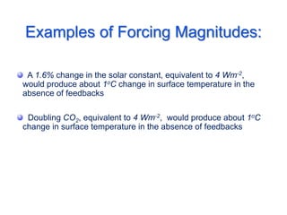
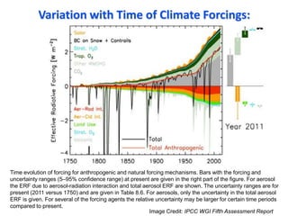
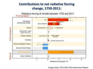
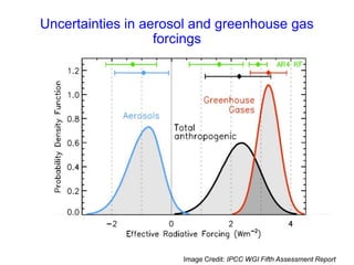
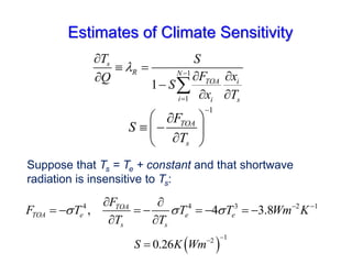
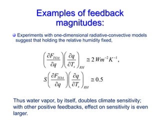
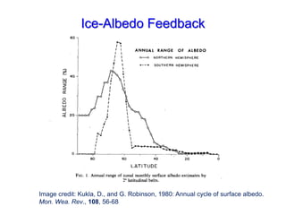
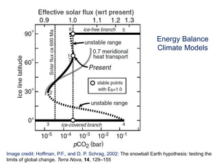
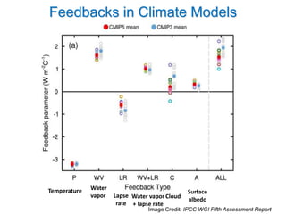
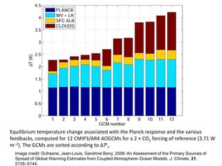
Climate Sensitivity, Forcings, And
Feedbacks
Forcings and Feedbacks in the Climate System
Schematic view of the components of the climate system, their processes and interactions.
Image credit: IPCC Assessment Report 4
Forcings and Feedbacks
Consider the total flux of radiation through the top of the
atmosphere:
TOA solar IR
F F F
 
The net top-of-the-atmosphere flux may be regarded as a
function of the surface temperature, Ts, and many other
variables xi :
 
1 2
, , ,.....
TOA TOA s N
F F T x x x

By the chain rule,
1
0
N
TOA TOA
TOA s i
i
s i
F F
F T x
T x
  

 
  
 

Now let’s call the Nth process a “forcing”,
1
1
1
1
0
N
TOA TOA
TOA s i
i
s i
N
TOA TOA i
s s
i
s i s
F F
F T x Q
T x
F F x
T T Q
T x T
   
  




 
   
 
  
  
  


Then
1
1
1
s
R N
TOA TOA i
i
s i s
T
F F x
Q
T x T
 


  
  


  

:
Q

1
1
1
s
R N
TOA i
i i s
T S
F x
Q
S
x T
 


 
 


 

1
TOA
s
F
Let S
T

 

 
 

 
Climate sensitivity
Climate sensitivity
without feedbacks
Feedback factors;
can be of either sign
Note that feedback factors do NOT add linearly
in their collective effects on climate sensitivity
Examples of Forcing:
Changing solar constant
Orbital forcing
Changing concentrations of non-interactive greenhouse gases
Volcanic aerosols
Manmade aerosols
Land use changes
Earth Rotation and Orbital Variations
Climate
Forcing by
Orbital
Variations
Milutin Milanković, 1879-1958
Portrait by Paja Jovanović (1859-1957)
Schematic of the Earth’s orbital changes
(Milankovitch cycles) that drive the ice age
cycles. ‘T’ denotes changes in the tilt (or
obliquity) of the Earth’s axis, ‘E’ denotes
changes in the eccentricity of the orbit (due to
variations in the minor axis of the ellipse), and
‘P’ denotes precession, that is, changes in the
direction of the axis tilt at a given point of the
orbit. Source: Rahmstorf and Schellnhuber
(2006): Der Klimawandel – Diagnose, Prognose,
Therapie, C. H. Beck, Munich
Climate Forcing and Response
Image credit: Robert A. Rohde, Wikipedia
Black: Time rate of change of ice volume
Red: Summer high latitude sunlight
Strong Correlation between High Latitude Summer Insolation
and Ice Volume
Huybers, P., Science 28 July 2006, Vol. 313 no. 5786 pp. 508-511, DOI:
10.1126/science.1125249
Solar Variability
Observations of Sunspots
Image credit: Robert A. Rohde, Wikipedia
Satellite Observations of Solar Irradiance
Image credit: NASA
Solar Irradiance, Sunspots, and Solar Flares
Image credit: Robert A. Rohde, Wikipedia
Proxies for Solar Activity
Image credit: Leland McInnes, Wikipedia
Changes in the 14C record, which are primarily (but not exclusively) caused by changes in
solar activity. Note that "before present" is used in the context of radiocarbon dating, where
the "present" has been fixed at 1950.
Image credit: William M. Connolley , Wikipedia
Inferences based on
observed relationships
between solar irradiance
and sunspot group
numbers (Wang et
al., 2005; Krivova et al.,
2010; Ball et al., 2012),
sunspot umbra and
penumbra and faculae
(Ball et al., 2012), or
cosmogenic isotopes
(Steinhilber et al., 2009;
Delaygue and Bard, 2011).
Image credit: IPCC WG1 Fifth Assessment Report
Reconstructions of Total Solar Irradiance
since1745,annual resolution series from Wang
et al. (2005) with and without an independent
change in the background level of irradiance,
Krivova et al. (2010) combined with Ball et
al. (2012), and 5-year time resolution series from
Steinhilber et al. (2009) and Delaygue and Bard
(2011).
Global average temperature, atmospheric CO2, and sunspot activity since 1850. Thick lines for
temperature and sunspots represent a 25 year moving average smoothing of the raw data.
Image credit: Leland McInnes, Wikipedia
Examples of Forcing Magnitudes:
A 1.6% change in the solar constant, equivalent to 4 Wm-2,
would produce about 1oC change in surface temperature in the
absence of feedbacks
Doubling CO2, equivalent to 4 Wm-2, would produce about 1oC
change in surface temperature in the absence of feedbacks
Greenhouse Gases
Carbon dioxide concentration in the atmosphere over the last
250 years based on both direct atmospheric measurements
and sampling of gases trapped in ice cores.
Image credit: Robert A. Rohde, Wikipedia
1750 1800 1850 1900 1950 2000
Image Credit: IPCC WGI Fifth Assessment Report
Variation in carbon
dioxide and
methane over the
past 20,000 years,
based on ice core
and other records
Image credit: IPCC Assessment Report 4
Carbon dioxide
Methane
Image credit: IPCC Assessment Report 4
Aerosols
Recent History of Volcanic Eruptions
Volcanic reconstructions of global mean aerosol optical depth (at 550 nm). Gao et al.
(2008) and Crowley and Unterman (2013) are from ice core data, and end in 2000 for
Gao et al. (2008) and 1996 for Crowley and Unterman (2013). Sato et al. (1993)
includes data from surface and satellite observations, and has been updated through
2011. Image Credit: IPCC WGI Fifth Assessment Report
Global sulfur dioxide emissions by (a) source and (b) end-use sector.
Emissions by source are the primary inventory result from this work.
Smith, S.J., and co-authors, 2011: Anthropogenic sulfur dioxide
emissions: 1850–2005. Atmos. Chem. Phys., 11, 1101–1116
Time evolution of RF due to aerosol-radiation interaction and BC on snow and ice. Multi-model results for
1850, 1930, 1980, and 2000 from ACCMIP for aerosol-radiation interaction (Shindell et al., 2013c) and
BC on snow and ice (Lee et al., 2013) are combined with higher temporal-resolution results from the
GISS-E2 and Oslo-CTM2 models (aerosol-radiation interaction) and Oslo-CTM2 (BC on snow and ice).
Uncertainty ranges (5–95%) for year 2010 are shown with vertical lines. Values next to the uncertainty
lines are for cases where uncertainties go beyond the scale. The total includes the RF due to aerosol-
radiation interaction for six aerosol components and RF due to BC on snow and ice.
Image Credit: IPCC WGI Fifth Assessment Report
SOA=secondary
organic aerosols
OC= Organic carbon
Variation with Time of Climate Forcings:
Image Credit: IPCC WGI Fifth Assessment Report
Time evolution of forcing for anthropogenic and natural forcing mechanisms. Bars with the forcing and
uncertainty ranges (5–95% confidence range) at present are given in the right part of the figure. For aerosol
the ERF due to aerosol-radiation interaction and total aerosol ERF are shown. The uncertainty ranges are for
present (2011 versus 1750) and are given in Table 8.6. For aerosols, only the uncertainty in the total aerosol
ERF is given. For several of the forcing agents the relative uncertainty may be larger for certain time periods
compared to present.
Contributions to net radiative forcing
change, 1750-2011:
Image Credit: IPCC WGI Fifth Assessment Report
Uncertainties in aerosol and greenhouse gas
forcings
Examples of Feedbacks:
Water vapor
Ice-albedo
Clouds
Biogeochemical feedbacks
Estimates of Climate Sensitivity
1
1
1
s
R N
TOA i
i i s
T S
F x
Q
S
x T
 


 
 


 

1
TOA
s
F
S
T

 

 
 

 
Suppose that Ts = Te + constant and that shortwave
radiation is insensitive to Ts:
4 4 3 2 1
, 4 3.8
TOA
TOA e e e
s s
F
F T T T Wm K
T T
    
 
       
 
 
1
2
0.26
S K Wm



Examples of feedback
magnitudes:
Experiments with one-dimensional radiative-convective models
suggest that holding the relative humidity fixed,
2 1
2 ,
0.5
TOA
s RH
TOA
s RH
F q
Wm K
q T
F q
S
q T
 
 
 
 

 
 
 
  
 
 
 

 
 
 
  
Thus water vapor, by itself, doubles climate sensitivity;
with other positive feedbacks, effect on sensitivity is even
larger.
Ice-Albedo Feedback
Image credit: Kukla, D., and G. Robinson, 1980: Annual cycle of surface albedo.
Mon. Wea. Rev., 108, 56-68
Energy Balance
Climate Models
Image credit: Hoffman, P.F., and D. P. Schrag, 2002: The snowball Earth hypothesis: testing the
limits of global change. Terra Nova, 14, 129–155
Feedbacks in Climate Models
Water
vapor Cloud
Surface
albedo
Lapse
rate
Water vapor
+ lapse rate
Temperature
Image Credit: IPCC WGI Fifth Assessment Report
Image credit: Dufresne, Jean-Louis, Sandrine Bony, 2008: An Assessment of the Primary Sources of
Spread of Global Warming Estimates from Coupled Atmosphere–Ocean Models. J. Climate, 21,
5135–5144.
Equilibrium temperature change associated with the Planck response and the various
feedbacks, computed for 12 CMIP3/AR4 AOGCMs for a 2 × CO2 forcing of reference (3.71 W
m−2). The GCMs are sorted according to ΔTe
s.

Climate Sensitivity, Forcings, And Feedbacks_2.pptx

  • 1.
  • 2.
    Forcings and Feedbacksin the Climate System Schematic view of the components of the climate system, their processes and interactions. Image credit: IPCC Assessment Report 4
  • 3.
    Forcings and Feedbacks Considerthe total flux of radiation through the top of the atmosphere: TOA solar IR F F F   The net top-of-the-atmosphere flux may be regarded as a function of the surface temperature, Ts, and many other variables xi :   1 2 , , ,..... TOA TOA s N F F T x x x  By the chain rule, 1 0 N TOA TOA TOA s i i s i F F F T x T x            
  • 4.
    Now let’s callthe Nth process a “forcing”, 1 1 1 1 0 N TOA TOA TOA s i i s i N TOA TOA i s s i s i s F F F T x Q T x F F x T T Q T x T                               Then 1 1 1 s R N TOA TOA i i s i s T F F x Q T x T                 : Q 
  • 5.
    1 1 1 s R N TOA i ii s T S F x Q S x T              1 TOA s F Let S T            Climate sensitivity Climate sensitivity without feedbacks Feedback factors; can be of either sign Note that feedback factors do NOT add linearly in their collective effects on climate sensitivity
  • 6.
    Examples of Forcing: Changingsolar constant Orbital forcing Changing concentrations of non-interactive greenhouse gases Volcanic aerosols Manmade aerosols Land use changes
  • 7.
    Earth Rotation andOrbital Variations
  • 8.
    Climate Forcing by Orbital Variations Milutin Milanković,1879-1958 Portrait by Paja Jovanović (1859-1957) Schematic of the Earth’s orbital changes (Milankovitch cycles) that drive the ice age cycles. ‘T’ denotes changes in the tilt (or obliquity) of the Earth’s axis, ‘E’ denotes changes in the eccentricity of the orbit (due to variations in the minor axis of the ellipse), and ‘P’ denotes precession, that is, changes in the direction of the axis tilt at a given point of the orbit. Source: Rahmstorf and Schellnhuber (2006): Der Klimawandel – Diagnose, Prognose, Therapie, C. H. Beck, Munich
  • 9.
    Climate Forcing andResponse Image credit: Robert A. Rohde, Wikipedia
  • 10.
    Black: Time rateof change of ice volume Red: Summer high latitude sunlight Strong Correlation between High Latitude Summer Insolation and Ice Volume Huybers, P., Science 28 July 2006, Vol. 313 no. 5786 pp. 508-511, DOI: 10.1126/science.1125249
  • 11.
  • 12.
    Observations of Sunspots Imagecredit: Robert A. Rohde, Wikipedia
  • 13.
    Satellite Observations ofSolar Irradiance Image credit: NASA
  • 14.
    Solar Irradiance, Sunspots,and Solar Flares Image credit: Robert A. Rohde, Wikipedia
  • 15.
    Proxies for SolarActivity Image credit: Leland McInnes, Wikipedia Changes in the 14C record, which are primarily (but not exclusively) caused by changes in solar activity. Note that "before present" is used in the context of radiocarbon dating, where the "present" has been fixed at 1950.
  • 16.
    Image credit: WilliamM. Connolley , Wikipedia
  • 17.
    Inferences based on observedrelationships between solar irradiance and sunspot group numbers (Wang et al., 2005; Krivova et al., 2010; Ball et al., 2012), sunspot umbra and penumbra and faculae (Ball et al., 2012), or cosmogenic isotopes (Steinhilber et al., 2009; Delaygue and Bard, 2011). Image credit: IPCC WG1 Fifth Assessment Report Reconstructions of Total Solar Irradiance since1745,annual resolution series from Wang et al. (2005) with and without an independent change in the background level of irradiance, Krivova et al. (2010) combined with Ball et al. (2012), and 5-year time resolution series from Steinhilber et al. (2009) and Delaygue and Bard (2011).
  • 18.
    Global average temperature,atmospheric CO2, and sunspot activity since 1850. Thick lines for temperature and sunspots represent a 25 year moving average smoothing of the raw data. Image credit: Leland McInnes, Wikipedia
  • 19.
    Examples of ForcingMagnitudes: A 1.6% change in the solar constant, equivalent to 4 Wm-2, would produce about 1oC change in surface temperature in the absence of feedbacks Doubling CO2, equivalent to 4 Wm-2, would produce about 1oC change in surface temperature in the absence of feedbacks
  • 20.
  • 21.
    Carbon dioxide concentrationin the atmosphere over the last 250 years based on both direct atmospheric measurements and sampling of gases trapped in ice cores. Image credit: Robert A. Rohde, Wikipedia 1750 1800 1850 1900 1950 2000
  • 22.
    Image Credit: IPCCWGI Fifth Assessment Report
  • 23.
    Image Credit: IPCCWGI Fifth Assessment Report
  • 24.
    Variation in carbon dioxideand methane over the past 20,000 years, based on ice core and other records Image credit: IPCC Assessment Report 4 Carbon dioxide Methane
  • 25.
    Image credit: IPCCAssessment Report 4
  • 26.
  • 27.
    Recent History ofVolcanic Eruptions Volcanic reconstructions of global mean aerosol optical depth (at 550 nm). Gao et al. (2008) and Crowley and Unterman (2013) are from ice core data, and end in 2000 for Gao et al. (2008) and 1996 for Crowley and Unterman (2013). Sato et al. (1993) includes data from surface and satellite observations, and has been updated through 2011. Image Credit: IPCC WGI Fifth Assessment Report
  • 28.
    Global sulfur dioxideemissions by (a) source and (b) end-use sector. Emissions by source are the primary inventory result from this work. Smith, S.J., and co-authors, 2011: Anthropogenic sulfur dioxide emissions: 1850–2005. Atmos. Chem. Phys., 11, 1101–1116
  • 29.
    Time evolution ofRF due to aerosol-radiation interaction and BC on snow and ice. Multi-model results for 1850, 1930, 1980, and 2000 from ACCMIP for aerosol-radiation interaction (Shindell et al., 2013c) and BC on snow and ice (Lee et al., 2013) are combined with higher temporal-resolution results from the GISS-E2 and Oslo-CTM2 models (aerosol-radiation interaction) and Oslo-CTM2 (BC on snow and ice). Uncertainty ranges (5–95%) for year 2010 are shown with vertical lines. Values next to the uncertainty lines are for cases where uncertainties go beyond the scale. The total includes the RF due to aerosol- radiation interaction for six aerosol components and RF due to BC on snow and ice. Image Credit: IPCC WGI Fifth Assessment Report SOA=secondary organic aerosols OC= Organic carbon
  • 30.
    Variation with Timeof Climate Forcings: Image Credit: IPCC WGI Fifth Assessment Report Time evolution of forcing for anthropogenic and natural forcing mechanisms. Bars with the forcing and uncertainty ranges (5–95% confidence range) at present are given in the right part of the figure. For aerosol the ERF due to aerosol-radiation interaction and total aerosol ERF are shown. The uncertainty ranges are for present (2011 versus 1750) and are given in Table 8.6. For aerosols, only the uncertainty in the total aerosol ERF is given. For several of the forcing agents the relative uncertainty may be larger for certain time periods compared to present.
  • 31.
    Contributions to netradiative forcing change, 1750-2011: Image Credit: IPCC WGI Fifth Assessment Report
  • 32.
    Image Credit: IPCCWGI Fifth Assessment Report Uncertainties in aerosol and greenhouse gas forcings
  • 33.
    Examples of Feedbacks: Watervapor Ice-albedo Clouds Biogeochemical feedbacks
  • 34.
    Estimates of ClimateSensitivity 1 1 1 s R N TOA i i i s T S F x Q S x T              1 TOA s F S T            Suppose that Ts = Te + constant and that shortwave radiation is insensitive to Ts: 4 4 3 2 1 , 4 3.8 TOA TOA e e e s s F F T T T Wm K T T                    1 2 0.26 S K Wm   
  • 35.
    Examples of feedback magnitudes: Experimentswith one-dimensional radiative-convective models suggest that holding the relative humidity fixed, 2 1 2 , 0.5 TOA s RH TOA s RH F q Wm K q T F q S q T                                   Thus water vapor, by itself, doubles climate sensitivity; with other positive feedbacks, effect on sensitivity is even larger.
  • 36.
    Ice-Albedo Feedback Image credit:Kukla, D., and G. Robinson, 1980: Annual cycle of surface albedo. Mon. Wea. Rev., 108, 56-68
  • 37.
    Energy Balance Climate Models Imagecredit: Hoffman, P.F., and D. P. Schrag, 2002: The snowball Earth hypothesis: testing the limits of global change. Terra Nova, 14, 129–155
  • 38.
    Feedbacks in ClimateModels Water vapor Cloud Surface albedo Lapse rate Water vapor + lapse rate Temperature Image Credit: IPCC WGI Fifth Assessment Report
  • 39.
    Image credit: Dufresne,Jean-Louis, Sandrine Bony, 2008: An Assessment of the Primary Sources of Spread of Global Warming Estimates from Coupled Atmosphere–Ocean Models. J. Climate, 21, 5135–5144. Equilibrium temperature change associated with the Planck response and the various feedbacks, computed for 12 CMIP3/AR4 AOGCMs for a 2 × CO2 forcing of reference (3.71 W m−2). The GCMs are sorted according to ΔTe s.